Doppler synchronization of pulsating phases by time delay

Abstract

Synchronization by exchange of pulses is a widespread phenomenon, observed in flashing fireflies, applauding audiences and the neuronal network of the brain. Hitherto the focus has been on integrate-and-fire oscillators. Here we consider entirely analytic time evolution. Oscillators exchange narrow but finite pulses. For any non-zero time lag between the oscillators complete synchronization occurs for any number of oscillators arranged in interaction networks whose adjacency matrix fulfils some simple conditions. The time to synchronization decreases with increasing time lag.

I Introdution

The emergence of coherent structures in time and space though synchronization occurs across the entire breadth of science: vibrating atoms, firing neurons, flashing fireflies, clapping audiences etc. and has therefore been studied intensively from a mathematical viewpoint Strogatz (2004); Pikovsky et al. (2001); Néda et al. (2000a).

Synchronization is often analyzed in models which explicitly favor phase synchronization, e.g. in the seminal Kuramoto model Kuramoto (1975); Pikovsky et al. (2001) and in diffusively coupled models (see e.g. Nishikawa and Motter (2010); Pereira (2011)). In these schemes the net-interaction between oscillators indeed vanishes in the synchronized state.

However, in many cases, such as fireflies Winfree (2001); Lewis and Cratsley (2008); Trimmer et al. (2001), cardiac cells, neuronal system and applauding audiences Néda et al. (2000a, b) the interaction between oscillators consists in the exchange of brief pulses, which persist even when the system fully synchronize. Since Mirollo and Strogatz’s influential 1990 paper Mirollo and Strogatz (1990) such systems are often described by a set of non-analytically evolving integrate-and-fire oscillators. Each oscillator is described by a load variable, which is taken to have a concave dependence on a monotonously increasing phase. When the load reaches a certain threshold, relaxation occurs instantaneously and a pulse is send to all connected oscillators. Receiving oscillators jump discontinuously forward by a given amount. For such systems Mirollo and Strogatz showed Mirollo and Strogatz (1990) that full synchronization always occurs. Later Ernst, Pawelzik and Geisel Ernst et al. (1995) demonstrated that for excitatory-only couplings, synchronization depends on phase lag, whereas the presence of inhibitory couplings leads to full in-phase synchronization.

The treatment of pulse oscillators in terms of non-analytic integrate-and-fire oscillators is more a tradition than a necessity. In the present paper we assume that each oscillator is represented by a phase $\theta_{i}(t)$ whose time $t$ derivative is always equal to a constant rate plus a sum of smooth but narrow pulses emitted by surrounding oscillators coupled with strength $J$. Synchronization (asymptotically vanishing phase difference) always occurs for this system if pulses arrive with a non-zero time lag $\delta t\,$ for a very wide class of adjacencies, including the mean-field setting often considered in the literature.

Given the previous results for pulse oscillators Mirollo and Strogatz (1990); Ernst et al. (1995) and to illuminate the more detailed discussion below it is natural to begin our analysis of two pulse exchanging phases by considering Dirac’s delta pulses for the interaction.

$$\dot{\theta}_{1}(t) = \omega+J\sum_{n\in{\mathbb{Z}}}\delta(\theta_{2}(t-\delta t)-n))$$

$$\dot{\theta}_{2}(t) = \omega+J\sum_{n\in{\mathbb{Z}}}\delta(\theta_{1}(t-\delta t)-n))$$ (1)

Integrating the time derivatives tells us that $\theta_{1}$ “jumps” each time $\theta_{2}$ passes through an integer value, $\theta_{1}(t)\mapsto\theta_{1}(t)+J$, and vise versa for $\theta_{2}$. Let $\theta_{1}(0)>\theta_{2}(0)$, it is straight forward to see, Fig. 1, that the two phases are unable to synchronize though in the case of a finite time delay they may leapfrog each other, as the jump of one oscillator can make the other skip its.

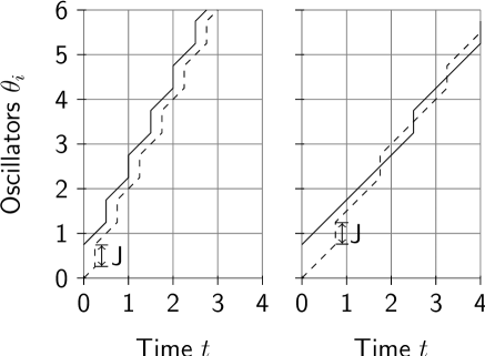
Figure 1: The time evolution of two oscilators (solid and dashed lines) exchanging pulses according to Eq. 1. Left panel: $\delta t=0$, right panel: $\delta t=0.5$.

Obviously Dirac delta pulses are unrealistic. Pulses emitted by real systems will have a finite width and a smooth time dependence (Eq. (2) below). The introduction of smooth pulses changes the behavior in an essential way. As will be explained below synchronization now takes place whenever a time lag is present, $\delta t>0$, and in this case complete synchronization occurs for all smooth pulses.

General model – We now consider $n$ coupled oscillators, each described by a single degree of freedom $\theta_{i}$, with $i=1,2,\dots,n$, and each with the same eigenfrequency $\omega$:

$$\dot{\theta}_{i}(t)=\omega+\sum_{j}J_{ij}\sigma(\theta_{j}(t-\delta t\,))$$ (2)

Oscillators are coupled through an adjancency matrix $J_{ij}$ and a feedback function $\sigma(\theta)$ which has period $\xi$. It is only through $\sigma(\theta)$ that periodicity is implemented: $\sigma(\theta_{i})$ describes the effect that the state of $\theta_{i}$ (say, the flashing of a firefly) has on any other oscillator. As opposed to other models often studied in synchronization, such as the Kuramoto model Pikovsky et al. (2001), the effect of $\sigma$ does not disappear in the synchronized state.

We chose $\dot{\theta}_{i}>0$ at all times such that $\theta_{i}(t)$ are monotonically increasing functions in time. This is achieved by choosing $\sigma(\theta)>0$. In our numerical study below we use a comb of normalised Gaussians with period $\xi$ and width $w$, $\sigma(\theta)=\sum_{n=-\infty}^{\infty}\mathchoice{e^{-(x+n\xi)^{2}/(2w^{2})}}{\operatorname{exp}\left(-(x+n\xi)^{2}/(2w^{2})\right)}{\operatorname{exp}\left(-(x+n\xi)^{2}/(2w^{2})\right)}{\operatorname{exp}\left(-(x+n\xi)^{2}/(2w^{2})\right)}(2\pi w^{2})^{-1/2}=\xi^{-1}\vartheta_{3}(\pi x/\xi,\mathchoice{e^{-2w^{2}\pi^{2}/\xi^{2})}}{\operatorname{exp}\left(-2w^{2}\pi^{2}/\xi^{2})\right)}{\operatorname{exp}\left(-2w^{2}\pi^{2}/\xi^{2})\right)}{\operatorname{exp}\left(-2w^{2}\pi^{2}/\xi^{2})\right)}$, the Jacobi theta function.

In natural systems time delay is inevitable. We show that $\delta t\,>0$ is crucial for synchronization. We use this term in a strong sense: For any pair $i,j$ of oscillators $\lim_{t\to\infty}\theta_{i}(t)-\theta_{j}(t)=\mu_{ij}\xi$ with $\mu_{ij}\in\mathds{Z}$, i.e. the phase difference between any two oscillators converges to an integer multiple of the period of $\sigma$, which implies $\lim_{t\to\infty}\dot{\theta}_{i}-\dot{\theta}_{j}=0$. By inspection it is clear that for the synchronized state to exist indefinitely, $\sum_{j}J_{ij}=\tilde{J}$ needs to be independent of $i$, which means that if synchronization takes place, the difference between any $\theta_{i}(t)$ and the solution $\tilde{\theta}(t)$ of

$$\dot{\tilde{\theta}}(t)=\omega+\tilde{J}\sigma(\tilde{\theta}(t-\delta t\,))$$ (3)

with appropriate initial conditions vanishes asymptotically. Provided $\tilde{J}\neq 0$, the eigenfrequency $\omega$ can be absorbed into $\sigma$, using $\sigma(\theta)\to\sigma(\theta)+\omega/\tilde{J}$.

Simple two oscillator case – We now demonstrate that under very general conditions the system in Eq. Eq. (2) will synchronize in the long time limit. First we consider the simple case of two oscillators, i.e. $n=2$ and $J_{ij}=1-\delta_{ij}$. By considering $\dot{\theta}_{1}/\dot{\theta}_{2}$, it is easy to show that $\theta_{1}(t)-\theta_{2}(t)$ is periodic if $\delta t\,=0$, i.e. synchronization in the strong sense above does not occur without time delay, rather, entrainment is inevitable. However, integrating the equation of motion Eq. (2) numerically on the basis of a simple Euler method suggests differently. Better numerical schemes, such as the Runge Kutta Press et al. (1992) method, remove the spurious synchronization, which depends on the integration time step and therefore hints at the rôle of the time delay effectively implemented by the forward derivative used in the most naïve Euler scheme.

We now analyze in detail the effect of a time delay by considering Eq. (2) with $\delta t\,>0$. A linear stability analysis for small $\delta t\,$ and small deviations $\theta_{i}(t)-\tilde{\theta}(t)$ reveals that any positive $\delta t\,$ leads to a synchronized state.We present the calculation briefly in the following for $n=2$ and $J_{ij}=1-\delta_{ij}$.

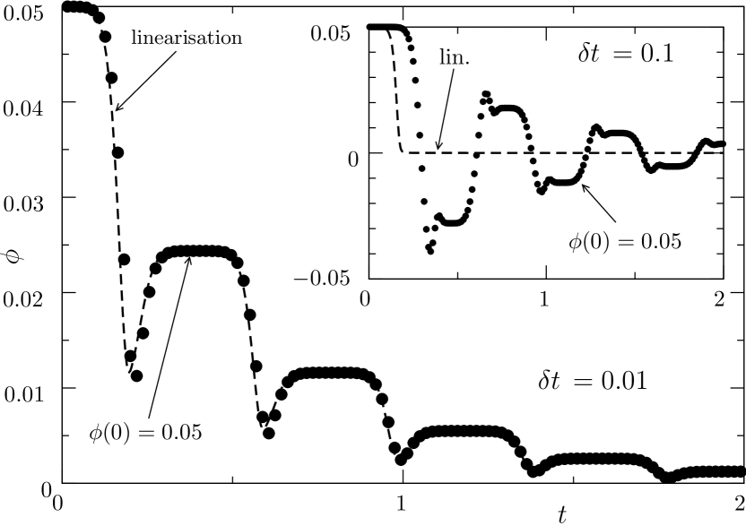
Figure 2: Comparison of $\phi(t)=(\theta_{1}(t)-\theta_{2}(t))/2$ from a numerical integration of Eq. (2) (filled circles) and the linear approximation (dashed line) Eq. (5), with $\phi(t)=0.05$ and $\delta t\,=0.01$. Parameters are $n=2$, $J_{ij}=1-\delta_{ij}$, $\omega=2$, $\xi=1.01$ and $w=0.1$, so that $\psi\approx 0.3934$. The inset compares of full solution and linear approximation for $\phi(0)=0.05$ and $\delta t\,=0.1$.

The equations of motion of $\phi(t)=\mathchoice{\frac{1}{2}}{(1/2)}{\frac{1}{2}}{(1/2)}(\theta_{1}(t)-\theta_{2}(t))$ and $\bar{\theta}=\mathchoice{\frac{1}{2}}{(1/2)}{\frac{1}{2}}{(1/2)}(\theta_{1}(t)+\theta_{2}(t))$ are

$$\dot{\phi}(t) = \mathchoice{\frac{1}{2}}{(1/2)}{\frac{1}{2}}{(1/2)}(\sigma(\theta_{2}(t-\delta t\,))-\sigma(\theta_{1}(t-\delta t\,)))$$ (4a)

$$\dot{\bar{\theta}}(t) = \mathchoice{\frac{1}{2}}{(1/2)}{\frac{1}{2}}{(1/2)}(\sigma(\theta_{2}(t-\delta t\,))+\sigma(\theta_{1}(t-\delta t\,)))+\omega$$ (4b)

which we study to first order in $\phi$ and $\delta t\,$ and find (for details see Pruessner et al. )

$$\phi(t)=\phi(0)\frac{\dot{\bar{\theta}}(0)}{\dot{\bar{\theta}}(t)}\operatorname{exp}\left(-2\delta t\,\tilde{J}^{2}\int_{\bar{\theta}(0)}^{\bar{\theta}(t)}\textrm{d}\theta\frac{\sigma^{\prime 2}(\theta)}{\omega+\tilde{J}\sigma(\theta)}\right)$$ (5)

with $t(\bar{\theta})=\int_{\bar{\theta}(0)}^{\bar{\theta}}\textrm{d}\theta(\omega+\sigma(\theta))^{-1}$. As the integrand is strictly positive, synchronization takes place in this approximation for all $\delta t\,>0$. Fig. 2 shows that the linearized solution is a very good approximation of the full system Eq. (2).

The characteristic time to synchronization is estimated in the following way. Define

$$\psi = \int_{0}^{\xi}\textrm{d}\bar{\theta}\frac{1}{\omega+\tilde{J}\sigma(\bar{\theta})}\approx\int_{0}^{\xi}\frac{\textrm{d}\bar{\theta}}{\dot{\bar{\theta}}}$$ (6a)

$$S = \int_{0}^{\xi}\textrm{d}\bar{\theta}\frac{\sigma^{\prime 2}(\bar{\theta})}{\omega+\tilde{J}\sigma(\bar{\theta})}$$ (6b)

where $\psi$, to leading order, is the time for $\sigma(\bar{\theta}(t))$ to go through one period, i.e. $\bar{\theta}(t+\psi)\approx\bar{\theta}(t)+\xi$. $S$ corresponds to the integral in the exponent of Eq. (5) for $\bar{\theta}(t)=\bar{\theta}(0)+\xi$. As the integrand is periodic we estimate

$$\int_{\bar{\theta}(0)}^{\bar{\theta}(t)}\textrm{d}\theta\frac{\sigma^{\prime 2}(\theta)}{\omega+\tilde{J}\sigma(\theta)}\approx\frac{t}{\psi}S$$ (7)

and rewrite Eq. (5) $\phi(t)=\phi(0)(\dot{\bar{\theta}}(0)/\dot{\bar{\theta}}(t))\mathchoice{e^{-t/\tau}}{\operatorname{exp}\left(-t/\tau\right)}{\operatorname{exp}\left(-t/\tau\right)}{\operatorname{exp}\left(-t/\tau\right)}$, with the characteristic synchronization time

$$\tau\simeq\frac{\psi}{2\tilde{J}^{2}\delta t\,S}\ ,$$ (8)

inversely proportional to the time delay $\delta t\,$.

Network of oscillators – The above picture can be extended to arbitrary coupling matrices $J_{ij}$, or a (weighted) network adjacency matrix. The only constraint is $\sum_{j}J_{ij}=\tilde{J}$ independent from $i$, similar to a Markov matrix. Motivated by the observation that the two parameters used above, $\bar{\theta}$ and $\phi$, are based on the eigenvectors of the matrix $J_{ij}=1-\delta_{ij}$ studied for $n=2$, we consider the time evolution of $\left\langle i|\phi(t)\right\rangle$, i.e. of “normal modes”, where $\left\langle i\right|$ is the $i$th left eigenvector of $J$, which, we assume for simplicity, has $n$ linearly independent eigenvectors. For simplicity, we normalize $\left\langle i|j\right\rangle=\delta_{ij}$. The matrix $J$ is not necessarily symmetric so generally $\left(\left\langle i\right|\right)^{\dagger}\neq\left|i\right\rangle$. Due to the Markov property, there is a pair of left and right eigenvectors with eigenvalue $\tilde{J}$, which in the following is denoted by $\left\langle 1\right|$ and $\left|1\right\rangle=\sum_{i}^{n}\left|e_{i}\right\rangle$ respectively, where $\left|e_{i}\right\rangle$ denotes the canonical basis of the $\mathds{R}^{n}$.

The state of the entire system is written in vector form as $\left|\theta(t)\right\rangle=\sum_{i}^{n}\left|e_{i}\right\rangle\theta_{i}(t)$. The column vector $\left|\phi(t)\right\rangle$ is the deviation $\left|\phi(t)\right\rangle=\left|\theta(t)\right\rangle-\bar{\theta}(t)\left|1\right\rangle$ of $\left|\theta(t)\right\rangle$ from $\bar{\theta}(t)=\left\langle 1|\theta(t)\right\rangle$ anticipating that $\bar{\theta}(t)$ represents the asymptotically synchronised state. Following the procedure above, one finds

$$\left\langle i|\phi(t)\right\rangle=A_{i}\left(\frac{T(\bar{\theta}(t))}{T_{0}}\right)^{\frac{\lambda_{i}}{\tilde{J}}}\\ \times\operatorname{exp}\left(\lambda_{i}(\tilde{J}-\lambda_{i})\delta t\int_{\bar{\theta}(0)}^{\bar{\theta}(t)}\frac{\sigma^{\prime 2}(\theta^{\prime})}{T(\theta^{\prime})}\textrm{d}{\theta^{\prime}}\right)$$ (9)

where $T_{0}=T(\bar{\theta}(0))$ and $T(\bar{\theta})=\omega+\tilde{J}\left(\sigma(\bar{\theta})-\delta t\,\dot{\bar{\theta}}(\bar{\theta})\sigma^{\prime}(\bar{\theta})\right)=\dot{\bar{\theta}}(\bar{\theta})+\mathcal{O}(\delta t\,^{2})$.

The amplitudes $A_{i}$ are determined by the initial projections $\left\langle i|\phi(0)\right\rangle=A_{i}$. Eq. (9) also applies to $i=1$, yet $\left\langle 1|\phi(t)\right\rangle=0$ by construction so that $A_{1}=0$. The special case $\tilde{J}=0$ (so that $\dot{\bar{\theta}}=\omega$ to linear order) coincides with the limit $\tilde{J}\to 0$, where

$$\lim_{\tilde{J}\to 0}\left(\frac{T(\bar{\theta}(t))}{T_{0}}\right)^{\frac{\lambda_{i}}{\tilde{J}}}=\mathchoice{e^{\lambda_{i}\sigma(\bar{\theta})/\omega-\delta t\,\lambda_{i}\sigma^{\prime}(\bar{\theta})}}{\operatorname{exp}\left(\lambda_{i}\sigma(\bar{\theta})/\omega-\delta t\,\lambda_{i}\sigma^{\prime}(\bar{\theta})\right)}{\operatorname{exp}\left(\lambda_{i}\sigma(\bar{\theta})/\omega-\delta t\,\lambda_{i}\sigma^{\prime}(\bar{\theta})\right)}{\operatorname{exp}\left(\lambda_{i}\sigma(\bar{\theta})/\omega-\delta t\,\lambda_{i}\sigma^{\prime}(\bar{\theta})\right)}$$ (10)

to leading order, assuming $T_{0}=\omega$ for simplicity.

Since $T(\bar{\theta})$ is periodic, the long-term behaviour of $\left\langle i|\phi(t)\right\rangle$ depends crucially on the sign of the real part of $\lambda_{i}(\tilde{J}-\lambda_{i})$. If it is negative, the projection has an approximate synchronization time

$$\tau_{i}=\frac{\int_{0}^{\xi}\textrm{d}{\bar{\theta}}\frac{1}{\omega+\tilde{J}\sigma(\bar{\theta})}}{-\mathchoice{\Re\left(\lambda_{i}(\tilde{J}-\lambda_{i})\right)}{\Re(\lambda_{i}(\tilde{J}-\lambda_{i}))}{\Re(\lambda_{i}(\tilde{J}-\lambda_{i}))}{\Re(\lambda_{i}(\tilde{J}-\lambda_{i}))}\delta t\,\int_{0}^{\xi}\textrm{d}\bar{\theta}\frac{\sigma^{\prime 2}(\bar{\theta})}{\omega+\tilde{J}\sigma(\bar{\theta})}}\ ,$$ (11)

corresponding to Eq. (8). Here $\mathchoice{\Re\left(\cdot\right)}{\Re(\cdot)}{\Re(\cdot)}{\Re(\cdot)}$ denotes the real part. The usual mean-field setup $J_{ij}=a(1-\delta_{ij})$ has one eigenvalue $\tilde{J}=(n-1)a$ and $n-1$ eigenvalues $\lambda_{i}=-a$, so that $\lambda_{i}(\tilde{J}-\lambda_{i})=-na^{2}$ has a negative real part provided $a^{2}$ has a positive one, i.e. in particular for all real $a$. The mean-field theory thus always synchronises, as does the special case of a lattice Laplacian.

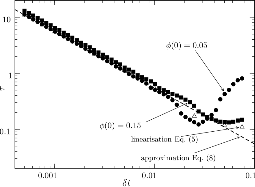
Figure 3: Plot of the synchronization time estimated from the window averaged phase difference $\theta_{1}(t)-\theta_{2}(t)$ (average taken over a time period $t^{*}$ so that $\bar{\theta}(t)=\bar{\theta}(t-t^{*})-\xi$). The filled symbols refer to results based on Eq. (2), the empty triangles to Eq. (5) and the line to Eq. (8). Parameters as in Fig. 2.

The perturbative result Eq. (9) can be compared to the numerical integration of the system. We used a fourth order Runge-Kutta integration scheme Press et al. (1992); Pruessner et al. and show in Fig. 3 that the derived synchronization time compares very well (for time delays up to 5% to 10% of the synchronized period) to that of the linearised result, Eq. (5) and to the estimate Eq. (8).

Mechanism – How is synchronization achieved? Fig. 4 shows $\sigma(\theta_{i}(t))$ and $\dot{\theta_{i}}(t)$ as a function of $t$ for $n=2$. Synchronization occurs because $\theta_{2}$ experiences a greater increase in speed by $\sigma(\theta_{1}(t-\delta t\,))$ than $\theta_{1}$ does by $\sigma(\theta_{2}(t-\delta t\,))$. This asymmetry comes about because $\theta_{2}$ is relatively fast itself when $\sigma(\theta_{2}(t))$ goes through its maximum and $\theta_{1}$ is relatively slow when $\sigma(\theta_{1}(t))$ goes through its maximum. As a result the maximum $\sigma(\theta_{1}(t))$ is broadened as a function of time, and $\sigma(\theta_{2}(t))$ is narrowed (this effect is minute and thus not visible in Fig. 4). Therefore, the maximum of $\sigma(\theta_{1}(t-\delta))$ enters into $\dot{\theta_{2}}$ for a longer time period than $\sigma(\theta_{2}(t-\delta))$ enters into $\dot{\theta_{1}}$, leading to a speedup of $\theta_{2}$ relative to $\theta_{1}$. In summary, synchronization is result of oscillator $i$ being slow or fast when going through the maximum of the function $\sigma(\theta_{i})$. What rôle has the time delay in this? The time delay ensures that the trailing oscillator $\theta_{2}$ receives a boost at a time when $\sigma(\theta_{2}(t))$ goes through a maximum, while the leading $\theta_{1}$ receives its boost at a time when $\sigma(\theta_{1}(t))$ goes through a local minimum. Without the time delay, the effect of the speed-up and the slowdown would indeed be perfectly symmetric.

We notice that the mechanism underlying the synchronization supported by Eq. (2) is a kind of Doppler effect that makes the received pulse change its duration when the sending oscillator changes its speed.

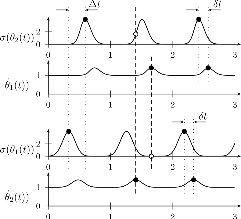
Figure 4: We see that $\theta_{1}$ is ahead of $\theta_{2}$, with the maximum of $\sigma(\theta_{2}(t))$ displaced by $\Delta t$ (as indicated) to the right relative to that of $\sigma(\theta_{1}(t))$, as initialised. At a given time, $\theta_{2}$ still has to pass through the maximum of $\sigma(\theta_{2}(t))$ when $\theta_{1}$ already has. The phase speed $\dot{\theta}_{1,2}(t)$ is essentially $\sigma(\theta_{2,1}(t))$ shifted by $\delta t\,$ to the right, as indicated by the dotted lines. As a result, the maximum of $\dot{\theta}_{2}$ nearly aligns with the maximum of $\sigma(\theta_{2}(t))$, i.e. $\theta_{2}$ is fast when $\sigma(\theta_{2}(t))$ goes through the maximum (dashed line), thereby narrowing it. In turn, $\theta_{1}$ passes very quickly through a low value of $\sigma(\theta_{1}(t))$, relatively broadening in turn the maximum of $\sigma(\theta_{1}(t))$.

Equation Eq. (2) provides a remarkably simple mechanism for synchronization. Because oscillators lagging behind by a certain amount catch up in every period of $\sigma(\bar{\theta})$ by an amount of phase difference proportional to the phase difference at the beginning of the period, the model can immediately be extended to one with different eigenfrequencies $\omega_{i}$ of oscillators or some variation in $\sum_{j}J_{ij}$ with $i$ or of $\sigma$ and even $\delta t\,$. An analysis of such extensions follows the derivation above, see Pruessner et al. . It will generally lead to entrainment.

Synchronisation by time delay is a viable explanation for natural synchronisation phenomena whenever oscilators respond to the duration of the pulse received. Fireflies are known to be able to change the pulse duration and female fireflies are sensitive to that Lewis and Cratsley (2008). The exact way a clapping audience reaches synchrony Néda et al. (2000a, b) can be analyzed sufficiently accurately to establish whether people change the duration of the individual clap Peltola et al. (2007) in the process of reaching synchrony.

References

- Strogatz (2004) S. Strogatz, Sync: The emerging science of spontaneous order. (Penguin, London, England, 2004), 2nd ed.
- Pikovsky et al. (2001) A. Pikovsky, M. Rosenblum, and J. Kurths, Synchronization. A universal concept in nonlinear sciences (Cambridge University Press, Cambridge, UK, 2001), 1st ed.
- Néda et al. (2000a) Z. Néda, E. Ravasz, Y. Brechet, T. Vicsek, and A.-L. Barabási, Nature 403, 849 (2000a).
- Kuramoto (1975) Y. Kuramoto, in International Symposium on Mathematical Problems in Theoretical Physics, edited by H. Araki (Springer-Verlag, Berlin, Germany, 1975), vol. 39 of Lecture notes in physics, pp. 420–422.
- Nishikawa and Motter (2010) T. Nishikawa and A. Motter, Proc. Natl. Acad. Sci. USA 107, 10342 (2010).
- Pereira (2011) T. Pereira (2011), eprint arXiv:1112.2297v1.
- Winfree (2001) A. Winfree, The geometry of biological time (Spriger, 2001), 2nd ed.
- Lewis and Cratsley (2008) S. M. Lewis and C. K. Cratsley, Annu. Rev. Entomol. 53, 293 (2008).
- Trimmer et al. (2001) B. A. Trimmer, J. R. Aprille, D. M. Dudzinski, C. J. Lagace, S. M. Lewis, T. Michel, S. Qazi, and R. M. Zayas, Science 292, 2486 (2001).
- Néda et al. (2000b) Z. Néda, E. Ravasz, T. Vicsek, Y. Brechet, and A.-L. Barabási, Phys. Rev. E 61, 6987 (2000b).
- Mirollo and Strogatz (1990) R. Mirollo and S. Strogatz, SIAM J. Appl. Math. 50, 1645 (1990).
- Ernst et al. (1995) U. Ernst, K. Pawelzik, and T. Geisel, Phys. Rev. Lett. 74, 1570 (1995).
- Press et al. (1992) W. H. Press, S. A. Teukolsky, W. T. Vetterling, and B. P. Flannery, Numerical Recipes in C (Cambridge University Press, New York, NY, USA, 1992), 2nd ed.
- (14) G. Pruessner, S. Cheang, and H. J. Jensen, in preparation.
- Peltola et al. (2007) L. Peltola, C. Erkut, P. R. Cook, and V. Valimaki, IEEE Audio, Speech, Language Process. 15, 1021 (2007), ISSN 1558-7916.