Mixture Models of Endhost Network Traffic

Abstract

In this work we focus on modeling a little studied type of traffic, namely the network traffic generated from endhosts. We introduce a parsimonious parametric model of the marginal distribution for connection arrivals. We employ mixture models based on a convex combination of component distributions with both heavy and light-tails. These models can be fitted with high accuracy using maximum likelihood techniques. Our methodology assumes that the underlying user data can be fitted to one of many modeling options, and we apply Bayesian model selection criteria as a rigorous way to choose the preferred combination of components. Our experiments show that a simple Pareto-exponential mixture model is preferred for a wide range of users, over both simpler and more complex alternatives. This model has the desirable property of modeling the entire distribution, effectively segmenting the traffic into the heavy-tailed as well as the non-heavy-tailed components. We illustrate that this technique has the flexibility to capture the wide diversity of user behaviors.

I Introduction

In the last decade or so there has been a tremendous amount of research done in the area of Internet traffic modeling (e.g., [26, 6, 19] to name a few). Traffic models are helpful in solving a wide range of problems, including traffic engineering, service provisioning, routing, and network performance evaluation. To date, however, the vast majority of traffic modeling research has focused on traffic seen inside a network: at routers, gateways, or servers. Relatively little work has been done to model traffic as seen at endhosts, such as laptops or desktops.

The paucity of endhost traffic models is limiting, because many problems can benefit from an understanding of the nature of endhost traffic. Recently there is increased interest in modeling and describing the behavior of enterprise end users [13, 29]. IT management is driving this trend, as it faces an increasingly heterogeneous computing environment. Autonomic computing is heading towards self-diagnosis for fault identification, and endhost profiles are being explored for security purposes [3] and resource management. For example, in [17] the authors design mechanisms to allow hosts to participate in network management, traffic engineering and other operational decisions by explicitly controlling host traffic. To better calibrate such applications, a deep understanding of end user traffic is needed.

The most likely reason that endhost traffic models are so scarce is that it is difficult to obtain the raw measurements needed, since those measurements require the express consent of each user in a sufficiently large set. Furthermore, such measurements essentially require installing a collection tool directly on each user’s machine — a tool whose management requires considerable goodwill from the affected users.

The value of endhost models combined with the difficulty of endhost instrumentation have motivated some efforts that have tried to infer endhost traffic properties from an observation point inside the network [14, 29]. While such approaches have shed some light, they are fundamentally limited — for example, when users are mobile. What is needed for a comprehensive view of endhost traffic is a measurement tool that moves with the user and continues to observe network traffic as the user switches between different networks and different environments (e.g., work and home).

In this work we deploy such a tool and analyze its outputs to develop models for end user traffic. We study a population of 270 enterprise users over a period of five weeks (§III). Our tool collects all packet headers entering and exiting the machine, on all networking interfaces. To accomplish this, we solicited enterprise employees to sign up on a voluntary basis for the trace collection. Participants explicitly gave consent for data collection; each user downloaded and installed the data collection software on their personal machines.

Starting with this rich dataset, we focus on careful modeling of user activity, in particular the arrival process of flow initiations. A main focus of our work is developing a robust method for distributional modeling of flow arrivals. To that end, we go beyond simple parameter estimation and attack the model selection problem.

In our approach we overcome concerns about the use of goodness-of-fit testing for choosing probability models, and in particular for power law models, about estimating their scaling parameter. Commonly used methods for estimating the scaling parameter include the Hill estimator and least-squares regression on a log-log plot of the histogram. The Hill estimator is notoriously tricky since it relies on estimating a cut-off below which the central part of the distribution is disregarded, to concentrate on just the scaling parameter of the small subset of data in the tail [23, 20], while extracting the scaling parameter by performing a least-squares regression has been shown to little more than a misleading heuristic, of questionable statistical value. In [5], the authors highlight the lack of care pervasive in the literature on power laws, and apply a rigorous approach to applying goodness of fit methods. In the process they review numerous power law claims that have been made, and find that claims of power law tails among well-known supposedly-“power law” datasets are not supported by the data. In our work, we demonstrate an efficient estimator that uses the entire data set (rather than just the tail).

Hence, our first contribution is in modeling endhost traffic using mixture models (§IV-A) to estimate model parameters. A mixture model is a convex combination of component distributions, where the parameters of the component distributions as well as the mixture parameter are estimated from data.

To discriminate among the class of mixture models we need a criterion, the commonly applied one being goodness-of-fit. The limitation of this approach is that goodness-of-fit tests, and their associated $P$-values, are meant to rule out hypotheses (i.e. to reject the hypothesis). This is certainly useful for steering data collection, but they do not provide an acceptance criterion. The best one can hope for with this method, in a statistical sense, is to say that a given model has not been ruled out by the data. In our situation, with effectively an endless stream of data as a source, in the limit of large data, the probability of any model decreases along with goodness of fit’s $P$-values, and the result is that any reasonable model will be rejected. What is needed to confirm the proper choice of model is not model fitting but rather model selection, a different problem with a different statistical basis.

Model selection methods give us a quantitative criterion that lets us explore a wider class of models than has hitherto been considered. Thus we do not presuppose a single parametric distribution model; instead we start with a class of nested mixture models (i.e. a family of models where one is a subset of another) and use Bayes Factors [18] to select the best model in the class for a user’s data. For the large sample sizes that we consider, the log Bayes Factor can be well approximated by the difference of two models’ Bayesian Information Criteria (BIC). Since it is a requirement for Bayes Factors comparisons to compare both models on the full sample data (not just the distributional tail), as a side benefit we produce complete models as they vary over the set of users.

Our second contribution is thus to validate an approach that makes available a richer, non-parametric (in the sense of the number of parameters is not fixed before model selection) class of models for traffic modeling. We use Maximum Likelihood methods (§IV-B) for parameter estimation and validate (§V) the accuracy of our parameter estimation technique on synthetic data created from mixture models. Our success with this method in modeling endhost traffic suggests that it might be fruitful to explore using this modeling technique to other heavy-tailed datasets of network measurements.

Our third contribution lies in the results of extensive application of this method on our endhost traffic data (§VI). We observe that the distribution of flow arrival counts can be generally characterized as monotonically declining, from a mode at zero. Hence we can eliminate a vast majority of possible component distributions (such as, e.g., Gaussian or Poisson) and concentrate on mixtures of various exponential and Pareto distributions. Since mixtures of exponentials in particular constitute a very flexible framework, restricting to these two distributions does not severely limit our modeling ability. Thus our model selection process considers various combinations of the Pareto (P) component with one or more exponential (E) distribution components to form a nested family of mixture models. This family includes mixtures such as EP, EEP, and P.

We find that for the metrics we study (flow arrivals and idle period lengths), the vast majority of users are well modeled by the EP distribution; a much smaller number are better modeled by P and EEP models. Here the flexibility of our approach is a strength, because our method does not insist that all users need to be described by the same model.

Our final contribution lies in examining the results of our modeling. We expose and highlight strong invariants across users (§VI), but also illustrate the nature of the diversity among different users. For example, we demonstrate that tail properties and mixing fractions differ dramatically across our set of users. Finally in §VII we look into which applications and services contribute traffic to the exponential and pareto components of our models.

II Related Work

Heavy tailed statistics have been documented in numerous phenomena in network traffic; in the popularity of web pages [4], in traffic demands [11]; in network topology [20], in TCP inter-arrival times  [10], in wireless LAN traffic [21], and many others. As mentioned earlier, most of this work analyzes traffic collected from inside the network at locations where anywhere from hundreds to millions of users’ traffic is aggregated. To the best of our knowledge, our work is the first to study connection traffic generated directly on user laptops.

The seminal work by Leland et al. [19] studied LAN traffic and convincingly demonstrated that actual network traffic is self-similar or long-range dependent in nature (i.e., bursty over a wide range of time scales). Our work differs in two ways. First, that study’s Ethernet LAN data captured the aggregated traffic of many users, whereas we focus on models for individual user traffic. Second, we observe the power law nature of traffic in the first-order statistics of traffic rates, rather than in the second-order autocorrelation properties. Both approaches result in estimating a power-law parameter, but the meaning of the parameters should not be confused.

Work closer to our study is reported in [8, 1]. Those studies captured HTTP requests through instrumentation in web browsers or proxies, and so are similar to ours in focusing on a traffic seen at a fixed set of endhosts. Results from those studies were used in developing tools for generating representative user-level HTTP traffic [2]. However, those studies did not look at the total set of an individual endhost’s pattern of connections over time. This crucial difference makes our results more useful for general traffic modeling. In fact, as we shall see, the aggregate traffic on endhosts is influenced strongly by applications other than the Web. An important aspect of this distinction is that our data also includes network traffic that is machine generated (i.e. not user generated). Machine generated traffic comes from background enterprise applications, chatty protocols, and the many auto-update checking mechanisms (e.g., for software and firewall rule updates) that are typically installed on corporate laptops.

Another end user study looks at data from Neti@Home users, and models think time as well as bytes sent and received for TCP and UDP connections [28]. They do not model traffic at the granularity of connection arrivals. In [3], the authors report on the diversity in distributional tails of user behaviors. This diversity is captured by a simple metric, the 99^th percentile of various distributions on user protocol traffic. The models proposed in our paper capture user tail diversity with richer measures, such as the slope parameter $\alpha$ of the Pareto distribution from the EP model.

The idea of using mixture models for Internet traffic has been proposed in other contexts before [12]. That work proposes using hyperexponential models to approximate heavy-tailed distributions. Thus it is not about explicitly modeling data collected from the Internet, but more about fundamental methods for approximations of heavy-tailed distributions. The advantage of their work is that their effort provides analytically tractable representations that can be used subsequently for queueing theory models. However, the disadvantage (as the authors acknowledge) is that their mixture models have a large number of parameters. In our work, we obtain parsimonious models with a small number of parameters. All of our models range from having 1 to at most 5 parameters; most users are well modeled using only 3 parameters. Further, in constrast to the fitting-oriented approach [12], our work does not assume the presence of a heavy-tailed component ahead of time. It is entirely possible for our mixture model to assign a negligible Pareto component to a dataset.

III Dataset Description

The dataset used in this paper consists of traces collected at 270 enterprise end-hosts (90% laptops), spanning a period of approximately 5 weeks. Each end-host was associated with a unique user for the entire trace collection period, and ran a corporate standard build of Windows XP which included a number of enterprise IT applications.

Packet-level traces were collected on the end-hosts, rather than at a network tap, providing a longitudinal view of the traffic even as the end-hosts moved in and out of the network and switched between interfaces (wired and wireless). The trace logging software included a wrapper around WinDump to log packet headers and a homegrown application which sampled user-activity indicators (# keystrokes, # mouse clicks) and CPU load every second. The trace logging software tracked changes in IP address and network interface, and restarted the traffic trace collection at such times. The logged data was uploaded opportunistically a few times a day to a central server (the logging was paused during the upload). The trace collection effort yielded approximately 400 Gb of packet header traces. The packet traces were converted to flows (in the standard five-tuple sense) using BRO [25].

The starting time of each flow generates a point process in continuous time that we bin over non-overlapping constant duration time-windows to create a time series for each user. Each user trace was binned for 8 different window sizes, starting at 4 seconds, and increasing in multiples of 2, up to 512 seconds. Each bin contains a count of the new flow arrivals. The flow count events within each time-window or bin are the random variables modeled in this work. In our datasets the median sample size was 9771 intervals, and the maximum was 264,000. Zeros could occur in bins because the host was turned off (or asleep), or else if the host was disconnected from the network during that bin. We filter out all such bins and in the resulting data, we see zeros only because there were no flows originated in that bin (and the machine was turned on). That being said, we mainly focus on modeling the flow events when the counts are nonzero since our goal is to characterize the flow traffic when the network is being used.

IV Methodology

IV-A Mixture Models with Heavy Tails

A mixture model is a likelihood function composed of a convex combination of probability densities. Such models are familiar in the Statistics literature, [9][15] and have become a mainstay in the machine learning community  [16]. A mixture model can be thought of as a hierarchical model where the mixing weights determine the probability of each of the component models, which in turn generate the sample points. Since all components share the same support, any sample point could in principle have been generated by any component, but possibly with vanishingly small probability.

A mixture model is defined by a probability density. For component densities, $f_{i}(x)$, and mixture fractions $m_{i}$, the finite mixture model of $k$ components, with parameters $\mathbf{m},\mathbf{\theta}$ is the convex combination given by:

$$f(x\,|\,\mathbf{m},\theta)=\sum^{k}_{i=1}{m_{i}}f_{i}(x\,|\,\theta_{i}),$$ (1)

$${\hbox{s.t. }}\sum^{k}_{i=1}m_{i}=1,m_{i}>0.$$

where the $\theta$ are the component parameters, and $\mathbf{m}=m_{1}\ldots m_{k}$. The degrees of freedom of the model is the count of parameters, e.g. for $k$ components, each with a single parameter, the full model will have $k+(k-1)$ parameters.

We consider the following nested family of models: a Pareto only model labeled (P), a mixture of one exponential and one Pareto (EP), and a mixture of two exponentials and one Pareto (EEP). The “pure power-law” model we fit is

$$f(x\,|\,\alpha)=Cx^{-\alpha}=\frac{1}{\zeta(\alpha,x_{min})}x^{-\alpha},x\in{\cal N}$$ (P)

where $x$ takes on positive integer values, for which we use the discrete version of the Pareto density (referred to also as the Zeta) in our models. The value of the Zeta function in the normalizing constant for the discrete Pareto is

$$\zeta(\alpha,x_{min})=\sum^{\infty}_{n=0}(n+x_{min})^{-\alpha}.$$ (2)

The exponential - Pareto model is defined as

$$f(x\,|\,\mathbf{m},\lambda_{1},\alpha)=m_{1}\lambda_{1}{e^{-\lambda_{1}{x}}}$$ (EP)

$${}+(1-m_{1})Cx^{-\alpha}.$$

The mixture variable adds another degree of freedom, revealing the relative contribution of the components.

The two exponential - Pareto mixture density model is:

$$f(x\,|\,\mathbf{m},\lambda_{1},\lambda_{2},\alpha)=m_{1}\lambda_{1}{e^{-\lambda_{1}{x}}}$$ (EEP)

$${}+m_{2}\lambda_{2}{e^{-\lambda_{2}{x}}}$$

$${}+(1-m_{1}-m_{2})Cx^{-\alpha}.$$

We were motivated originally to consider these models because visual exploration of the data showed a traffic flow distributions with mode left-most, then a monotone decrease with a linear segment on a semi-log plot in the dense part of the distribution, followed by a long, heavy tail.

The intent behind using a family of models is to capture the diversity of each user’s machine. In principle, any combination of the 3 component distributions could be discovered, although in practice we always see a heavy-tailed component. In terms of degrees of freedom, these are very parsimonious models; the EP model has 3 parameters, and the EEP has only 5.

IV-B Estimating Model Parameters

The model parameters are estimated using maximum likelihood. The maximum likelihood estimate (MLE) has numerous attractive qualities. If the model contains the true data generating distribution, and is differentiable in quadratic mean (DQM) [30], the MLE converges to the true parameters at a rate $O(1/\sqrt{n})$. Pareto distributions and mixtures of DQM models satisfy differentiability in quadratic mean. Even if the model does not contain the true data generating distribution, the MLE converges to the best approximation to the true distribution within the model’s constraints at a rate $O(1/\sqrt{n})$. The MLE is also asymptotically efficient, so no other estimator can obtain a better asymptotic variance than the MLE.

Instead of a conventional Expectation-Maximization (EM) methods, we solved the MLE as constrained optimization problem using an interior point method [31] to enforce the constraints on the model parameters. We found EM converged slowly, probably due to the similar shapes of the components. Interior point methods are iterative optimization methods that enforce constraints by adding a weighted concave barrier function that steeply decreases to $-\infty$ at the boundary of the constraint set, preventing the estimates from violating constraints. The weight on the barrier is decreased while using the previous solution for initialization, and a new solution is computed. The weight continues to be reduced until the barrier becomes negligible. A typical choice of barrier function is $\log$. Thus, for the EP model with log likelihood function $l$, the constrained optimization problem

$$\max_{\begin{subarray}{c}m_{1}+m_{2}=1\,m_{1},m_{2}>0\\ \alpha>1,\,\lambda>0\end{subarray}}l(m_{1},m_{2},\alpha,\lambda;x)$$

may be solved by the sequence of unconstrained problems

$$\max_{m_{1},\alpha,\lambda} \qquad l(m_{1},1-m_{1},\alpha,\lambda;x)+c_{1}^{(t)}\log(\alpha-1)$$

$$+c_{2}^{(t)}\log(\lambda)+c_{3}^{(t)}\log(1-m_{1})+c_{3}^{(t)}\log(m_{1})$$

where $m_{2}$ has been replaced by $1-m_{1}$ and the weights on the barrier $c_{i}^{(t)}\to 0^{+}$ as $t\to\infty$. By convention, we take $log(x)=-\infty$ if $x\leq 0$. These unconstrained problems can be solved using the optim() function in the statistical programming language R, which implements a Quasi-Newton optimization method. To exclude obviously bad solutions, we also added constraints $\alpha<4$ and $\lambda<3.5$ so that the Pareto and the exponential parameters did not grow not too large.

Since the mixture model typically contains local optima, we performed the optimization multiple times with random initializations to find the global maximum. We also used small initial values of $c_{i}=0.01$ for the regularization parameters and reduced them to $c_{i}=10^{-8}$ in 3 steps to prevent the initial unconstrained problem and regularization path from unduly influencing the search for the global maximum.

IV-C Model Selection

Given two probability models for the same sample, model selection is a means of comparing which model is more probable. Our explanation of model selection, borrows extensively from Kass and Raftery [18], and is based upon the numerical value of the comparative metric called a Bayes Factor ($BF$), . Following Jefferies, to quote, “The Bayes Factor is a summary of the evidence in favor on one scientific theory, represented by a statistical model, as opposed to another.” This can be understood using the odds ratio form of Bayes rule, where the posterior odds—the ratios of posteriors—between two models, is expressed as the product of the $BF$ and the prior odds. So, for example to compare the model $\mathcal{M}_{P}$ to the proposed model $\mathcal{M}_{EP}$, the posterior odds will be

$$\frac{\mathsf{P}(\mathcal{M}_{EP}\,|\,\mathcal{D})}{\mathsf{P}(\mathcal{M}_{P}\,|\,\mathcal{D})}=\frac{\mathsf{P}(\mathcal{D}\,|\,\mathcal{M}_{EP})}{\mathsf{P}(\mathcal{D}\,|\,\mathcal{M}_{P})}\frac{\mathsf{P}(\mathcal{M}_{EP})}{\mathsf{P}(\mathcal{M}_{P})}$$ (3)

where the middle term in this equation, the Bayes factor, $BF$, is defined as the ratio of marginal likelihoods:

$$BF_{EP,P}=\frac{\mathsf{P}(\mathcal{D}\,|\,\mathcal{M}_{EP})}{\mathsf{P}(\mathcal{D}\,|\,\mathcal{M}_{P})}$$ (4)

The larger $BF$, the greater the weight of evidence for the EP model.

This criterion is similar to a maximum likelihood ratio, but rather than taking the probability at the maximum, one integrates over the range of parameters $\mathbf{\theta}$, resulting in a correction for the degrees of freedom of the models. Adding more parameters to a model and thus increasing its degrees of freedom can only increase the likelihood at the maximum but does not necessarily improve marginal likelihood. This criterion trades off simplicity with accuracy—a built-in “Occam’s Razor.”

IV-D Interpreting The Weight of Evidence

Interpreting the magnitude of a $BF$ is commonly done by considering the ratio as an odds ratio, e.g., odds of 20 to 1 in favor of the model in the numerator corresponds to a $BF=20$, or, using natural logs, $\log BF\simeq 3$. Of course, the test is symmetric and the ratio may go either way. A negative $\log BF_{EP,P}$ is evidence against the EP model, in favor of P. We give precedence to the conventional model, and hence require an log odds-ratio significantly greater than zero—we use 10—to chose EP. If the EP model is selected, then we compute $\log BF_{EEP,EP}$. Again, if this factor is above 10, then EEP is selected, otherwise the final choice is EP.

Table I shows a standard convention[18] that we adopt for interpreting the strength of Bayes Factors with their suggested labels. Our threshold of 10 is well into the “decisive” range, corresponding to an odds ration of greater than 20,000.

TABLE I: Interpretation of Bayes Factor strengths

Odds	$\log_{10}(BF)$	$\log(BF)$	Strength of comparison
20:1	1.3	3	“substantial”
100:1	2	4.5	“strong”
1000:1	3	7	“decisive”

IV-E Approximation by BIC

In practice the integral implied by $\mathsf{P}(\mathcal{M}\,|\,\mathcal{D},\mathbf{\theta})$ that requires a prior over the $\mathbf{\theta}$ is rarely done explicitly. Experiments on our large sample data showed that likelihood values are infinitesimal and strongly peaked around their maximum at $\mathbf{\hat{\theta}}$. Not surprisingly numerical integration works poorly, so a common recourse is to approximate the integral by the Laplace approximation. The Laplace approximation can be further approximated by the Bayes Information Criterion (BIC). BIC is often presented as a correction to maximum log likelihood to account for the degrees of freedom of a model. The BIC is defined as

$$\mbox{BIC}=\log\mathsf{P}(\mathcal{D}\,|\,\mathcal{M},\mathbf{\hat{\theta}})-\log(N)\cdot d/2$$ (5)

where $N$ is the sample size and $d$ is the numbers of parameters in the model. In our experimental work we computed both Laplace approximations and BIC corrections and found to our satisfaction that they agreed with each other to within a fraction of a percent on the data used.

With the BIC approximation, the log Bayes Factor becomes

$$\log BF_{EP,P}=\mbox{BIC}_{EP}-\mbox{BIC}_{P}$$ (6)

The BIC criterion is appealing as a standard procedure in that it can be applied even when the priors on $\mathbf{\theta}$ are hard to choose.

V Validation

We validated our model-fitting and selection method in two ways, first to show that the estimates produced are accurate, and secondly that the selection mechanism we propose can distinguish among any of the three models. To do this we use synthetic data where the true value of the parameters of the generating data is known. The test data consisted of pseudo-random samples with known parameters $\hat{\alpha},\hat{m_{\{1,2\}}},\hat{\lambda_{\{1,2\}}}$, generated from each of the three models in the family P, EP and EEP. Since the test data is generated according to the same probability law to which the data is being fit, the models do not have to approximate the sample; we know that the data is in the same class as one of the three models. The same can be said of the Pareto-tail fitting procedure used, that is, by ignoring the dense part of the distribution contributed by the “E” component, will see a pure power-law sample.

V-A Estimation Accuracy

The tail-fitting method used for comparison is a widely used (e.g., [24]) tool [7] for estimating the $\alpha$ parameter of $\alpha$-stable distributions, based on a scaling property of sums of heavy-tailed random variables. An attractive property of this estimator is that it is nonparametric and easy to apply. Characteristic of Hill-estimator based methods [27] the method also estimates where the tail begins by computing a minimum value with which to select a range of the sample. We used a publicly available implementation, called aest.

Fig. 1 compares the EP mixture model estimates of $\alpha$ on EP sample data over eight test values of $\alpha$ as indicated along the top of the plot. For each test value, we ran 100 test cases of 10000 samples each, with $m_{1}=0.5$ and $\lambda$ values chosen from the interval $[0.1..0.3]$. The box-and-whiskers plots show the distributions of the 100 estimated $\alpha$ values by the two different methods, as compared to the true values shown by the dotted horizontal line.

The $\hat{\alpha}$ values box-and-whiskers obtained via the aest test are paired with the MLE plots on the same data in each panel of the figure. We see that the range of $\hat{\alpha}$’s in the columns subtitled “ML” for the mixture model estimates, is almost always within a few percent of the true value. Interestingly we see that the aest $\hat{\alpha}$’s have a higher variance and tend to be biased. In some sense, this is not surprising as the authors published results [7] acknowledge similar estimate variances when the underlying distribution is Pareto. Similarly the bias may well be due to the exponential component bleeding into the tail estimate, due to the method using a larger range of the sample, at the expense of less purity. The aest estimator has several fundamental limitations. The Hill estimator only uses the tail portion of the data, whereas the MLE mixture model uses all the data. Hence, it throws away information and cannot achieve the same efficiency as the MLE. This validates that our MLE optimization algorithm for the EP mixture model converges to an accurate value when run on simulated EP data.

Figure 1: When tested on synthetic Pareto-tailed data over $1<\alpha\leq 2$ an EP mixture model estimator performs significantly better than the well-known AEST method.

V-B Correct Model Selection

Next we confirm that model selection by pair-wise comparison of BIC scores does indeed select the right model, despite the model set consisting of nested models. Since the EEP model subsumes the other two, the model with more parameters will always fit better, so the correct choice is driven by the penalty dues to the BIC parameter count term.

We ran 100 test cases over a range of sample sizes from 500 to 20,000 points, in the style of an empirical “design of experiments” to find what sample sizes were necessary to show adequate model selection results. We ran 3 pair-wise comparisons: EP vs. P on EP data, EEP vs EP on EP data and EEP vs EP on EEP data. In a fourth comparison, EP vs. P on P data, the informal results were so strong that it didn’t merit a formal run.

In Table 2, we summarize the ability of our model selection method to distinguish the 3 hypotheses. For each test, we state the number of samples and the Bayes Factor level so achieved, using the conventions substantial, strong, or decisive in Table  I. For the first two tests we list sample sizes for two levels.

The more complicated the model comparison, the larger the sample required for the same strength of differentiation. In short, the EP model can be selected “substantially” with around traces of no less than 1000 samples. The EEP model requires about 10 times the sample to be selected at the same level. This is reason to believe that requiring samples on the order of a few thousand (or at most 10,000) is a fairly light requirement for this class of models in our domain.

In practice, the next section reveals that the actual Bayes Factors computed on the data have values ranging in the hundreds, with sample sizes in the thousands and tens of thousands—clearly at the “decisive” level, and orders of magnitude larger than seen in these validation tests! Also, the $m_{i}$ mixture fractions mimic the model selection rules closely. This is to be expected, since $m_{i}$ represents the probability of the component $i$ in the sample. When its estimated value approaches zero, it is equivalent to selecting a model lacking that component. Were it not for the cost in sample size and computation one could always just estimate the most inclusive model and select the final model by eliminating components whose mixing fractions approach zero.

Truth	Model Choice:	Min Number	$log_{10}$ BF
		Samples	strength
EP	EP vs. P	1000	substantial
		5000	decisive
EP	EEP vs. EP	1000	substantial
		10,000	strong
EEP	EEP vs. EP	9000	substantial

TABLE II: Sample sizes and the strength of comparison they achieve with simulated data, for different model comparisons.

VI Results

We now use our methodology to select the best model for each of our 270 users. We make some observations about our users based on the selected models and model parameters.

VI-A Choice of Models

Figure 2: Boxplot of BIC comparison for Pareto vs. 2-component Mixture Model.

Figure 3: Comparison of EP and EEP models

In Fig. 2 we plot the log of the Bayes Factor (or difference in BICs) of the P and EP models. The x-axis labels indicate the bin size that was used when the models were computed. For each bin size, we computed the $\log BF_{EP,P}$ for each user. For each bin size, we use box plots to show the distribution of the Bayes factors over all the users. We can see that for nearly all users we can select the two component EP model as ‘decisive’, according to Table 2. There are a very small number of users whose whose $\log BF_{EP,P}$ was near zero. Recall that when two models are considered indistinguishable, the model with fewer parameters is selected. The methodology selects a Pareto-only model for roughly a dozen of our endhost machines. Not only is the two component mixture model EP preferred for all the other users, but it is strongly preferred as evidenced by the high Bayes factor values. We observe a small trend here in that as the bin sizes increase, the log Bayes factor ratio gets larger. This empirical observation indicates that for larger bin sizes, the exponential component plays an increasingly dominant role. Although not shown here on graphs, we also observed that as the bin sizes increase, the median mixing fraction $m$ increases. This corroborates the observation that the exponential plays an increasing role for larger bin sizes.

Next we compare the EP and EEP models. Fig. 3 plots the distribution (as a boxplot) of the Bayes factors over all users, for each of 4 bin sizes. Interestingly, we see that at bin sizes of 64 and 128, the Bayes factors are close to zero for the majority of the users. Since the two models are fairly indistinguishable here, we again select the model of lower complexity, namely EP for nearly all the users. (There are a few outliers that would elect EEP). At larger bin sizes, we do see some users for whom the EEP model is selected. Overall, our method assigns the EEP model to roughly 30% of the users and the EP model to the remaining 70%.

Fig. 4 shows which model is selected by the methodology for all of our endhost machines. Overall we see that only a handful of users are given the Pareto-only model, and between 15%-40% of user machines are best modeled by EEP (depending upon the bin size). Overall, the EP model is selected for 50-85% of the users, again depending upon the bin size. We conclude two things from this section. First, the flexibility we have built into our methodology is important and needed because the best model for one endhost is not necessarily the same for another endhost. Second, for the majority of the endhosts, the mixture model consisting of one exponential and one Pareto is clearly the preferred model.

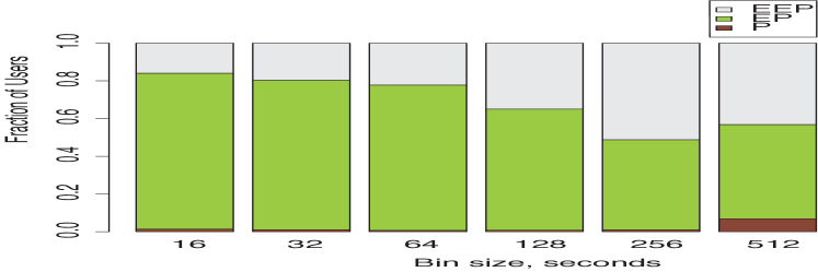
Figure 4: Choice of models based on Bayes Factors for different users. Each bar represents the same users with a different binning time window

VI-B User Behavior

As indicated in §II, there is a growing interest in understanding the range of variation of user behavior. We now look at some model details to explore the range of parameters selected across users, and the amount of mixing between the two model components. We computed an EP model for all our users, and examined the resulting $\alpha$ and $\lambda$ values.

We first observed that there is little correlation between $\alpha$ and $\lambda$ values within each EP model. This is reassuring, as it indicates that the fitting process does not introduce dependencies between the two component distributions, and that properties of one distribution do not affect the other.

In Fig. 5 we show the histograms of $\alpha$ values over users for a bin size of 64 sec. We see that the values of $\alpha$ range from 1.3 to 2.3 across the users; different users have very different properties in terms of the heaviness of the tail of the distrbution. Roughly 1/6 of our users have $\alpha<1.5$ implying a fairly heavy tail, while most users have $\alpha$ values around 1.6 or 1.7. It is interesting that we do have a small number users (4) with $\alpha>2$ indicating a finite second moment.

Figure 5: Histogram of estimated $\alpha$ values across users.

We now look more closely at how the users mix the two components of the model. A value of $m$ close to 0 implies that the model is dominated by the exponential distribution, (when $m=0$ there is no Pareto component in the model). Similarly when $m$ is close to 1 the Pareto component dominates the behavior of the model ($m=1$ indicates there is no exponential component). The $m$ parameter is considered a soft model selection factor because of its ability to indicate the strength of each component of the distribution. The MLE estimates determine $m$ from the data, which is why it can be viewed as a soft model selection factor. To see the range of $m$ values chosen across our users, we provide a histogram of this mixing factor in Fig. 6. The frequency on the y-axis denotes the number of users whose $m$ parameter is that indicated on the x-axis. Only 3 users picked an $m$ very close to 1, indicating that the pure Pareto model suites practically none of our users—in agreement with the Bayes Factors conclusions. Most of the users have an $m$ parameter less than 0.4, and roughly half of our users had $m<0.25$ indicating the dominance of the exponential component in the model. The $m$ values are fairly well spread across the range 0 to 0.5 (roughly). We can also interpret this range of $m$ as a indication of user diversity, in that their mixing fractions differ substantially.

Figure 6: Histogram of estimated $m_{\alpha}$ across users.

VII Traffic Composition

The traffic models described are high level models that are agnostic as to the particular kinds of applications or services present in the traffic. There are several interesting questions that can be asked about the underlying generative processes that underlie the traffic. Are there particular applications and ports that tend to occur more often in the exponential component of the distribution, or the pareto component? Are there particular types of traffic that are generated by human interaction, or by background processes on a host? While a detailed analysis of such questions is outside the scope of this paper, we present some initial findings towards these questions here.

We used our traces to see which applications are being used during each of the two behavioral regions, ’exponential’ and ’tail’. We can soft-cluster the bins in each user trace (independently), as belonging to the ’exponential’ or ’tail’ region of the model by comparing the connection counts against our threshold that marks the start of the tail. This clustering (or labeling) indicates which component of the model is dominant in that window of time. Using our keyboard and mouse click data to associate with each bin a flag that indicates if the user was active or idle in this time window. We use a simple and conservative heuristic: the user is considered idle in a time window if there was no recorded user activity in the window, and active otherwise.

We extracted the top 24 ports ranked by total count across all the users and further semantically grouped them into a smaller set of 9 traffic categories of interest. For instance, tcp traffic on ports 80, 443 and 8080 was grouped into a “web traffic” category; we noticed dns traffic on both tcp and udp, which was combined into a single “dns traffic” category. Fig. 8 plots the flow counts for each of these 9 traffic categories observed in bins falling in the exponential (or pareto) part of the mixture model. The counts are normalized by dividing the counts by the total flows observed in the exponential (or pareto) bins, respectively. From the figure, we see that traffic in the pareto tails is dominated by four traffic categories, DNS, Web, ICMP and Bixfix. Bixfix is an enterprise application that automatically manages software updates. Large ICMP bursts in our enterprise are known to occur due to activities that scan multiple servers to find the closest one for a download. The behavior during so called ”exponential” bins (windows of time) appears to be driven by all 8 categories shown, with Web, DNS and ICMP being the primary drivers. One may postulate that the Web and DNS traffic is primarily human-triggered activity. ICMP is present to a roughly equal degree in both the exponential body and the pareto tail; the implication being that the ICMP “bursts” vary a great deal in size.

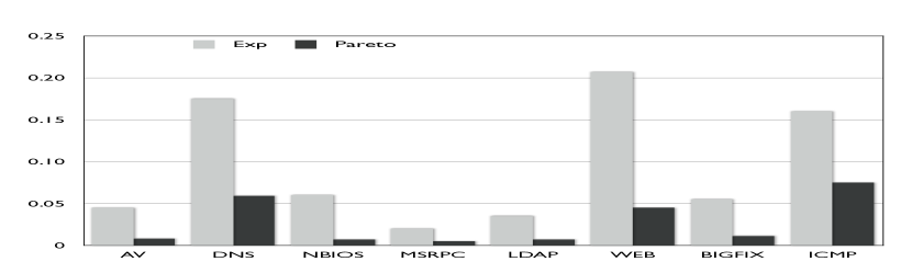
Figure 7: Flow counts across bins marked ’exp’ and ’pareto’

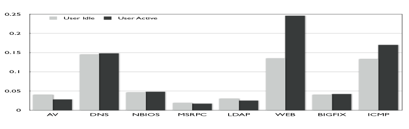
Figure 8: Flow counts in bins where user was idle/active

Fig. 8 plots the flow counts for a particular traffic category as it is observed in bins where the user is idle and when the user is active. Again, the counts were normalized by the total flow counts in each class. In this breakdown, we see that most of the traffic categories examined are present in equal measure whether the user is idle or active. On the one hand, the existence of a fair amount of heavy-tailed traffic during user-idle periods is somewhat surprising because it opposes findings from other heavy-tailed research studies claiming that user behavior is a cause of heavy-tailed traffic. On the other hand, it makes sense when you consider modern day practices for configuring enterprise clients. Such clients come pre-configured with security, monitoring and management software, which run autonomously and generate traffic that does not depend on user presence. We see that web traffic is the only category that differs substantially between user-active and user-idle time periods. The web traffic during user-idle periods may reflect web content that is refreshed aggressively, and also asynchronous (eg. AJAX) style applications.

While the results presented here are extremely preliminary, there is evidence that points to specific applications (and traffic types) contributing more to one part of the mixture model distribution. We plan to follow this direction in our future efforts.

VIII Conclusion

In this paper we set out to model flow traffic as generated by endhost machines such as enterprise employee laptops. We employ mixture models based on a convex combination of component distributions with both heavy and light-tails. We approach the modeling problem as a model selection problem rather than a goodness-of-fit test. Our methodology selects the best model for an endhost by considering a family of 3 models and doing pairwise comparisons to pick the best one. We employ the Bayes factor, based on the Bayesian Information Criteria (BIC), for these comparisons. To the best of our knowledge, this is the first paper to study heavy tails of data collected directly on endhosts, and is the first to employ a model selection approach.

We apply our methodology to data collected from 270 enterprise users, and find that for the vast majority of users, the methodology selects the EP model. Although there are some users best modeled by EEP, and few by P. This shows the importance of a method that users a family of distributions and does not presuppose a single distribution model for flow traffic. We learn that our enterprise user population contains a great deal of diversity; not only do different users need different models, but some are heavy-tailed and others not. We observe a wide range of values for the tail slope and mixing fraction in our models. We take an initial glance deeper into the network traffic and see hints that a small number of protocols and applications may be responsible for the observed heavy tail behavior. We also see the presence of heavy-tailed traffic when users are idle indicating that the flows comes from machine-generated traffic (such as enterprise applications and chatty protocols). In the future we plan to further explore the generative models behind the traffic patterns we observed herein.

References

- [1] Barford, P., Bestavros, A., Bradley, A., and Crovella, M. Changes in Web client access patterns: Characteristics and caching implications. World Wide Web (1999).
- [2] Barford, P., and Crovella, M. E. Generating representative Web workloads for network and server performance evaluation. In Proceedings of Performance ’98/SIGMETRICS ’98 (July 1998), pp. 151–160. Software for Surge is available from Mark Crovella’s home page.
- [3] Bharman, D., Chandrashekar, J., Taft, N., Faloutsos, M., Huang, L., and Giroire, F. Debating IT Monoculture for End Host Instrusion Detection. ACM Sigcomm Workshop on Research in Enterprise Networks (2009).
- [4] Breslau, L., Cue, P., Cao, P., Fan, L., Phillips, G., and Shenker, S. Web caching and zipf-like distributions: Evidence and implications. In In INFOCOM (1999), pp. 126–134.
- [5] Clauset, A., Shalizi, C. R., and Newman, M. E. J. Power-law distributions in empirical data. SIAM Review. To appear (2009).
- [6] Crovella, M. E., and Bestavros, A. Self-similarity in world wide web traffic: evidence and possible causes. IEEE/ACM Trans. on Networking 5, 6 (1997).
- [7] Crovella, M. E., and Taqqu, M. S. Estimating the heavy tail index from scaling properties. In Methodology and Computing in Applied Probability (1999), pp. 55–79.
- [8] Cunha, C. A., Bestavros, A., and Crovella, M. E. Characteristics of WWW client-based traces. Tech. Rep. TR-95-010, Boston University Department of Computer Science, Apr. 1995. Revised July 18, 1995.
- [9] Everitt, B. S., and Hand, D. J. Finite Mixture Distributions. Chapman and Hall, London, 1981.
- [10] Feldmann, A. Self-Similar Network Traffic and Performance Evaluation. Chapter 2: Characteristics of TCP Connection Arrivals. John Wiley & Sons, New York, NY, 2002.
- [11] Feldmann, A., Greenberg, A., Lund, C., Reingold, N., Rexford, J., and True, F. Deriving traffic demands for operational ip networks: Methodology and experience. IEEE/ACM Transactions on Networking 9 (2001), 265–279.
- [12] Feldmann, A., and Whitt, W. Fitting mixtures of exponentials to long-tail distributions to analyze network performance models. In Proceedings of IEEE INFOCOM’97 (April 1997).
- [13] Giroire, F., Chandrashekar, J., Iannaccone, G., Papagiannaki, K., Schooler, E., and Taft, N. The Cubicle Vs. The Coffee Shop: Behaviora Modes in Enterprise End-Users. Passive and Active Measurement Workshop (PAM) (2008).
- [14] Isdal, T., Piatek, M., Krishnamurthy, A., and Anderson, T. Leveraging BitTorrent for End Host Measurements. Passive and Active Measurement Workshop (PAM) (2007).
- [15] J. M. Marin, K. M., and Robert, C. Bayesian modelling and inference on mixtures of distributions. Tech. rep., CEREMADE, Universite Paris Dauphine, February 2004.
- [16] Jordan, M. I., and Jacobs, R. A. Hierachical mixtures of experts and the em algorithm. Neural Computation 6 (1994), 181–214.
- [17] Karagiannis, T., Mortier, R., and Rowstron, A. Network exception handlers: Host-network control in enterprise networks. ACM SIGCOMM (2008).
- [18] Kass, R. E., and Raftery, A. E. Bayes factors. Journal of the American Statistical Association 90, 430 (1995), 773–795.
- [19] Leland, W. E., Taqq, M. S., Willinger, W., and Wilson, D. V. On the self-similar nature of Ethernet traffic. In ACM SIGCOMM (San Francisco, California, 1993), D. P. Sidhu, Ed., pp. 183–193.
- [20] Li, L., Alderson, D., Willinger, W., and Doyle, J. C. A First-Principles Approach to Understanding the Internet’s Router-level Topology. Proc. ACM SIGCOMM (2004).
- [21] Luo, S., Li, J., Park, K., and Levy, R. Exploiting Heavy-Tailed Statistics for Predictable QoS Routing in Ad-Hoc Wireless Networks. IEEE Infocom (2008).
- [22] MacKay, D. J. C. Information Theory, Inference, and Learning Algorithms. Cambridge University Press, Cambridge, UK, 2003.
- [23] Newman, M. E. J. Power laws, pareto distributions and zipf’s law. Contemporary Physics 46, 5 (2005), p323 – 351.
- [24] Papagiannaki, K., Taft, N., and Diot, C. Impact of flow dynamics on traffic engineering design principles. In Proceedings of IEEE Infocom, Hong Kong, March 2004 (2004).
- [25] Paxson, V. Bro: A system for detecting network intruders in real-time. Computer Networks (1999).
- [26] Paxson, V., and Floyd, S. Wide-area traffic: the failure of poisson modeling. In SIGCOMM ’94: Proceedings of the conference on Communications architectures, protocols and applications (New York, NY, USA, 1994), ACM, pp. 257–268.
- [27] Resnick, S. I. Heavy-Tail Phenomena: Probabilistic and Statistical Modeling. Springer, 2007.
- [28] Simpson, C., Reddy, D., and Riley, G. Empirical Models of TCP and UDP End-User Network Traffic from NETI@home Data Analysis. Principles of Advanced and Distributed Simulation PADS (2006).
- [29] Tan, G., Poletto, M., Guttag, J., and Kaashoek, F. Role Classification of Hosts within Enterprise Networks Based on Connection Patterns. USENIX Annual Technical Conference (2003).
- [30] van der Vaart, A. W. Asymptotic Statistics (Cambridge Series in Statistical and Probabilistic Mathematics). Cambridge University Press, June 2000.
- [31] Wright, S. J. Primal-Dual Interior-Point Methods. SIAM Publications, 1997.