DELO-Bezier formal solutions of the polarized radiative transfer equation

Abstract

We present two new accurate and efficient method to compute the formal solution of the polarized radiative transfer equation. In this work, the source function and the absorption matrix are approximated using quadratic and cubic Bezier spline interpolants. These schemes provide 2${}^{\text{nd}}$ and 3${}^{\text{rd}}$ order approximation respectively and don’t suffer from erratic behavior of the polynomial approximation (overshooting). The accuracy and the convergence of the new method are studied along with other popular solutions of the radiative transfer equation, using stellar atmospheres with strong gradients in the line-of-sight velocity and in the magnetic-field vector.

1. Introduction

During the past decade, large scale numerical models and inverse problem applications became powerful tools for diagnosing and understanding spectroscopic and spectropolarimetric observations. Massive applications like 3D hydrodynamic (HD) simulations, Magnetic Doppler Imaging and data inversion of solar surface layers stimulated interest in developing fast and robust formal solvers for the radiative transfer equation (RTE). These computationally demanding problems pose special requirements for the RTE solver: a large number of integrations needed to compute synthetic profiles per single iterations (time step or model adjustment). Fast convergence become particularly important as it allows achieving acceptable accuracy for the radiation field using the same geometrical grid as used for hydrodynamics or inversion.

The properties of RTE solver become even more critical for non-equilibrium modeling. The assumption of local thermodynamic equilibrium (LTE) makes level population densities defined by the local temperature of the model and decoupled from the radiation field. Only one integration of the RTE is needed to compute the emerging intensity at each wavelength. However, in the non-LTE case (NLTE), evaluation of population densities is calculated using a self-consistent iterative method, normally requiring two integrations of the RTE per iteration (Olson & Kunasz, 1987). Inaccuracies in the integration of the RTE on a coarser grid can lead to a slower convergence of the NLTE problem in the spectral synthesis and generally to a slower convergence of the inversion (in LTE and NLTE). The situation is worse when the magnetic field becomes important.

The monochromatic radiative transfer equation for polarized light can be expressed as:

$$\frac{d\textbf{\em I}}{ds}=-\mathbf{K}\textbf{\em I}+\textbf{\em j}$$ (1)

where $\textbf{\em I}=(I,Q,U,V)^{T}$ is the Stokes parameter vector, $\textbf{\em j}=(j_{I},j_{Q},j_{U},j_{V})^{T}$  is the total emission vector, and $\mathbf{K}$ is the total absorption matrix. This matrix has seven independent terms: $\eta_{I}$ is the total absorption of radiation; $\eta_{Q}$, $\eta_{U}$ and $\eta_{V}$ describe the coupling of the intensity $I$ with $Q$, $U$ and $V$; and $\rho_{Q}$, $\rho_{U}$ and $\rho_{V}$ are cross-talk terms between $Q$, $U$ and $V$ due to magneto-optical effects (see Landi Degl’Innocenti & Landolfi, 2004):

$$\mathbf{K}=\begin{pmatrix}\eta_{I}&\eta_{Q}&\eta_{U}&\eta_{V}\\[3.00003pt] \eta_{Q}&\eta_{I}&\rho_{V}&-\rho_{U}\\[3.00003pt] \eta_{U}&-\rho_{V}&\eta_{I}&\rho_{Q}\\[3.00003pt] \eta_{V}&\rho_{U}&-\rho_{Q}&\eta_{I}\\[3.00003pt] \end{pmatrix}.$$ (2)

A number of advanced integration schemes, suitable for HD simulations and NLTE inversions have been implemented for the unpolarized light (Auer, 2003), however, for polarized light it is common to use a short characteristics schemes assuming linear (Rees et al., 1989) or parabolic dependence (Trujillo Bueno, 2003; Sampoorna et al., 2008) of the source function with optical path.

Bellot Rubio et al. (1998) proposed an efficient third-order method (LBR hereafter) that provides accurate results on coarse grids of depth-points for polarized light. This method has been used extensively to compute LTE inversions (Bellot Rubio et al., 2000; Socas-Navarro, 2011) and NLTE inversions (de la Cruz Rodríguez et al., 2012).

In this paper, we propose a new method to accurately integrate the polarized RTE, using Bezier interpolants. The paper is arranged as follows: an introduction to the DELO method and Bezier Splines are provided in § 2 and 3 respectively. For completeness, we introduce the solution to the unpolarized RTE, using Bezier interpolants, in § 4. The quadratic and cubic Bezier solutions to the polarized RTE are presented, for the first time, in § 5. Our proposed solutions are tested against other methods commonly used in radiative transfer studies in § 6. Finally, our conclusions are summarized in § 7.

2. The DELO method

Rees et al. (1989) rewrite the polarized RTE using the modified source vector ($\textbf{\em S}=\textbf{\em j}/\eta_{I}$), dividing all terms in Equation (1) by the absorption coefficient $\eta_{I}$. This simple change leaves the $\mathbf{K}$ matrix with all the diagonal elements normalized to one so the method got a name Diagonal Element Lambda Operator (DELO).

Defining,

$$\mathbf{\bar{K}}=\frac{\mathbf{K}}{\eta_{I}}-\mathbb{1},$$ (3)

where $\mathbb{1}$ is the $4\times 4$ identity matrix. The radiative transfer equation becomes:

$$\frac{d\textbf{\em I}}{d\tau_{\nu}}=\textbf{\em I}-\mathscrbf{S},$$ (4)

with the optical path defined as $d\tau_{\nu}=\eta_{I}ds$ and $\mathscrbf{S}=\textbf{\em S}-\mathbf{\bar{K}}\textbf{\em I}$.

In our discrete grid of $n$ depth points $(k=1,2,3,...,n)$, the solution to Equation (4) on the interval $(\tau_{k},\tau_{k+1})$ is:

$$\textbf{\em I}(\tau_{k})=\textbf{\em I}(\tau_{k+1})e^{-\delta_{k}}+\int_{\tau_{k}}^{\tau_{k+1}}e^{-(\tau-\tau_{k})}\mathscrbf{S}(\tau)d\tau,$$ (5)

where $\delta_{k}\equiv d\tau_{k}$.

To integrate analytically Equation (5), Rees et al. (1989) assume that the equivalent source vector $\mathscrbf{S}$ is linear with optical depth (conventionally referred to as DELO-linear). A quadratic dependence of $\mathscrbf{S}$ with optical depth would ideally allow to improve the convergence, however, it becomes unstable in the presence of non-linear gradients (Murphy, 1990).

3. The Bezier interpolants

Auer (2003) provides a thorough summary of advanced interpolants that could be used to integrate the (implicitly assumed) unpolarized radiative transfer equation.

3.1. Bezier quadratic interpolant

Defining normalized abscissa units in the interval $(x_{k},x_{k+1})$,

$$u=\frac{x-x_{k}}{x_{k+1}-x_{k}},$$ (6)

the quadratic Bezier interpolant can be expressed as:

$$f(x)=(1-u)^{2}y_{k}+y_{k+1}u^{2}+2u(1-u)\cdot C,$$ (7)

where $y_{k}$ and $y_{k+1}$ represent the node values of the function that is being interpolated and $C$ is the Bezier control point. The latter can be expressed using the derivative at $x_{k}$ or $x_{k+1}$,

$$C^{0}(x_{k}) = y_{k}+\frac{h_{k}}{2}y^{\prime}(x_{k}),$$ (8)

$$C^{1}(x_{k+1}) = y_{k+1}-\frac{h_{k}}{2}y^{\prime}(x_{k+1}),$$ (9)

with $h_{k}=x_{k+1}-x_{k}$. If both $C^{0}$ and $C^{1}$ can be computed, it is desirable to take the mean:

$$C=\left(C^{0}+C^{1}\right)/2,$$ (10)

resulting in a more ”symmetric” spline.

Defining,

$$\alpha=\frac{1}{3}\left(1+\frac{h_{k}}{h_{k}+h_{k-1}}\right),$$ (11)

$$d_{k+1/2}=\frac{y_{k+1}-y_{k}}{h_{k}},$$ (12)

$$d_{k-1/2}=\frac{y_{k}-y_{k-1}}{h_{k-1}},$$ (13)

accurate numerical derivatives are calculated at the node points $(x_{1,2,...,n})$ with a scheme that suppresses overshooting beyond the node function values (Fritsch & Butland, 1984). The Bezier derivative is given by:

$$y^{\prime}(x_{i})=\frac{d_{i-1/2}\cdot d_{i+1/2}}{\alpha\cdot d_{i+1/2}+(1-\alpha)\cdot d_{i-1/2}},$$ (14)

if $d_{k-1/2}\cdot d_{k+1/2}>0$ and it is set to 0 otherwise.

3.2. Bezier cubic interpolant

Alternatively, the cubic Bezier interpolant can be expressed as:

$$\begin{split}f(x)=&(1-u)^{3}y_{k}+y_{k+1}u^{3}+\\ &3u(1-u)^{2}\cdot\hat{E}+3u^{2}(1-u)\cdot\hat{F},\end{split}$$ (15)

where $\hat{E}$ and $\hat{F}$ are control points, similar to those defined in Equations (8) and (9), but each of them is placed in a different location:

$$\hat{E}(x_{k}) = y_{k}+\frac{h_{k}}{3}y^{\prime}(x_{k}),$$ (16)

$$\hat{F}(x_{k+1}) = y_{k+1}-\frac{h_{k}}{3}y^{\prime}(x_{k+1}).$$ (17)

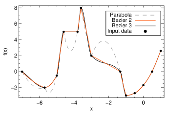
Figure 1.— Comparison of 3 interpolation schemes. The black circles indicate the know values of the function that is interpolated using quadratic Bezier spline, cubic Bezier spline and piece-wise parabolic fit.

Fig. 1 illustrates the behavior of three interpolation schemes, when the function has fast changing gradient. Here, we compare a parabolic polynomial, the quadratic Bezier splines (Bezier 2) and the cubic Bezier splines (Bezier 3) described in this section.

The behavior of the parabolic fit is erratic in the vicinity of intervals with large change of gradient, showing dramatic overshooting peaks. The Bezier splines considered here stays between the pair of boundary data values in each interval. If fact, Auer (2003) already suggested that the Bezier splines (and the Hermitian interpolant) are particularly suitable for solving the radiative transfer equation in form (5) as they do not produce spurious maxima and minima.

From $x=-1$ to $x=1$ the curve increases smoothly, and the three interpolation schemes considered here produce very similar values.

4. Bezier integration of the scalar RTE

In this section, we derive the formal solution of the radiative transfer equation for unpolarized light $(\mathbf{\bar{K}}=0)$. In this case Equation (4) becomes a scalar equation:

$$\frac{dI}{d\tau}=I-S,$$ (18)

where $I$ is the intensity and $S$ is the unpolarized source function. Equation (5) is easily integrated by approximating $S$ with any of the Bezier interpolants described in Sec. 3.

4.1. Quadratic Bezier integration

If the quadratic Bezier interpolant is used to approximate the source function, the solution to Equation (5) is

$$I(\tau_{k})=I(\tau_{k+1})\cdot e^{-\delta_{k}}+\alpha_{k}S_{k}+\beta_{k}S_{k+1}+\gamma_{k}C_{k},$$ (19)

where $\alpha_{k}$, $\beta_{k}$ and $\gamma_{k}$ are coefficients from the integral that only depend on $\delta_{k}\equiv\tau_{k+1}-\tau_{k}$:

$$\alpha_{k} = \frac{2+\delta^{2}_{k}-2\delta_{k}-2e^{-\delta_{k}}}{\delta^{2}_{k}},$$

$$\beta_{k} = \frac{2-(2+2\delta_{k}+\delta_{k}^{2})e^{-\delta_{k}}}{\delta_{k}^{2}},$$

$$\gamma_{k} = \frac{2\delta_{k}-4+(2\delta_{k}+4)e^{-\delta_{k}}}{\delta_{k}^{2}}.$$

To calculate $\delta_{k}$, the opacity can be integrated analytically by using Bezier splines to approximate $\eta_{I}$ as a function of depth. Further details can be found in Appendix A.

Note, that for small $\delta_{k}$ it is wise to use Taylor expansion for the exponents in the right-hand-side to avoid division of vanishingly small quantities (see Appendix B).

Equation (19) has the form $I_{k}=A\cdot I_{k+1}+B$. In the case of a stellar atmosphere we can sequentially evaluate outgoing intensity at any depth point starting from the boundary condition $I_{n}=S_{n}$ at the bottom. The control point $C_{k}$ is computed using Equation (10) for all inner points of the integration domain. For the top point only one approximation for the control point ($C^{1}$) is available.

4.2. Cubic Bezier integration

If the cubic Bezier interpolant is used to approximate the source function, the solution to Equation (5) is

$$\begin{split}I(\tau_{k})=&I(\tau_{k+1})\cdot e^{-\delta_{k}}+\hat{\alpha}_{k}S_{k}+\hat{\beta}_{k}S_{k+1}\\ &+\hat{\gamma}_{k}\hat{E}_{k}+\hat{\epsilon}_{k}\hat{F}_{k}.\end{split}$$ (20)

$\hat{\alpha}_{k}$, $\hat{\beta}_{k}$, $\hat{\gamma}_{k}$, $\hat{\epsilon}_{k}$ are coefficients from the integral that only depend on $\delta_{k}$:

$$\hat{\alpha}_{k} = \frac{-6+6\delta_{k}-3\delta_{k}^{2}+\delta_{k}^{3}+6e^{-\delta_{k}}}{\delta_{k}^{3}},$$

$$\hat{\beta}_{k} = \frac{6+(-6-\delta_{k}(6+\delta_{k}(3+\delta_{k})))\cdot e^{-\delta_{k}}}{\delta_{k}^{3}},$$

$$\hat{\gamma}_{k} = 3\cdot\frac{6+(\delta_{k}-4)\delta_{k}-2(\delta_{k}+3)\cdot e^{-\delta_{k}}}{\delta_{k}^{3}},$$

$$\hat{\epsilon}_{k} = 3\cdot\frac{2\delta_{k}-6+(6+\delta_{k}^{2}+4\delta_{k})\cdot e^{-\delta_{k}}}{\delta_{k}^{3}}.$$

The same recommendations apply here for small $\delta_{k}$.

5. Bezier Integration of the vector RTE

5.1. Quadratic Bezier integration

For the polarized case $(\mathbf{\bar{K}}\neq 0)$, the solution to Equation (5) can formally be presented in the form similar to Equation (19):

$$\textbf{\em I}(\tau_{k}) = \textbf{\em I}(\tau_{k+1})\cdot e^{-\delta_{k}}+\alpha_{k}\mathscrbf{S}(\tau_{k})+$$ (21)

$$+ \beta_{k}\mathscrbf{S}(\tau_{k+1})+\gamma_{k}\textbf{\em C}_{k}.$$

In Sec. 4, Equation (14) we show how to compute the derivatives of $S$ needed for evaluating the control point $C$. In the polarized case, however, derivatives of I, S and $\mathbf{\bar{K}}$ must be computed. The presence of $\textbf{\em I}_{k}$ in the denominators of both $C^{0}$ and $C^{1}$ (through Equation (14)) introduces non-linearity that kills a simple recurrence relation available in the scalar case: $\textbf{\em I}_{k}=\mathbf{A}\cdot\textbf{\em I}_{k+1}+\textbf{\em B}$.

An elegant solution to this problem is actually provided by the radiative transfer equation:

$$\textbf{\em I}^{\prime}_{k} = \textbf{\em I}_{k}-\textbf{\em S}_{k}+\mathbf{\bar{K}}_{k}\textbf{\em I}_{k},$$ (22)

$$\textbf{\em I}^{\prime}_{k+1} = \textbf{\em I}_{k+1}-\textbf{\em S}_{k+1}+\mathbf{\bar{K}}_{k+1}\textbf{\em I}_{k+1}.$$ (23)

Using these expressions, the control points can be re-written as:

$$\begin{split}\textbf{\em C}^{0}_{k}=&\overbrace{\left(\mathbb{1}+\frac{\delta_{k}}{2}\mathbf{\bar{K}}_{k}\right)\textbf{\em S}_{k}+\frac{\delta_{k}}{2}\textbf{\em S}^{\prime}_{k}}^{\textbf{\em c}_{k}^{0}}-\\ &\underbrace{-\left[\frac{\delta_{k}}{2}\left(\mathbf{\bar{K}}_{k}\mathbf{\bar{K}}_{k}+\mathbf{\bar{K}}^{\prime}_{k}+\mathbf{\bar{K}}_{k}\right)+\mathbf{\bar{K}}_{k}\right]}_{\bar{\mathbf{c}}_{k}^{0}}\textbf{\em I}_{k}=\\ =&\ \textbf{\em c}_{k}^{0}+\mathbf{\bar{c}}_{k}^{0}\textbf{\em I}_{k},\end{split}$$ (24)

and:

$$\begin{split}\textbf{\em C}^{1}_{k}=&\left(\mathbb{1}-\frac{\delta_{k}}{2}\mathbf{\bar{K}}_{k+1}\right)\textbf{\em S}_{k+1}-\frac{\delta_{k}}{2}\textbf{\em S}^{\prime}_{k+1}+\\ +&\left[\frac{\delta_{k}}{2}\left(\mathbf{\bar{K}}_{k+1}\mathbf{\bar{K}}_{k+1}+\mathbf{\bar{K}}^{\prime}_{k+1}+\mathbf{\bar{K}}_{k+1}\right)\right.-\\ -&\left.\mathbf{\bar{K}}_{k+1}\right]\textbf{\em I}_{k+1}.\end{split}$$ (25)

Note that $\textbf{\em C}^{1}_{k}$ and $\textbf{\em c}_{k}^{0}$ are vectors, whereas $\mathbf{\bar{c}}_{k}^{0}$ is a matrix.

The derivatives of the modified opacity matrix $\mathbf{\bar{K}}^{\prime}$ and the source vector $\textbf{\em S}^{\prime}$ must be computed according to the recipe for monotonicity given by Equations (11)-(14) to prevent the overshooting.

This convenient splitting of $\textbf{\em C}^{0}$ permits re-writing Equation (21) for unknown Stokes vector in point $k$ as a system of four linear equations $(\mathbf{A}\cdot\textbf{\em I}_{k}\leavevmode\nobreak\ =\leavevmode\nobreak\ \textbf{\em B})$:

$$\underbrace{\left(\mathbb{1}+\alpha_{k}\mathbf{\bar{K}}_{k}-\frac{\gamma_{k}}{2}\mathbf{\bar{c}}_{k}^{0}\right)}_{\mathbf{A}}\textbf{\em I}_{k}=\underbrace{\boldsymbol{\xi}_{k}+\frac{\gamma_{k}}{2}(\textbf{\em C}_{k}^{1}+\textbf{\em c}_{k}^{0})}_{\textbf{\em B}},$$ (26)

with,

$$\boldsymbol{\xi}_{k}=\textbf{\em I}_{k+1}e^{-\delta_{k}}+\alpha_{k}\textbf{\em S}_{k}+\beta_{k}\mathscrbf{S}_{k+1}.$$ (27)

Note, that the matrix and the right-hand-side in Equation 26, include only known quantities of absorption matrix, source and Stokes vectors. Note also, that solving the system of linear equations (26) directly instead of trying to invert A is both faster and more robust.

5.2. Cubic Bezier integration

Similarly to the quadratic Bezier integration, the solution to Equation (5) is formally similar to Equation (20):

$$\textbf{\em I}(\tau_{k}) = \textbf{\em I}(\tau_{k+1})\cdot e^{-\delta_{k}}+\hat{\alpha}_{k}\mathscrbf{S}(\tau_{k})+$$ (28)

$$+ \hat{\beta}_{k}\mathscrbf{S}(\tau_{k+1})+\hat{\gamma}_{k}\hat{\textbf{\em E}}_{k}+\hat{\epsilon}_{k}\hat{\textbf{\em F}}_{k}.$$

Given the formal similarity of this equation with the quadratic case, where also two control points are used, the algebra needed to write the problem as a linear system of equations (Equation (26)) is almost identical.

$$\begin{split}\hat{\textbf{\em E}}_{k}=&\overbrace{\left(\mathbb{1}+\frac{\delta_{k}}{3}\mathbf{\bar{K}}_{k}\right)\textbf{\em S}_{k}+\frac{\delta_{k}}{3}\textbf{\em S}^{\prime}_{k}}^{\textbf{\em e}_{k}}-\\ &\underbrace{-\left[\frac{\delta_{k}}{3}\left(\mathbf{\bar{K}}_{k}\mathbf{\bar{K}}_{k}+\mathbf{\bar{K}}^{\prime}_{k}+\mathbf{\bar{K}}_{k}\right)+\mathbf{\bar{K}}_{k}\right]}_{\bar{\mathbf{e}}_{k}}\textbf{\em I}_{k}=\\ =&\ \textbf{\em e}_{k}+\mathbf{\bar{e}}_{k}\textbf{\em I}_{k},\end{split}$$ (29)

and:

$$\begin{split}\hat{\textbf{\em F}}_{k}=&\left(\mathbb{1}-\frac{\delta_{k}}{3}\mathbf{\bar{K}}_{k+1}\right)\textbf{\em S}_{k+1}-\frac{\delta_{k}}{3}\textbf{\em S}^{\prime}_{k+1}+\\ +&\left[\frac{\delta_{k}}{3}\left(\mathbf{\bar{K}}_{k+1}\mathbf{\bar{K}}_{k+1}+\mathbf{\bar{K}}^{\prime}_{k+1}+\mathbf{\bar{K}}_{k+1}\right)\right.-\\ -&\left.\mathbf{\bar{K}}_{k+1}\right]\textbf{\em I}_{k+1}.\end{split}$$ (30)

Equation (28) can be re-arranged to group all the terms containing $\textbf{\em I}(\tau_{k})$ on the left-hand side of the equation.

$$\begin{split}&\underbrace{\left(\mathbb{1}+\hat{\alpha}_{k}\mathbf{\bar{K}}_{k}-\hat{\gamma}_{k}\mathbf{\bar{e}}_{k}\right)}_{\mathbf{A}}\textbf{\em I}_{k}=\\ &=\underbrace{\textbf{\em I}_{k+1}e^{-\delta_{k}}+\hat{\alpha}_{k}\textbf{\em S}_{k}+\hat{\beta}_{k}\mathscrbf{S}_{k+1}+\hat{\gamma}_{k}\textbf{\em e}_{k}+\hat{\epsilon}_{k}\hat{\textbf{\em F}}_{k}}_{\textbf{\em B}}.\end{split}$$ (31)

Again we advise to solve the linear system of equations in Equation (31), instead of inverting the A matrix.

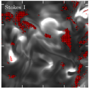
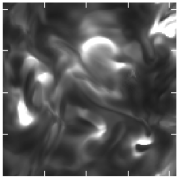
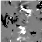
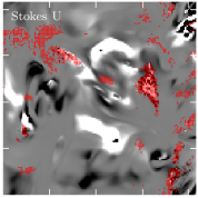
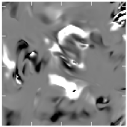
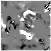
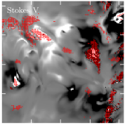
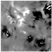
Figure 2.— Monochromatic full-Stokes images computed at the core of the Ca II $\lambda 8542$ line. From left to right, the images are computed using the DELO-parabolic, DELO-linear, DELO-Bezier and cubic DELO-Bezier, respectively. Stokes $I$, $Q$, $U$ and $V$ are represented from top to bottom respectively. Regions with artifacts are marked in the panels computed using the DELO-par method using small red squares.

6. Numerical calculations

We use a modified version of the radiative transfer code Nicole (Socas-Navarro et al. in prep), to test the numerical accuracy of the DELO-Bezier methods for polarized light. A snapshot from a 3D MHD numerical simulation is used to carry-out the calculation of synthetic full-stokes profiles. It covers a physical range of $16.6\times 8.3\times 15.5$ Mm, extending from the upper convection zone to the lower corona (from 1.5 Mm below to 14 Mm above average optical depth unity at 5000 Å). The simulation has an average magnetic field strength of 150 G in the photosphere. This particular snapshot has been used by Leenaarts et al. (2009); de la Cruz Rodríguez et al. (2012) so further details on simulations can be found there.

6.1. The NLTE problem

As described in de la Cruz Rodríguez et al. (2012), the Nicole code solves the NLTE problem for unpolarized light (Socas-Navarro & Trujillo Bueno, 1997) and, once the atom population densities are known, a polarized formal solution is calculated (the polarization-free approximation, see Trujillo Bueno & Landi Degl’Innocenti, 1996). The Ca II atom model used in this work consists of five bound levels plus a continuum.

Additionally, the velocity-free approximation, previously used to compute the data inversions in Socas-Navarro et al. (2000); de la Cruz Rodríguez et al. (2012), is not used in this study. Therefore the population densities are fully consistent with the strong velocity gradients present in our models.

For consistency, we have implemented an accelerated local lambda operator based in the unpolarized solution described in Sec. 4.

The process of constructing the approximate lambda operator at any given point $k$, can be idealized by setting the source function to unity in that point, and zero otherwise. The operator is constructed using the terms from Equation (19) that remain after this operation (Olson & Kunasz, 1987).

According to Equation (10), the average control point $C$ has an explicit dependency on $C^{0}_{k}(S_{k})$ and $C^{1}_{k}(S_{k+1})$. Using the average of the two $C$’s improves stability and accuracy of the Bezier interpolant, although the lambda operator becomes intrinsically non local.

A simple recipe for reducing the number of iterations for the NLTE problem is to make the approximate lambda operator strictly local by setting $C=C^{0}_{k}$. Rare cases of minor overshooting are suppressed by forcing the control point $\text{min}(S_{k},S_{k+1})\leq C_{k}\leq\text{max}(S_{k},S_{k+1})$. Similar strategies are found in Hayek et al. (2010) and Holzreuter & Solanki (2012).

We used the approximate lambda operator for solving the NLTE problem in the form:

$$\Lambda^{*}_{k}=r_{\nu\mu}(\alpha_{k}+\gamma_{k}),$$ (32)

where $r_{\nu\mu}$ is the ratio between the line opacity and the total opacity (see Rybicki & Hummer, 1991, for further details).

Fig. 2 illustrates the full-Stokes images at the surface of a $8.3\times 8.3$ Mm patch computed at $-10$ mÅ from the core of the Ca II $\lambda 8542$ line. Columns of panels (from left to right) show the monochromatic images obtained using DELO-parabolic, DELO-linear, quadratic DELO-Bezier and cubic DELO-Bezier, respectively. We used identical NLTE level populations to compute the polarized formal solution with each algorithm. Thus, the differences between panels in different columns reflect the numerical properties (convergence and stability) of the methods compared.

The DELO-parabolic method seems to work in most of the pixels, but it fails notoriously to produce an accurate solution at certain areas which have been indicated on the panels using red markers. The artifacts here can be quite large, and some pixels show even negative values in Stokes $I$.

The maximum difference in Stokes $I$ between DELO-linear and DELO-Beziers at this wavelength is less than $1\%$ of the continuum intensity. This is an expected result, given that the vertical grid spacing of 3D snapshots is so fine that even a linear scheme produces an accurate solution.

This example only shows the stability of the higher-order Bezier methods, but it hardly shows any advantage over a linear scheme.

In Sec. 6.2 we test the converges and stability of these methods using 1D models where strong gradients in the magnetic-field and line-of-sight (l.o.s) velocity are introduced.

6.2. Numerical accuracy

To assess the accuracy of the formal solvers, we have created four atmospheric models using a fine grid of depth-points with 198 points-per-decade, equidistantly placed from $\log\tau_{500}=-6.9$ to $\log\tau_{500}=2$.

The four atmospheric models share the same temperature, electron pressure, and micro-turbulence from the VALC-III model (Vernazza et al., 1981).

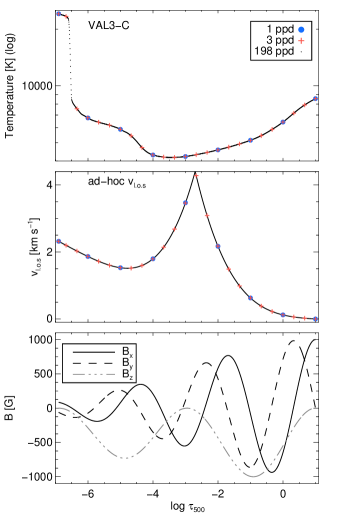
Figure 3.— Physical quantities from our prescribed 1D stellar model. The top panel shows the temperature stratification as a function of optical depth. The middle panel shows an ad-hoc profile used to define $v_{l.o.s}$ in our calculations. The bottom panel illustrates the three components of the magnetic field. To illustrate the effects of having a poor sampling in the vertical dimension, we have marked in the first two panels, the equivalent model assuming 1 point-per-decade (blue circles), 3 points-per-decade (red crosses) and 198 points-per-decade (black dots). Note that the $z$-axis is parallel to the line-of-sight.

We have created a complicated ad-hoc magnetic field vector and l.o.s velocity component, which are illustrated in Fig. 3, along with the VALC-III temperature. To create a demanding topology, the horizontal component of the magnetic-field follows a spiral centered on the line-of-sight.

Considering the quantities described above, our set of four models is summarized as follows:

1. The first case is a model with constant l.o.s velocity ($v_{l.o.s}=0$ km s^-1) and constant magnetic-field $\textbf{\em B}=(600,-700,800)$ G for all depth-points.

2. In the second case, the constant line-of-sight velocity is replaced with our ad-hoc profile.

3. The third case has constant velocity but the complicated magnetic-field vector described in Fig. 3.

4. Complex velocity and magnetic-field profiles are used simultaneously in the fourth case.

For each of these four cases, we have computed the absorption matrix and the source function in the original grid of depth-points for the Ca II $\lambda 8542$ and the Fe I $\lambda 6302$ lines. These two lines have been extensively used as atmospheric diagnostics in solar applications. The former is sensitive to a vast range of height including photospheric and chromospheric response, although it has an relatively low Landé factor ($g_{\text{eff}}=1.1$). The latter is formed in the solar photosphere, but it has a much higher sensitivity to the magnetic-field ($g_{\text{eff}}=2.5$).

Our test consists of computing the formal solution to the polarized RTE using a pre-computed absorption matrix and source function. To study the converge properties of the integrators we simply drop intermediate depth-points from the original grid. Thus we separate the level population calculations from the RTE solution. We also noticed that our level population calculations for Ca II start deviating noticeably from the correct solution when the number of depth-points is below 10 points-per-decade.

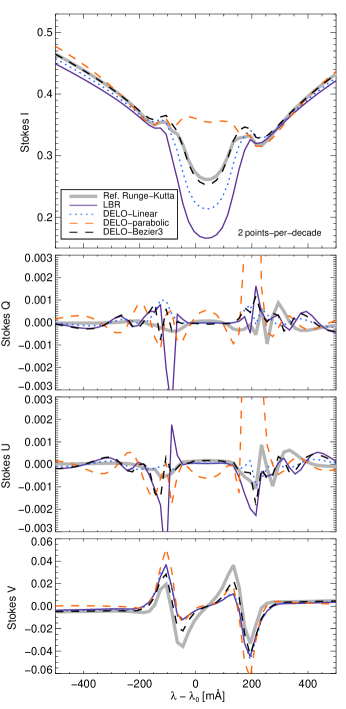
Figure 4.— Emerging intensity vector at the Ca II $\lambda 8542$ line. The profiles are computed using our fourth model which contains gradients in the magnetic-field and line-of-sight-velocity. The model here has a vertical resolution of of 2 points-per-decade. The reference profile is computed using a Runge-Kutta solver using the original grid of 198 points-per-decade. For readability, only the cubic DELO-Bezier solution is plotted.

As a reference here we use the emerging Stokes vector computed on the original grid of 198 points-per-decade, using an adaptive fourth-order Runge-Kutta solver (see Landi Degl’Innocenti, 1976), which ensures that the precision of $10^{-13}$ as achieved at every step.

Fig. 4 shows a set of Stokes $I$, $Q$, $U$ and $V$ profiles computed for the complex of our ad-hoc models (model 4) using a 2 points-per-decade grid. The reference grey profile has been computed using the Runge-Kutta method and the original dense grid of depth-points. The main discrepancies occur at the chromospheric NLTE core of the Ca II $\lambda 8542$ line. At those wavelengths, the monochromatic depth-scale presents large irregular jumps in optical-depth.

For example, in Stokes $I$ the LBR and DELO-linear solutions present an excessively strong line core, whereas the DELO-parabolic method produces a line core in emission. The DELO-Bezier profiles tightly trace the reference profile at all wavelengths, and only a noticeable small deviation is present at the very inner core of the line.

The results of our calculations are summarized in Fig. 5 and Fig. 6, for the Ca II $\lambda 8542$ line and the Fe I $\lambda 6302$ line respectively. The line profiles are compared with the reference case, and the largest discrepancy over the entire profile (in absolute value) is plotted for each integration method as a function of the number of depth-points per decade.

This error measurement is sensitive to outliers at a single wavelength. Therefore, the curves in Fig. 5 and Fig. 6 may not be monotonous functions of the number of grid points. Still, we prefer this metric as it gives a robust estimate of accuracy, convergence speed and stability for our solvers.

Ideally, we would expect that any discrepancies shown by all the methods considered here, would disappear when the density of depth-points is large enough (all methods should converge to the same accurate solution). The errors are expected to be large when the density of depth-points is low, especially for the highest order methods, but these should achieve a more accurate solution than the lower order methods when the density of depth-points is relatively high.

In Fig. 5, our results show that at the absolute minimum of 1 points-per-decade, it is hard to beat the DELO-linear solution, which keep the errors under control despite the strong gradients and poorly-sampled stellar atmosphere. However, the DELO-Bezier solutions provide almost as accurate results except in Stokes $Q$ where the error is half an order of magnitude higher.

The situation changes drastically, as a few more depth-points are included in the calculations. Between five and thirty points-per-decade, the DELO-Bezier solutions clearly out-perform all the other solutions for the four scenarios that we have prepared. Most radiative transfer computations are carried out within this range of grid densities. This also matches hydrodynamic grid density typically used for environments where radiation carries important fraction of energy.

The DELO-parabolic needs a large number of depth-points to match the performance of all the other methods, as was expected.

The calculations for the Fe I $\lambda 6302$ line, show a smoother behavior than in the previous case and all cases seem to reach a stable level of accuracy at approximately 30 points-per-decade. The inclusion of more points above this value, seems to increase the accuracy marginally and very inefficiently.

The DELO-Bezier demonstrated fastest convergence reaching below 10 %  for the least dense grids in Stokes $I$. This conclusion is true for all our models. The accuracy of all methods is comparable as they all reach the same level of precision above 30 points-per-decade.

For both spectral lines, the performance of the LBR method is close to both the DELO-linear and DELO-parabolic methods, and it only seems to be slightly less accurate when strong gradients in the line-of-sight velocity are present.

The accuracy achieved by the DELO-Bezier methods is almost identical. The quadratic solution marginally outperforms the cubic one when the number of depth-points per decade is 1 or 2, whereas the cubic version is slightly better at the Ca II $\lambda 8542$ line, within the range $2<\text{N}_{\text{depth}}<10$ points-per-decade.

Computationally, the LBR and DELO-Bezier solutions are similarly demanding given that accurate derivatives of the source function and of the absorption matrix are required. In comparison, the DELO-linear and DELO-parabolic solutions are almost two times faster, because no derivatives are required.

Note also that, in the first and last intervals of the grid, only one control-point can be computed. Therefore, especial care must be taken when the cubic method is used. The simplest solution is to use the quadratic method in those two intervals, given that only one control point is strictly necessary.

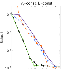
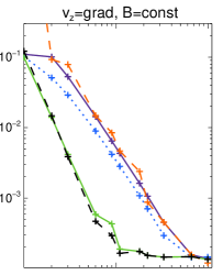
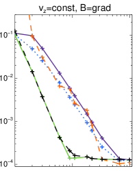
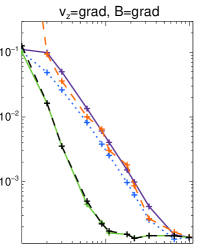
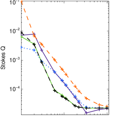
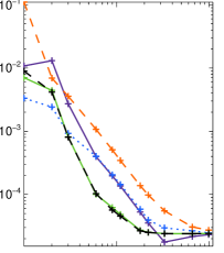
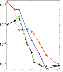
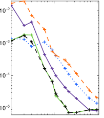
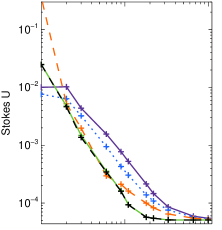
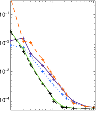
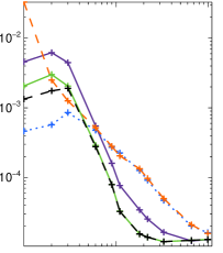
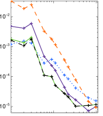
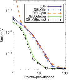
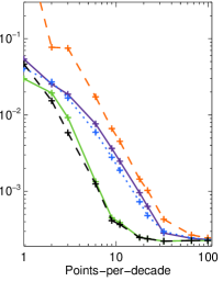
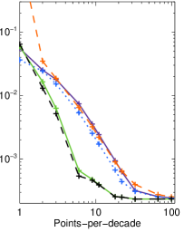
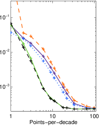
Figure 5.— Maximum error for the Ca II $\lambda 8542$ line as a function of the number of points-per-decade (at all wavelengths). From top to bottom, the panels show the errors for Stokes $I$, $Q$, $U$ and $V$, respectively. From left to right, each column corresponds to each of the four models used in our calculations. Each colored line corresponds to one of the formal solutions used in our calculations: LBR (solid purple), DELO-linear (dotted blue), DELO-parabolic (dashed orange), quadratic DELO-Bezier (solid green) and cubic DELO-Bezier (dashed black).

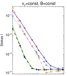
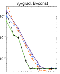
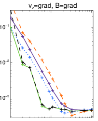
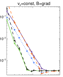
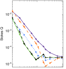
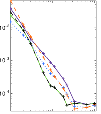
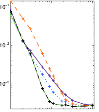
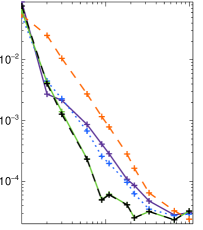
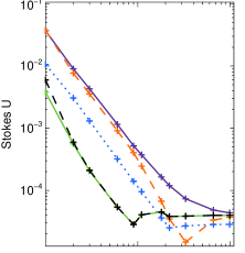
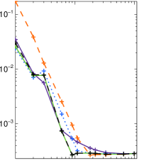
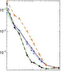
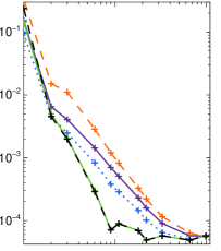
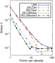
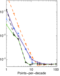
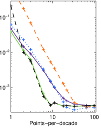
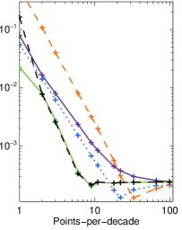
Figure 6.— Maximum error for the Fe I $\lambda 6302$ line as a function of the number of points-per-decade (at all wavelengths). From top to bottom, the panels show the errors for Stokes $I$, $Q$, $U$ and $V$, respectively. From left to right, each column corresponds to each of the four models used in our calculations. Each colored line corresponds to one of the formal solutions used in our calculations: LBR (solid purple), DELO-linear (dotted blue), DELO-parabolic (dashed orange), quadratic DELO-Bezier (solid green) and cubic DELO-Bezier (dashed black).

7. Discussion and conclusions

In this work we present a new scheme to integrate the polarized radiative transfer equation using Bezier splines. The solvers are a generalization of the advanced strategy proposed by Auer (2003) for the unpolarized case. Our second-order and third-order integration methods preserve the stability of the DELO-linear solution with the benefits of faster convergence and higher order accuracy.

The advantages of the new integration scheme are illustrated by comparison with other methods commonly used to solve the polarized RTE. We show that the new DELO-Bezier schemes outperform all other algorithms when the density of depth-points is low and the structure of the medium includes steep gradients.

The new methods will be beneficial for various application from reconstructing atmospheric structure(s) using observational data (data inversion in solar physics, Magnetic Doppler Imaging of stars) to radiative magneto-hydrodynamics. E.g., in case of solar data inversion the new solvers will allow using less denser depth grid improving the stability of inversion, which is particularly important for strong lines, like the Ca II H,K and the IR triplet. Given the vast formation range of these lines (larger than $1000$ km), it is hard to find an optimal grid of depth points at all frequencies in the line.

Appendix A Bezier integral of the opacity

In many radiative transfer applications, a conversion of the depth-scale is desirable (i.e, from $z$ to $\log\tau_{500}$). To carry out this conversion, the opacity ($\eta_{I}\equiv\eta$) is integrated along the depth-scale. When the grid of depth-points is sufficiently dense, a trapezoidal integration would suffice. This wide-spread method becomes inaccurate for coarse depth-scale grids.

We advice to approximate the opacity with a quadratic Bezier spline (Eq. 7), and integrate analytically this function. Once again, the integral can be expressed as a set of coefficients that multiply the values of the opacity that define the integration interval:

$$\begin{split}d\tau_{k}(\nu)=\tau_{k+1}-\tau_{k}=&(x_{k+1}-x_{k})\int^{1}_{0}\left[\eta_{k}(\nu)*(1-u)^{2}+\eta_{k+1}(\nu)*u^{2}+2u(1-u)C\right]du=\\ =&\frac{x_{k+1}-x_{k}}{3}\left(\eta_{k}(\nu)+\eta_{k+1}(\nu)+C\right).\end{split}$$ (A1)

Appendix B Taylor expansion of the Bezier integral coefficients

In § 4 we advise to use a Taylor expansion of the exponential term in Equation (5), when $\delta_{k}$ is small:

$$e^{-\delta_{k}u}\approx 1-\delta_{k}u+\frac{\delta_{k}^{2}u^{2}}{2}-\frac{\delta_{k}^{3}u^{3}}{6}.$$

The resulting integration coefficients for the quadratic Bezier interpolant are:

$$\alpha_{k} = \frac{\delta_{k}}{3}-\frac{\delta_{k}^{2}}{12}+\frac{\delta_{k}^{3}}{60},$$

$$\beta_{k} = \frac{\delta_{k}}{3}-\frac{\delta_{k}^{2}}{4}+\frac{\delta_{k}^{3}}{10},$$

$$\gamma_{k} = \frac{\delta_{k}}{3}-\frac{\delta_{k}^{2}}{6}+\frac{\delta_{k}^{3}}{20}.$$

The integration coefficients for the cubic Bezier interpolant are:

$$\hat{\alpha_{k}} = \frac{\delta_{k}}{4}-\frac{\delta_{k}^{2}}{20}+\frac{\delta_{k}^{3}}{120}-\frac{\delta_{k}^{4}}{840},$$

$$\hat{\beta_{k}} = \frac{\delta_{k}}{4}-\frac{\delta_{k}^{2}}{5}+\frac{\delta_{k}^{3}}{12}-\frac{\delta_{k}^{4}}{42},$$

$$\hat{\gamma_{k}} = \frac{\delta_{k}}{4}-\frac{\delta_{k}^{2}}{10}+\frac{\delta_{k}^{3}}{40}-\frac{\delta_{k}^{4}}{210},$$

$$\hat{\epsilon_{k}} = \frac{\delta_{k}}{4}-\frac{3\delta_{k}^{2}}{20}+\frac{\delta_{k}^{3}}{20}-\frac{\delta_{k}^{4}}{84}.$$

References

- Auer (2003) Auer, L. 2003, in Astronomical Society of the Pacific Conference Series, Vol. 288, Stellar Atmosphere Modeling, ed. I. Hubeny, D. Mihalas, & K. Werner, 3
- Bellot Rubio et al. (1998) Bellot Rubio, L. R., Ruiz Cobo, B., & Collados, M. 1998, ApJ, 506, 805
- Bellot Rubio et al. (2000) —. 2000, ApJ, 535, 475
- de la Cruz Rodríguez et al. (2012) de la Cruz Rodríguez, J., Socas-Navarro, H., Carlsson, M., & Leenaarts, J. 2012, A&A, 543, A34
- Fritsch & Butland (1984) Fritsch, F. N., & Butland, J. 1984, j-SIAM-J-SCI-STAT-COMP, 5, 300
- Hayek et al. (2010) Hayek, W., Asplund, M., Carlsson, M., Trampedach, R., Collet, R., Gudiksen, B. V., Hansteen, V. H., & Leenaarts, J. 2010, A&A, 517, A49
- Holzreuter & Solanki (2012) Holzreuter, R., & Solanki, S. K. 2012, A&A, 547, A46
- Landi Degl’Innocenti (1976) Landi Degl’Innocenti, E. 1976, A&AS, 25, 379
- Landi Degl’Innocenti & Landolfi (2004) Landi Degl’Innocenti, E., & Landolfi, M., eds. 2004, Astrophysics and Space Science Library, Vol. 307, Polarization in Spectral Lines
- Leenaarts et al. (2009) Leenaarts, J., Carlsson, M., Hansteen, V., & Rouppe van der Voort, L. 2009, ApJ, 694, L128
- Murphy (1990) Murphy, G. A. 1990, PhD thesis, , Univ. Sidney, (1990)
- Olson & Kunasz (1987) Olson, G. L., & Kunasz, P. B. 1987, J. Quant. Spec. Radiat. Transf., 38, 325
- Rees et al. (1989) Rees, D. E., Durrant, C. J., & Murphy, G. A. 1989, ApJ, 339, 1093
- Rybicki & Hummer (1991) Rybicki, G. B., & Hummer, D. G. 1991, A&A, 245, 171
- Sampoorna et al. (2008) Sampoorna, M., Nagendra, K. N., & Stenflo, J. O. 2008, ApJ, 679, 889
- Socas-Navarro (2011) Socas-Navarro, H. 2011, A&A, 529, A37
- Socas-Navarro & Trujillo Bueno (1997) Socas-Navarro, H., & Trujillo Bueno, J. 1997, ApJ, 490, 383
- Socas-Navarro et al. (2000) Socas-Navarro, H., Trujillo Bueno, J., & Ruiz Cobo, B. 2000, ApJ, 530, 977
- Trujillo Bueno (2003) Trujillo Bueno, J. 2003, in Astronomical Society of the Pacific Conference Series, Vol. 288, Stellar Atmosphere Modeling, ed. I. Hubeny, D. Mihalas, & K. Werner, 551
- Trujillo Bueno & Landi Degl’Innocenti (1996) Trujillo Bueno, J., & Landi Degl’Innocenti, E. 1996, Sol. Phys., 164, 135
- Vernazza et al. (1981) Vernazza, J. E., Avrett, E. H., & Loeser, R. 1981, ApJS, 45, 635