PP 012-015

We create an algorithm to determine whether any two graphical representations (adinkras) of equations possessing the property of supersymmetry in one or two dimensions are isomorphic in shape. The algorithm is based on the determinant of ‘permutation matrices’ that are defined in this work and derivable for any adinkra.

   
   
PACS: 04.65.+e

1 Introduction

    One or two dimensional spacetimes, complete set of supersymetrical (SUSY) equations can always be represented by graphs called adinkras [1]. As Fig. # 1 shows, viewing these graphs can easily determine whether the two corresponding sets of equations are isomorphic. For example, the two equation sets represented in Fig. # 1

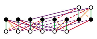
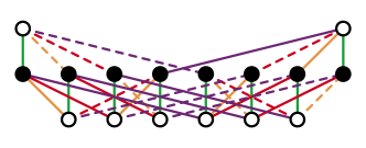
Figure 1: Two four-color inequivalent (6$|$8$|$2) adinkras.

are clearly not isomorphic. One would need to look at sixty-four separate equations to prove this by conventional means. This example leads to the question of how to determine whether two arbitrary adinkra graphs are isomorphic in shape to each other, especially when the graphs themselves may be too complicated to visually inspect. In this paper, we will demonstrate an algorithm which can easily determine shape isomorphisms in a computer friendly manner.

From past investigations, we know simple ways of determining adinkra isomorphisms become increasingly unwieldy for adinkras of increasing complicated structure (see Ref.  [2] for such an example), therefore previous work [3] created an algorithm which could determine isomorphisms for any adinkra. The algorithm is computationally inefficient due to its unnecessarily complicated structure. Therefore, the need for dependable and efficient algorithms that are computationally simple is well motivated.

The new algorithm presented in this work for determining adinkra shape isomorphisms is a generalization of a previously presented algorithm [4] used to consistently describe a set of supersymmetrical equation describing a two dimensional system. We introduced in this work ‘permutation matrices’ which, when multiplied by a super vector of bosons and fermions, $\mathbf{\Phi}\oplus\mathbf{\Psi}$, re-creates the supersymmetrical equations (where the elements in $\mathbf{\Phi}$ and $\mathbf{\Psi}$ may be each arbitrarily ordered separately).

We then multiply these permutation matrices together to create a ‘total permutation matrix.’ By calculating the eigenvalues of this matrix for any given adinkra and comparing its eigenvalues with the eigenvalues of any other adinkra’s total permutation matrix it turns out to be sufficient to determine if two adinkras possess the same shape. This is analogous lining up the teeth of two keys to determine if they belong to the same lock. If we set all the variables in the permutation matrices to 1 and take the trace, we re-create the “chromocharacters” [5], which can determine whether, by node redefinitions, two adinkras can have the same line dashing [3]. These two properties allow one to determine whether two adinkras are isomorphic.

Our paper is organized as follows. In section 2, we will first introduce the new algorithm, and prove it will always uniquely determine adinkras. In section 3, we will briefly review the previous way of determining if adinkras are isomorphic, while in section 4, we determine the efficacy of this algorithm over the previous one. Lastly, in section 5, we demonstrate the power of the new algorithm, by comparing two sets of adinkras using both the new and previous algorithm.

2 The Isomorphism Algorithm

    We first describe the isomorphism algorithm in the cases of the simplest adinkras (see Ref. [1, 5] for definitions of adinkra graphs), and then show why it can uniquely describe adinkras.
The simplest inequivalent two-color adinkras appear in Fig. # 2.

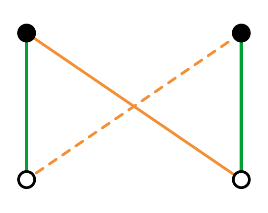
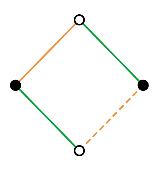
Figure 2: The bow tie (left) and the diamond (right) two-color closed paths.

We use these to create the monochromatic ‘color matrices,’ before we multiply them together, to create the ‘total permutation matrix’ necessary for the algorithm. The diamond adinkra is obtained from the bow tie adinkra by ‘raising’ the bosonic 2-node on the lower right of the bow tie adinkra. The bow tie adinkra (to the left) is also an example of a ‘valise’ adinkra. By definition, these are adinkras where all the bosonic nodes appear at the same height and all the fermionic nodes appear at the same height but where the fermionic height is different from the bosonic height. This naturally leads to a numbering of the nodes lexicographically as shown.

First, to determine adinkra shape, we will ignore line dashing. Line dashing, under well recognized conditions [5], describes the difference between a supermultiplet and its twisted version. This is the reason why we will later on record the adinkra’s chromocharacters, which differentiate line dashing isometries. A point to note is that the matrices associated with these adinkras have the property of possessing a single factor in each row and each column and are thus monomials in the mathematical sense. In addition, these matrices are elements of the permutation group. Upon eliminating the line dashing, the two adinkra graphs above take the forms below in Fig. # 3.

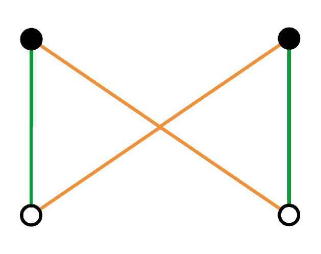
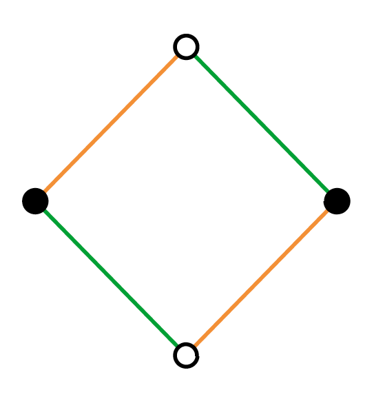
Figure 3: Bow tie and diamond two-color closed paths with line dashing removed.

To form color matrices (each of which is dependent on line color), we first decompose an adinkra into its monochromatic components, as shown in Fig. # 4 for the bow tie, and in Fig. # 5 for the diamond.

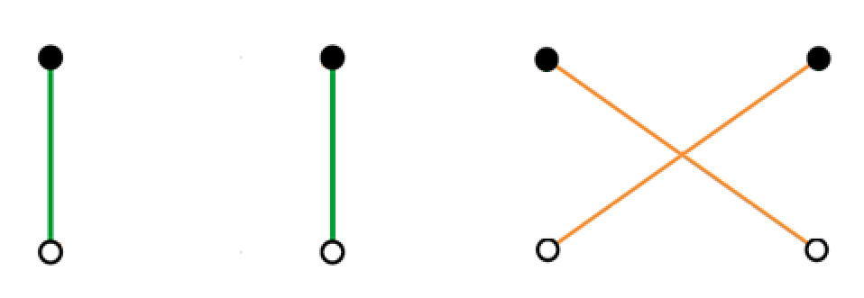
Figure 4: The monochromatic bow tie edges.

In these diagrams, we introduce $N$ distinct parameters ${\beta}{}_{{}_{\rm I}}$, one for each color. We assign a value of ${\beta}{}_{{}_{\rm I}}$ or ${\beta}{}_{{}_{\rm I}}^{-1}$ depending on whether the colored line segment is located above or below the open node attached to it. The ${\beta}{}_{{}_{\rm I}}^{\pm 1}$ assignment is equivalent to multiplying a fermion or boson field, by 1 or $\partial_{\tau}$ in an associated equation within an adinkra, depending on whether the fermion or boson’s associated node is above or below its super partner. For the bosons, we see the correct ${\beta}{}_{{}_{\rm I}}$ assigning in Fig. # 4.

The numerical labels attached to each the nodes allow us to translate each diagram into a matrix. These are the absolute value of the color matrices. We associate each bosonic nodal label with a row entry in a matrix and each fermionic nodal label with a column entry in a matrix. Thus, for the bow tie decomposition, we obtain

$${\|\mathcal{B}}_{1L}\|=\left(\begin{array}[]{cc}\beta_{1}^{-1}&0\\ 0&\beta_{1}^{-1}\\ \end{array}\right)~{}~{}~{},~{}~{}~{}~{}\|\mathcal{B}_{1R}\|=\left(\begin{array}[]{cc}\beta_{1}&0\\ 0&\beta_{1}\\ \end{array}\right)~{}~{}~{},~{}~{}~{}~{}$$ (1)

for the green color permutations and

$$\|\mathcal{B}_{2L}\|=\left(\begin{array}[]{cc}0&\beta_{2}^{-1}\\ \beta_{2}^{-1}&0\\ \end{array}\right)~{}~{}~{},~{}~{}~{}~{}\\ \|\mathcal{B}_{2R}\|=\left(\begin{array}[]{cc}0&\beta_{2}\\ \beta_{2}&0\\ \end{array}\right)~{}~{}~{},$$ (2)

for the yellow line permutations.

As mentioned earlier, we must take into account the line dashing as well, in order to determine whether two adinkras are isomorphic. Therefore, using Fig. # 3, we find that the color matrices (instead of simply the absolute value of them) are:

$${\mathcal{B}}_{1L}=\left(\begin{array}[]{cc}\beta_{1}^{-1}&0\\ 0&\beta_{1}^{-1}\\ \end{array}\right)~{}~{}~{},~{}~{}~{}~{}\mathcal{B}_{1R}=\left(\begin{array}[]{cc}\beta_{1}&0\\ 0&\beta_{1}\\ \end{array}\right)~{}~{}~{},~{}~{}~{}~{}$$ (3)

for the green color permutations and

$$\mathcal{B}_{2L}=\left(\begin{array}[]{cc}0&-\beta_{2}^{-1}\\ \beta_{2}^{-1}&0\\ \end{array}\right)~{}~{}~{},~{}~{}~{}~{}\\ \mathcal{B}_{2R}=\left(\begin{array}[]{cc}0&\beta_{2}\\ -\beta_{2}&0\\ \end{array}\right)~{}~{}~{},$$ (4)

for the yellow line permutations.

We associate 1 and $\partial_{\tau}$ respectively with ${\beta}{}_{{}_{\rm I}}$ and ${\beta}{}_{{}_{\rm I}}^{-1}$. For the green lines in Fig. # 2, we find,

$${\rm D}{}_{{}_{\rm I}}\mathbf{\Phi}=\dot{\imath}\mathcal{B}{}_{{}_{\rm I}R}\mathbf{\Psi}$$ (5)

where $\mathbf{\Phi}$ corresponds to the vector of bosons, and $\mathbf{\Psi}$ corresponds to the vector of fermions. In a similar manner, we have

$${\rm D}{}_{{}_{\rm I}}\mathbf{\Psi}=\mathcal{B}{}_{{}_{\rm I}L}\mathbf{\Phi}$$ (6)

Therefore $\mathbf{\Phi}$ multiplied by $\mathcal{B}_{1R}\mathcal{B}_{2L}$ from the left is equivalent to the operation D₂ D${}_{1}\mathbf{\Phi}$, or similarly equivalent to following the green line and then the yellow line from one boson to another.

Next we can repeat all the steps above but now applied to the diamond adinkra (Fig # 3).

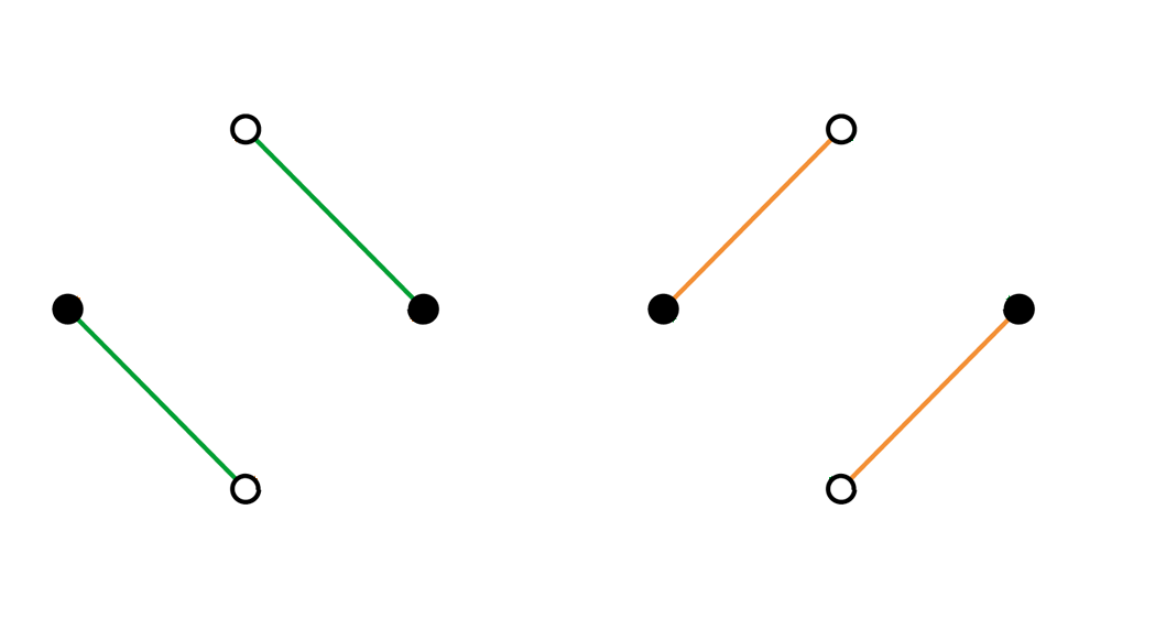
Figure 5: The monochromatic diamond edges.

It can easily be shown that the matrices are

$${{\mathcal{B}}_{1L}=\left(\begin{array}[]{cc}\beta_{1}^{-1}&0\\ 0&\beta_{1}\\ \end{array}\right)~{}~{}~{},~{}~{}~{}~{}\mathcal{B}_{1R}=\left(\begin{array}[]{cc}\beta_{1}&0\\ 0&\beta_{1}^{-1}\\ \end{array}\right)~{}~{}~{},~{}~{}~{}~{}}$$ (7)

for the green line permutations and

$$\mathcal{B}_{2L}=\left(\begin{array}[]{cc}0&-\beta_{2}\\ \beta_{2}^{-1}&0\\ \end{array}\right)~{}~{}~{},~{}~{}~{}~{}\\ \mathcal{B}_{2R}=\left(\begin{array}[]{cc}0&\beta_{2}\\ -\beta_{2}^{-1}&0\\ \end{array}\right)~{}~{}~{},$$ (8)

for the yellow line permutations. Following the logic of the discussion given for the bowtie adinkra that led to (5), an equation of the same form can be obtained for the diamond adinkra. The only difference is that for the diamond the matrix ${\mathcal{B}}_{1L}$ is the one given in (7).

To make path tracing more explicit, let us first define the color dependent block matrix, which permute the super vector $\mathbf{\Phi}\oplus\mathbf{\Psi}$ as defined below. $\mathbf{Definition~{}1:}$Let the matrix $\mathbf{C_{j}}$ be the color block matrix associated with the $j^{th}$ line color. We define

$$\mathbf{C_{j}}\equiv\left(\begin{array}[]{cc}0&\mathbf{\mathcal{B}_{jR}}\\ \mathbf{\mathcal{B}_{jL}}&0\\ \end{array}\right)$$ (9)

where $\mathcal{B}_{jR}$ is the color matrix that permutes bosons to fermions and $\mathcal{B}_{jL}$ is the color matrix the permutes fermions to bosons.

To create what we call an ‘isomorphism matrix’, we can simply multiply all the color matrices from $\mathbf{\mathbf{C_{N}}}$ to $\mathbf{\mathbf{C_{1}}}$ from the left (which is equivalent to following a $N$-distinct color path with the specified color order from every node):

$$\mathcal{B}=\mathbf{C_{N}}\mathbf{C_{N-1}}...\mathbf{C_{1}}$$ (10)

Because every path can be covered by strictly looking at the $N$-distinct color paths from boson or fermion nodes alone, we claim that we can uniquely describe the adinkra up to line dashing by finding the eigenvalues in the matrix $\mathcal{B}_{N(R/L)}...\mathcal{B}_{1R}$ where the first matrix is $\mathcal{B}_{NR}$ if there is an odd number of lines, and $\mathcal{B}_{NL}$ for an even number of lines.

If we were to inspect the eigenvalues of $\|\mathcal{B}_{1R}\mathcal{B}_{2L}\|$ in the diamond adinkra for example, we would find the eigenvalues are ${\beta}_{1}{\beta}_{2}$ and ${\beta}_{1}^{-1}{\beta}_{2}^{-1}$ while the bow tie adinkra has the eigenvalues $\pm{\beta}_{2}{\beta}_{1}^{-1}$, where the $\pm$ sign reflects the degenerate paths each boson takes in the bow tie. These two adinkras create distinct eigenvalues which agrees nicely with our statement above.

In general, finding the absolute value of the eivenvalues will determine adinkra shape, while setting ${\beta}_{1},...,{\beta}_{N}$ to 1, and taking the trace of $\mathcal{B}_{N(R/L)}...\mathcal{B}_{1R}$ will determine the chromocharacters and hence the dashing isometry. These two values is all one needs to determine whether two adinkras are isometric. For the adinkras in Fig. # 4, we find the chromocharacters are 0, by setting ${\beta}_{1}$ and ${\beta}_{2}$ to 1.

Furthermore, we claim that relabeling nodes and re-defining the parity of nodes will not effect the absolute value of the eigenvalues (trivially the trace is basis independent). We can understand why by noting that permuting the adinkra nodes is equivalent to multiplying the equivalence matrix, $\mathcal{B}$ by

$$\mathcal{B}~{}~{}~{}\rightarrow~{}~{}~{}\mathcal{B}\left(\begin{array}[]{cc}\mathbf{\mathcal{P}_{1}}&0\\ 0&\mathbf{\mathcal{P}_{2}}\\ \end{array}\right)$$ (11)

where $\mathcal{P}_{i}$ are permutation matrices. Because permutation matrices only move elements of the matrix around, and therefore do not affect eigenvalues, $\mathcal{B}$’s eigenvalues remain the same.

The following theorem will explain why the algorithm always determines whether adinkras are isomorphic.

$$\mathbf{Theorem~{}1}$$

Two adinkras are isomorphic if and only if their associated eigenvalues of
$\|\mathcal{B}_{N(L/R)}\mathcal{B}_{[N-1](R/L)}...\mathcal{B}_{1R}\|$ (or equivalently $\|\mathcal{B}_{N(R/L)}...\mathcal{B}_{1L}\|$) are the same and their chromocharacters are the same.

$\mathbf{Proof:}$

   To prove the first part, we recall each eigenvalue carries information within the matrices $\|\mathcal{B}_{N(L/R)}\mathcal{B}_{[N-1](R/L)}...\mathcal{B}_{1R}\|$ and $\|\mathcal{B}_{N(R/L)}...\mathcal{B}_{1L}\|$ that corresponds to the orientation upward or downward of a each colored line in an $N$-distinct color path. Because an adinkra has no more than one of each color at every node, a $N$-distinct color path that starts from strictly boson or strictly fermion nodes, will never share the same colored lines as another from the same type of node. Also, because every node has every color, every line would be included if we only record $N$-distinct color paths from bosons or fermions.

If this was not the case, then there would exist a line that cannot be reached by an $N$-distinct color path from either type of node. Because every node has every color, however, every line color (besides the line itself) can connect to that ‘un-reachable’ line from two directions. Therefore, there exists a fermion node and boson node that is less than length $N$ away such that, given an arbitrary order of path colors, it will reach the ‘un-reachable’ line in a path of length less than $N$. Therefore, recording $N$-distinct color paths from the boson or fermion nodes will describe the movement of every colored line.

Now, we will prove that the $N$-distinct color paths are the same if and only if the adinkras are the same.

Trivially, if two adinkras are the same, then each $N$-distinct color path is the same. We are therefore left to prove the converse: if every $N$-distinct color path is the same, then the adinkras must be the same. If the adinkras were different, then there would be a $N$-distinct color path between two nodes (of some arbitrary color order) that is not the same between two adinkras. Because all the $N$-distinct color paths include every line, this would imply at least one of the $N$-distinct color paths with the color order $\|\mathbf{C_{N}}\mathbf{C_{N-1}}...\mathbf{C_{1}}\|$ is different, which is not possible.

Lastly, to prove the second part, we recall that setting all the $\beta$ variables to 1 and taking the trace of $\mathcal{B}_{N(L/R)}\mathcal{B}_{[N-1](R/L)}...\mathcal{B}_{1R}$ or $\mathcal{B}_{N(R/L)}...\mathcal{B}_{1L}$ gives us the adinkra’s associated chromocharacter, which determines line dashing isomorphisms.

If two adinkras are the same shape, and have the same dashing isomorphisms, then trivially, they are isomorphic.

$\Box$

To better understand the difference between the old and new algorithm, let us formally introduce the previous way of identifying isomorphism classes of adinkras.

3 A Review of Past Adinkra Equivalence Algorithm

    Here we present the previous algorithm for determining the isomorphic class of a set of SUSY equations via an adinkra (This section was taken from [6]).

Firstly, we organize nodes according to distance from some arbitrary node $v$, and then organize each subset of nodes of a given distance by their lexicographically shortest path to $v$, as shown below.

$\mathbf{Construction}$ $\mathbf{2}$:
Given an adinkra, and the ordered set of colored lines $\{i_{1},i_{2},...i_{\mathcal{N}}\}$, let us choose an arbitrary node, $v$. We define the function $\lambda_{v}:V\rightarrow[2^{\mathcal{N}-k}]$, as follows, where V is the set of adinkra vertices, and $k$ is the number of non-hypercubic lines.

• $\lambda_{v}(v)=1$.

• Order the nearest neighbors of $v$ from 2 to $\mathcal{N}+1$ based on the rank of the colored lines. In general, $\lambda_{v}(i_{n}v)=1+n,1\leq n\leq N$.

• Look at vertices a distance 2 away from $v$, and organize nodes equivalently, then the vertices a distance 3 away, and so on until all nodes are mapped to $[2^{\mathcal{N}-k}]$.

We will next inspect an adinkra with $h$ height assignments, and organize the $[2^{k}]$ set of orbits in an adinkra with a function $\tau$ which assigns the ‘$a^{th}$’ orbit the number ‘$a$’. Next we define $\mu_{g}(h,a)$, which counts the number of nodes at a given height $h$ in the orbit $a$:

$$\mu_{g}(h,a)=|\{v\in V:\text{hgt}(v)=h,\tau(v)=a\}|$$ (12)

where $\text{hgt}(v)$ is the relative height of the node from the bottom row. It can be shown that the certificate set,

$$\text{cert}_{G}(x)=\{(\lambda_{v}(x),\text{hgt}(x),\tau(x)):x\in V\}$$ (13)

can completely determine the isomorphism class of an adinkra [3]. Despite the seeming simplicity, the authors did not demonstrate how to implement this algorithm except by tracing paths with your finger. With large adinkras (e.g. SUGRA $\mathcal{N}=32$ adinkras), there is a great motivation to determine isomorphisms by computer instead of by hand. How, one might ask, do we determine heights and orbits for a given adinkra computationally? More importantly, how can we do this efficiently? The previous paper left these glaring questions unanswered.

This is the motivation behind efficiently distinguish isomorphism classes via color matrices.

4 On the Question of Efficiency

   Given the previous algorithm, we run into a question regarding the relative efficiency of color matrix-based equivalence algorithms.

Although our current algorithm only determines equivalence classes, we can easily use R- and L-matrices to determine cis- and trans adinkras, thus allowing the complete isomorphism class of the adinkra to be determined. Thus, we have an effective algorithm for determining isomorphism, but a quick look tells us we need a relatively enormous amount of memory to determine isomorphisms compared to the previous algorithm.

Recall that we need a color matrix for every color with elements associated with every node. This gives $\cal N$ numbers for every node up to the value $\cal N$. Furthermore we need to denote $\pm$ signs for every R (L-matrices are transposes so they do not need to be recorded). This gives us $\mathcal{N}\text{log}_{2}(\mathcal{N})+\mathcal{N}/2$ bits to be recorded per node, or

$$2^{\mathcal{N}-k}\left[\mathcal{N}(\frac{1}{2}+\text{log}_{2}(\mathcal{N}))\right]$$ (14)

bits total. In comparison, The previous algorithm needed

$$2^{\mathcal{N}-k}\left[\mathcal{N}+\text{log}_{2}(\mathcal{N})\right]$$ (15)

bits. Despite this disadvantage, the previous algorithm is impractical because there is no known computer-friendly way of determining orbits and levels [6]. More importantly, computer programs like Matlab are made for matrices, which reduces extra coding, and matlab code can be added onto the GPU, allowing matrices to be created and computed with orders of magnitude greater efficiency. It is because of these two distinct advantages that the algorithm has some practical uses.

5 Comparing Two Sets of Distinct Adinkras Using The Different Equivalence Algorithms

     Now we will apply this algorithm to two known adinkra sets, each of which have fundamentally distinct equations. In addition, we will show that each set of adinkras are distinct using the algorithm in [3], in order to demonstrate our algorithms superiority at determining adinkra equivalence with greater computational efficiency.

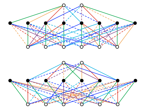
Figure 6: Our first set of adinkras being tested

In the adinkras, the following conventions are utilized: ‘1’ is green, ‘2’ is yellow, ‘3’ is red, ‘4’ is purple, ‘5’ is light blue and ‘6’ is dark blue. Because chromocharacters have been demonstrated to differentiate line dashing isomorphisms, we will simply look at the difference in adinkra shape with our algorithm. Here, both adinkras have the same dashing and hence have the same chromocharacters. For both sets of adinkras, we will list the color matrices $\|\mathbf{C_{1}}\|$ through $\|\mathbf{C_{6}}\|$, in Appendix A and Appendix B respectively, and compute the eigenvalues of $\|\mathcal{B}_{6L}...\mathcal{B}_{1R}\|$ and $\|\mathcal{B}_{6R}...\mathcal{B}_{1L}\|$ below to demonstrate that the eigenvalues of two former matrices can adequately determine adinkra uniqueness, without having to resort to taking the eigenvalues of the entire $\mathcal{B}$ matrix.

For the first adinkra in Figure 6, The eigenvalues for $\|\mathcal{B}_{6L}...\mathcal{B}_{1R}\|$ are

$$\pm 1\,(\text{2x degenerate})~{}~{},~{}~{}\pm{\beta}_{2}{\beta}_{4}{\beta}_{6}{\beta}_{1}^{-1}{\beta}_{3}^{-1}{\beta}_{5}^{-1}\,(\text{2x degenerate})~{}~{}~{},$$ (16)

and the eigenvalues for $\|\mathcal{B}_{6R}...\mathcal{B}_{1L}\|$ are

$$\pm\beta_{1}{\beta}_{2}^{-1}\,(\text{2x degenerate})~{}~{},~{}~{}\pm\beta_{3}\beta_{5}\beta_{4}^{-1}\beta_{6}^{-1}\,(\text{2x degenerate})~{}~{}~{}.$$ (17)

For the second adinkra, the eigenvalues for $\|\mathcal{B}_{6L}...\mathcal{B}_{1R}\|$ are

$$\pm\beta_{2}\beta_{4}\beta_{6}\beta_{1}^{-1}\beta_{3}^{-1}\beta_{5}^{-1}(\text{3x degenerate})~{}~{},~{}~{}\pm\beta_{1}\beta_{3}\beta_{5}\beta_{2}^{-1}\beta_{4}^{-1}\beta_{6}^{-1}~{}~{},$$ (18)

and the eigenvalues for $\|\mathcal{B}_{6R}...\mathcal{B}_{1L}\|$ in the second adinkra are

 

$${{}\pm\beta_{1}\beta_{3}\beta_{5}\beta_{2}^{-1}\beta_{4}^{-1}\beta_{6}^{-1}~{}~{},~{}~{}\pm\beta_{2}\beta_{3}\beta_{5}\beta_{1}^{-1}\beta_{4}^{-1}\beta_{6}^{-1}~{}~{}~{},}$$

  (19)

We note that the sets of eigenvalues are distinct from the previous adinkra.

The previous algorithm used the following set

$$cert_{G}(v)=\{(\lambda_{v}(x),hgt(x),\tau(x)):x\in V\}$$ (20)

to determine equivalence, where $\lambda_{v}(x)$ organizes the nodes to determine if two adinkras are the same ignoring dashing or automorhpisms. $hgt(x)$ determines the absolute height of the node (e.g. 2 rows from the bottom row). $\tau(x)$ is used to determine the orbits of an adinkra.

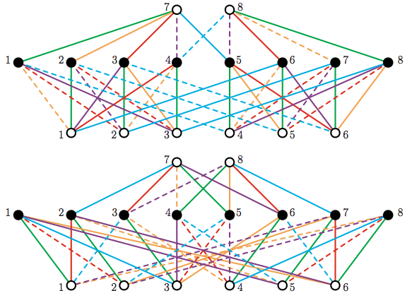
Figure 7: The second set of adinkras being tested

Our next adinkra pair in Fig. # 7 is the same as the previous except without the dark blue lines, hence the color matrices $C_{J}$ are the same except there is no $\mathbf{C_{6}}$.

For the first adinkra, the eigenvalues of $\|\mathcal{B}_{5R}...\mathcal{B}_{1R}\|$ are

$\beta_{1}^{1/3}\beta_{3}^{1/3}\beta_{5}^{1/3}\beta_{2}^{-1}\beta_{4}^{-1/3},\$$-(-1)^{1/3}\beta_{1}^{1/3}\beta_{3}^{1/3}\beta_{5}^{1/3}\beta_{2}^{-1}\beta_{4}^{-1/3},\$$(-1)^{2/3}\beta_{1}^{1/3}\beta_{3}^{1/3}\beta_{5}^{1/3}\beta_{2}^{-1}\beta_{4}^{-1/3},\$$\beta_{1}^{1/5}\beta_{3}^{3/5}\beta_{5}^{3/5}\beta_{2}^{-1/5}\beta_{4}^{-3/5},\$$-(-1)^{1/5}\beta_{1}^{1/5}\beta_{3}^{3/5}\beta_{5}^{3/5}\beta_{2}^{-1/5}\beta_{4}^{-3/5},\$$(-1)^{2/5}\beta_{1}^{1/5}\beta_{3}^{3/5}\beta_{5}^{3/5}\beta_{2}^{-1/5}\beta_{4}^{-3/5},\$$-(-1)^{3/5}\beta_{1}^{1/5}\beta_{3}^{3/5}\beta_{5}^{3/5}\beta_{2}^{-1/5}\beta_{4}^{-3/5},\$

$$(-1)^{4/5}\beta_{1}^{1/5}\beta_{3}^{3/5}\beta_{5}^{3/5}\beta_{2}^{-1/5}\beta_{4}^{-3/5}$$ (21)

The eigenvalues of $\|\mathcal{B}_{5L}...\mathcal{B}_{1L}\|$ are

$\beta_{2}^{1/5}\beta_{4}^{3/5}\beta_{1}^{-3/5}\beta_{3}^{-1/5}\beta_{5}^{-3/5},\$$-(-1)^{1/5}\beta_{2}^{1/5}\beta_{4}^{3/5}\beta_{1}^{-3/5}\beta_{3}^{-1/5}\beta_{5}^{-3/5},\$ $(-1)^{2/5}\beta_{2}^{1/5}\beta_{4}^{3/5}\beta_{1}^{-3/5}\beta_{3}^{-1/5}\beta_{5}^{-3/5},\$$-(-1)^{3/5}\beta_{2}^{1/5}\beta_{4}^{3/5}\beta_{1}^{-3/5}\beta_{3}^{-1/5}\beta_{5}^{-3/5},\$$(-1)^{4/5}\beta_{2}^{1/5}\beta_{4}^{3/5}\beta_{1}^{-3/5}\beta_{3}^{-1/5}\beta_{5}^{-3/5},\$$\beta_{2}\beta_{4}^{1/3}\beta_{1}^{-1/3}\beta_{3}^{-1}\beta_{5}^{-1/3},\$ $-(-1)^{1/3}\beta_{2}\beta_{4}^{1/3}\beta_{1}^{-1/3}\beta_{3}^{-1}\beta_{5}^{-1/3},\$

$$(-1)^{2/3}\beta_{2}\beta_{4}^{1/3}\beta_{1}^{-1/3}\beta_{3}^{-1}\beta_{5}^{-1/3}$$ (22)

In comparison, for the second adinkra, the eigenvalues of $\|\mathcal{B}_{5R}...\mathcal{B}_{1R}\|$ are

$\beta_{1}^{1/5}\beta_{3}\beta_{5}^{1/5}\beta_{2}^{-1/5}\beta_{4}^{-1},\$$-(-1)^{1/5}\beta_{1}^{1/5}\beta_{3}\beta_{5}^{1/5}\beta_{2}^{-1/5}\beta_{4}^{-1},\$$(-1)^{2/5}\beta_{1}^{1/5}\beta_{3}\beta_{5}^{1/5}\beta_{2}^{-1/5}\beta_{4}^{-1},\$$-(-1)^{3/5}\beta_{1}^{1/5}\beta_{3}\beta_{5}^{1/5}\beta_{2}^{-1/5}\beta_{4}^{-1},\$$(-1)^{4/5}\beta_{1}^{1/5}\beta_{3}\beta_{5}^{1/5}\beta_{2}^{-1/5}\beta_{4}^{-1},\$$-\beta_{1}\beta_{3}\beta_{5}\beta_{2}^{-1}\beta_{4}^{-1},\$

$$\pm\beta_{1}\beta_{5}\beta_{2}^{-1}$$ (23)

The eigenvalues for $\|\mathcal{B}_{5L}...\mathcal{B}_{1L}\|$ are

$\beta_{2}^{1/5}\beta_{4}\beta_{1}^{-1/5}\beta_{3}^{-1}\beta_{5}^{-1/5},\$$-(-1)^{1/5}\beta_{2}^{1/5}\beta_{4}\beta_{1}^{-1/5}\beta_{3}^{-1}\beta_{5}^{-1/5},\$$(-1)^{2/5}\beta_{2}^{1/5}\beta_{4}\beta_{1}^{-1/5}\beta_{3}^{-1}\beta_{5}^{-1/5},\$$-(-1)^{3/5}\beta_{2}^{1/5}\beta_{4}\beta_{1}^{-1/5}\beta_{3}^{-1}\beta_{5}^{-1/5},\$$(-1)^{4/5}\beta_{2}^{1/5}\beta_{4}\beta_{1}^{-1/5}\beta_{3}^{-1}\beta_{5}^{-1/5},\$$-\beta_{2}\beta_{4}\beta_{1}^{-1}\beta_{3}^{-1}\beta_{5}^{-1},\$

$$\beta_{2}\beta_{4}\beta_{1}^{-1}\beta_{3}^{-1}\beta_{5}^{-1}(\text{3x degenerate})$$ (24)

Using the old algorithm, we find that although $\lambda(x)$ is the same, we find that

$~{}~{}~{}~{}~{}~{}~{}~{}~{}~{}~{}~{}\mu_{G}(3,1)=1~{}~{}~{}~{}~{}~{}~{}~{}~{}~{}~{}~{}~{}~{}~{}~{}~{}~{}~{}~{}~{}~{}~{}~{}~{}~{}~{}~{}~{}~{}~{}\mu_{H}(3,1)=2\newline ~{}~{}~{}~{}~{}~{}~{}~{}~{}~{}~{}~{}~{}~{}~{}~{}~{}\mu_{G}(3,2)=1~{}~{}~{}~{}~{}~{}~{}~{}~{}~{}~{}~{}~{}~{}~{}~{}~{}~{}~{}~{}~{}~{}~{}~{}~{}~{}~{}~{}~{}~{}~{}~{}\mu_{H}(3,2)=0\newline ~{}~{}~{}~{}~{}~{}~{}~{}~{}~{}~{}~{}~{}~{}~{}~{}~{}\mu_{G}(2,1)=\mu_{G}(2,2)=4~{}~{}~{}~{}~{}~{}~{}~{}~{}~{}~{}~{}~{}~{}~{}~{}~{}~{}\mu_{H}(2,1)=\mu_{H}(2,2)=4\newline ~{}~{}~{}~{}~{}~{}~{}~{}~{}~{}~{}~{}~{}~{}~{}~{}~{}\mu_{G}(1,1)=3~{}~{}~{}~{}~{}~{}~{}~{}~{}~{}~{}~{}~{}~{}~{}~{}~{}~{}~{}~{}~{}~{}~{}~{}~{}~{}~{}~{}~{}~{}~{}~{}\mu_{H}(1,1)=2\newline ~{}~{}~{}~{}~{}~{}~{}~{}~{}~{}~{}~{}~{}~{}~{}~{}~{}\mu_{G}(1,2)=3~{}~{}~{}~{}~{}~{}~{}~{}~{}~{}~{}~{}~{}~{}~{}~{}~{}~{}~{}~{}~{}~{}~{}~{}~{}~{}~{}~{}~{}~{}~{}~{}\mu_{H}(1,2)=4$
and clearly the the automorphisms are not the same. This, again, took significantly longer to determine both because nodes had to be organized, and needs height determination to generally determine the in-equivalence of two adinkras, which is again not necessary for our current algorithm

6 Conclusion

     In this paper, we presented a new algorithm to determine whether two adinkras are isomorphic, using the trace of of $\mathcal{B}_{N(R/L)}...\mathcal{B}_{1R}$, setting all variables to 1, and by using the eigenvalues of the absolute value of the above matrix. These eigenvalues correspond to $N$-length unique color paths from bosons (if $\mathcal{B}_{NR}$), or fermions (if $\mathcal{B}_{NL}$). It is clear that not only is the algorithm efficient, but can disregard the order of the node labels. Furthermore, despite the comparative inefficiency of this algorithm compared to [3] the algorithm is much more computer friendly, and can be computed with parallel processors saving even more time in the process.

  

   
     “A good picture is equivalent to a good deed. ”   

        – Vincent Van Gogh
   

Acknowledgments

This research was supported in part by the endowment of the John S. Toll Professorship, the University of Maryland Center for String & Particle Theory, National Science Foundation Grant PHY-09-68854. Additionally KB acknowledges participation in 2012 SSTPRS (Student Summer Theoretical Physics Research Session). Adinkras were drawn with Adinkramat $\copyright$ 2008 by G. Landweber.

7 Appendix A

The color matrices, $C_{J}$, for the first adinkra in Fig. # 6 are listed below. For all the adinkras in Appendix B and C, I used the convention: “1” is green, “2” is yellow, “3” is red, “4” is purple, “5” is light blue and “6” is dark blue. The color matrices for the first adinkra in Fig. # 7 are the same, except without the final matrix, $\mathbf{C_{6}}$.

$$\vbox{\hbox{\hss \begin{picture}(-20.0,0.0)\put(-77.0,-88.0){\includegraphics[width=433.62pt]{figures/Adnk1C1}} \end{picture}\hss}}.$$

$$\vbox{\hbox{\hss \begin{picture}(-20.0,0.0)\put(-77.0,-88.0){\includegraphics[width=433.62pt]{figures/Adnk1C2}} \end{picture}\hss}}.$$

$$\vbox{\hbox{\hss \begin{picture}(-20.0,0.0)\put(-77.0,-88.0){\includegraphics[width=433.62pt]{figures/Adnk1C3}} \end{picture}\hss}}.$$

$$\vbox{\hbox{\hss \begin{picture}(-20.0,0.0)\put(-77.0,-88.0){\includegraphics[width=433.62pt]{figures/Adnk1C4}} \end{picture}\hss}}.$$

$$\vbox{\hbox{\hss \begin{picture}(-20.0,0.0)\put(-77.0,-88.0){\includegraphics[width=433.62pt]{figures/Adnk1C5}} \end{picture}\hss}}.$$

$$\vbox{\hbox{\hss \begin{picture}(-20.0,0.0)\put(-77.0,-88.0){\includegraphics[width=433.62pt]{figures/Adnk1C6}} \end{picture}\hss}}.$$

8 Appendix B

The color matrices, $C_{J}$, for the second adinkra in Fig. # 6 are listed below. For all the adinkras in Appendix B and C, I used the convention: “1” is green, “2” is yellow, “3” is red, “4” is purple, “5” is light blue and “6” is dark blue. The color matrices for the second adinkra in Fig. # 7 are the same, except without the final matrix, $\mathbf{C_{6}}$.

$$\vbox{\hbox{\hss \begin{picture}(-20.0,0.0)\put(-77.0,-48.0){\includegraphics[width=433.62pt]{figures/Adnk2C1}} \end{picture}\hss}}.$$

$$\vbox{\hbox{\hss \begin{picture}(-20.0,0.0)\put(-77.0,-48.0){\includegraphics[width=433.62pt]{figures/Adnk2C2}} \end{picture}\hss}}.$$

$$\vbox{\hbox{\hss \begin{picture}(-20.0,0.0)\put(-77.0,-88.0){\includegraphics[width=433.62pt]{figures/Adnk2C3}} \end{picture}\hss}}.$$

$$\vbox{\hbox{\hss \begin{picture}(-20.0,0.0)\put(-77.0,-88.0){\includegraphics[width=433.62pt]{figures/Adnk2C4}} \end{picture}\hss}}.$$

$$\vbox{\hbox{\hss \begin{picture}(-20.0,0.0)\put(-77.0,-88.0){\includegraphics[width=433.62pt]{figures/Adnk2C5}} \end{picture}\hss}}.$$

$$\vbox{\hbox{\hss \begin{picture}(-20.0,0.0)\put(-77.0,-88.0){\includegraphics[width=433.62pt]{figures/Adnk2C6}} \end{picture}\hss}}.$$

References

- [1] M. Faux, and S. J. Gates, Jr., “Adinkras: A Graphical Technology for Supersymmetric Representation Theory, Phys. Rev. D71 (2005) 065002, arXiv:0408004.
- [2] C. F. Doran, M. G. Faux, S. J. Gates, Jr., T. Hubsch, K. M. Iga, G. D. Landweber, “A Counter-Example to a Putative Classification of 1-Dimensional, N-extended Supermultiplets,” Adv. Studies Theor. Phys., Vol. 2, 2008, no. 3, 99, 2008, arXiv:hep-th/0611060v2.
- [3] B. L. Douglas, S. J. Gates, Jr., J. B. Wang, “Automorphism Properties of Adinkras,” Univ. of Maryland Preprint # UMDEPP-10-014, Sep 2010, arXiv:1009.1449 [hep-th], unpublished.
- [4] Keith Burghardt, S. J. Gates, Jr., “A Computer Algorithm For Engineering Off-Shell Multiplets With Four Supercharges On The World Sheet” Univ. of Maryland Preprint # UMDEPP-012-016, October 2012, arXiv:1209.5020 [hep-th].
- [5] S. J. Gates, Jr., J. Gonzales, B. MacGregor, J. Parker, R. Polo-Sherk, V. G. J. Rodgers, and L. Wassink, “4D, N = 1 supersymmetry genomics (I),” JHEP 12 (2009) 008, arXiv:0902.3830 [hep-th].
- [6] Keith Burghardt, “Less is More,” Univ. of Maryland preprint PP-012-017, in preparation.