Keplerian Dynamics on the Heisenberg Group and Elsewhere

Abstract.

Posing Kepler’s problem of motion around a fixed “sun” requires the geometric mechanician to choose a metric and a Laplacian. The metric provides the kinetic energy. The fundamental solution to the Laplacian (with delta source at the “sun”) provides the potential energy. Posing Kepler’s three laws (with input from Galileo) requires symmetry conditions. The metric space must be homogeneous, isotropic, and admit dilations. Any Riemannian manifold enjoying these three symmetry properties is Euclidean. So if we want a semblance of Kepler’s three laws to hold but also want to leave the Euclidean realm, we are forced out of the realm of Riemannian geometries. The Heisenberg group (a subRiemannian geometry) and lattices provide the simplest examples of metric spaces enjoying a semblance of all three of the Keplerian symmetries. We report success in posing, and solving, the Kepler problem on the Heisenberg group. We report failures in posing the Kepler problem on the rank two lattice and partial success in solving the problem on the integers. We pose a number of questions.

1. Introduction

Newton formulated and solved what we call today “Kepler’s problem” – the problem whose negative energy solutions are Keplerian ellipses. The essential backdrop to the problem is Euclidean three-space and its group of isometries and scalings. Can we pose Kepler’s problem on an arbitrary metric space? What properties must the space have if Kepler’s three laws, or ghosts of these laws, are to hold?

In ‘Foundations of Mechanics’ ([1]), Abraham and Marsden formulate classical mechanics as dynamical systems on the tangent bundle or cotangent bundle of a Riemannian manifold, which they call “natural mechanical systems”. The Riemannian metric defines the kinetic energy. One must choose a potential energy. In order to formulate Kepler’s problem on our manifold, we take this potential to be the fundamental solution to the Laplacian. We choose a point on the manifold to be our “sun,” which is the delta function source of the fundamental solution. Following Galileo we assume that the choice of location of the sun does not matter: that is, we will assume that our space is homogeneous.

The mildest Riemannian departures from Euclidean space are the spaces of constant curvature: the sphere and hyperbolic space. About a century and a half before ‘Foundations,’ Lobachevksy ([11]), one of the founders of hyperbolic geometry, posed the Kepler problem as a “natural mechanical system” on hyperbolic space. Later, Serret ([15]) posed the Kepler problem on the sphere. We are grateful to F. Diacu for these references and his survey [6]. Kepler’s 1st and 2nd laws hold in each of the three constant curvature geometries: hyperbolic space, the 3-sphere, and the original flat Euclidean space. But Kepler’s 3rd law fails for these non-flat geometries for the simple reason that they admit no continuous scaling symmetries, or “dilations.”

We argue that in order to even formulate Kepler’s third law our metric space must admit dilations. But if a space admits dilations, and is not Euclidean, then it cannot even be Riemannian! (We sketch the proof of this fact below.) The non-Euclidean spaces which admit dilations are subRiemannian: they are the Carnot groups. The simplest Carnot group is the Heisenberg group.

This observation brings us to our main problem: pose and solve the the Kepler problem on the Heisenberg group. We will pose it. We will not fully solve it. We will show that all periodic solutions to the Kepler problem on the Heisenberg group must lie on the zero energy surface, and that the problem is integrable when restricted to this zero energy surface. Such solutions are described in Figures 2 and 4. A modified version of Kepler’s third law holds for the periodic solutions.

To write down the Kepler-Heisenberg problem we must have an explicit expression for the potential: it is the fundamental solution for the subLaplacian on the Heisenberg group. Luckily, Folland ([5]) found such an expression in 1970.

We will also attempt to pose and solve Kepler’s problem on some lattices. Lattices almost admit dilations: we can scale by positive integer scaling factors, but we cannot invert these scaling factors. The integers form the simplest lattice. We will pose and solve a Kepler problem on the integers. Our ‘solutions’ are of a high school nature. (We apologize in advance if our treatment here embarrasses readers with any skill in numerical methods and discretization.) These solutions are indicated in Figure 5.

We then try to pose and solve the Kepler problem on the integer lattice in the plane where we run into fundamental problems which lead us to believe that the very definition of a discrete dynamical system is not yet well formulated. The heart of this problem is that the differences of values of the lattice potential – that being the fundamental solution of the lattice Laplacian – are irrational.

Dedication and Acknowledgements. This article is dedicated to the memory of Jerry and in thanks for all his inspiration. We would also like to thank the GMC group, in particular, David Martín de Diego, Juan Carlos Marrero, and Edith Padron for inviting us to the summer school in 2011 outside of Madrid. The formulation of the Kepler-Heisenberg problem was inspired by talking with many of the participants at that summer school.

2. Kepler’s 3 laws in a metric space.

Let’s recall Kepler’s three laws for the motion of planets around the sun.

K1. Planets travel on ellipses with one focus the sun.

K2. Equal areas are swept out in equal times. This law is equivalent to the conservation of the planet’s angular momentum about the sun.

K3. Period-Size: The period $T$ of an orbit and its size $a$ (semi-major axis) are related by a universal monomial relation $a^{3}=CT^{2}$.

The Keplerian planet moves in a Euclidean space. Do Kepler’s laws even make sense on a general metric space? If not, what restrictions must we impose on the metric space in order to make sense of a particular law? We discuss what is required of our metric space in order to formulate the corresponding law.

K1. We can define an “ellipsoid” for any metric space $X$. Fix two foci $S,F\in X$ and a positive number $2a$. Consider the locus of points $x\in X$ for which $d(S,x)+d(x,F)=2a$. If this locus is to be a curve then the metric space must be two-dimensional, for example, a smooth surface. K1 requires then that $X$ is a two-dimensional, or that its Keplerian dynamics can be reduced to two-dimensions. Kepler’s problem has been posed and solved satisfactorily on the two-sphere and on the hyperbolic plane as described in the introduction. Its solutions satisfy K1.

K2 is equivalent to conservation of angular momentum. Angular momentum is conserved if the kinetic and potential energies in Newton’s formulation of the Kepler problem are invariant under rotations about the sun. This requires isotropicness: all directions in the metric space are the same, at least through the sun. The two-sphere and the hyperbolic plane enjoy rotational symmetry and hence K2.

K3 is a scaling law. It is an immediate consequence of the fact that the Newtonian potential $V(x)=c/|x|$ is homogeneous of degree $-1$. This homogeneity implies the space-time symmetry $x,t\mapsto\lambda x,\lambda^{3/2}t$, which is to say: if $x(t)$ solves Kepler’s equation then so does $\lambda x(\lambda^{-3/2}t)$. From one periodic solution $x(t)$ we generate a one-parameter family $x_{\lambda}$. The energy-period relation in K3 for this family follows from the scaling symmetry

2.0.1. Kepler’s third law for homogeneous potentials in Euclidean space.

Any homogeneous potential $V$ on a Euclidean space enjoys a version of K3. Homogeneity is a scaling symmetry: $x\mapsto\lambda x\implies V(x)\mapsto V(\lambda x)=\lambda^{-\alpha}V(x)$. We try to extend the symmetry to time and velocities by a power law ansatz: $(x,t,v)\mapsto(\lambda x,\lambda^{\beta}t,\lambda^{-\nu}v)$. Balancing the resulting scalings of potential and kinetic energies implies that $\nu=\alpha/2$. The requirement $v=dx/dt$ yields $\beta=1+(\alpha/2)$. We are led to the extended scalings

$$(x,t,v)\mapsto(\lambda x,\lambda^{1+\alpha/2}t,\lambda^{-\alpha/2}v).$$

In terms of curves $\gamma(t)$, which are maps from $t$ to $x$-space, the scaling operation is

$$\gamma(t)\mapsto\gamma_{\lambda}(t)=\lambda\gamma(\lambda^{-(1+\alpha/2)}t).$$

One verifies that if $\gamma$ satisfies Newton’s equation $\ddot{\gamma}=-\nabla V(\gamma)$ then so does $\gamma_{\lambda}$. (Use that $\nabla V$ is homogeneous of degree $-\alpha-1$.) The scaling symmetry thus takes solutions of energy $H$ to solutions of energy $\lambda^{-\alpha}H$. Now if $\gamma$ is periodic of period $T$ and with typical size $a$, then $\gamma_{\lambda}$ is periodic of period $\lambda^{\beta}T=\lambda^{1+\alpha/2}T$ and typical size $\lambda a$. We thus arrive at our modified K3: $T^{2}=Ca^{2+\alpha}$.

2.0.2. Dilations

To have an analogue of K3, our metric space must, like Euclidean space, admit dilations.

Definition 1.

A dilation of the metric space $(X,d)$ with center $S\in X$ and dilation factor $\lambda$ is a map $\delta_{\lambda}:X\to X$ which fixes $S$ and satisfies $d(\delta_{\lambda}x,\delta_{\lambda}y)=\lambda d(x,y)$ for all $x,y\in X$. We say that the metric space $X$ admits dilations if there is a dilation of $X$ with dilation factor $\lambda$ for each $\lambda>0$.

Spherical and hyperbolic metrics admit no dilations. K3 fails for both.

3. Keplerian symmetries.

We will restrict ourselves to metric spaces $X$ which

$$\bullet\text{are homogeneous}$$ (1)

$$\bullet\text{are isotropic}$$ (2)

$$\bullet\text{admit dilations.}$$ (3)

We will call these three properties the Keplerian symmetry assumptions.

Historical Motivation. Newton’s biggest victory was probably his derivation of Kepler’s laws K1,K2, K3, from more basic laws: Galilean invariance, his equation $F=ma$, and the specific choice of force $F$ as ‘$1/r^{2}$.’ From these laws he derived what we today call Kepler’s differential equation $\ddot{q}=-q/|q|^{3}$ and thence K1-3. A subset of the Galilean group is the group of spatial isometries and this relates to homogeneity and isotropicness. Dilations, as discussed above, are included so as to get a version of Kepler’s third law.

We recall the formal definition homogeneity and isotropicness. Let $Isom(X)$ denotes the group of isometries of $X$. Homogeneity asserts that $Isom(X)$ acts transitively on $X$. Isotropicness asserts that $Isom(X)$ acts transitively on the space of directions through any point $S\in X$. The sphere and the hyperbolic plane are homogeneous and isotropic, but they do not admit dilations.

Proposition 1.

If a Riemannian manifold is homogeneous and admits dilations then it is a Euclidean space.

Proof [sketch]. See Gromov [9], prop. 3.15. Gromov defines the metric tangent cone $T_{p}X$ of any metric space at any point $p\in X$ as the pointed limit $(X,\lambda d)$ as $\lambda\to\infty$. This limit need not always exist, but it does exist for Riemannian manifolds and equals the usual tangent plane, with its induced Euclidean metric. If the metric $d$ admits a dilation with scale factor $\lambda$ then $(X,d)$ is isometric to $(X,\lambda d)$. Letting $\lambda\to\infty$ we see that such an $X$ is isometric to its metric tangent cone $T_{p}X$ for all $p$. QED

Consequently, if we insist on satisfying all three Keplerian symmetries (1)-(3) while also leaving the realm of Euclidean spaces, we must also leave the world of Riemannian manifolds! The simplest non-Euclidean metric space satisfying (1)-(3) is the Heisenberg group with its subRiemannian metric.

4. Kepler’s problem and the Laplacian

Before formulating the Kepler-Heisenberg problem, we look into how the standard Kepler problem fits within the framework of “natural mechanical systems” and thus how it generalizes to general Riemannian manifolds. This background will yield a straightforward way to place the Kepler problem in the Heisenberg context.

The Hamiltonian for the standard Kepler problem on $\mathbb{R}^{3}$ is

$$H=\frac{1}{2}(p_{x}^{2}+p_{y}^{2}+p_{z}^{2})-\frac{\alpha}{r},$$

where $r=\sqrt{x^{2}+y^{2}+z^{2}}$ and $\alpha>0.$ Why the $1/r$ potential? Perhaps the best answer is that $U=\frac{1}{4\pi r}$ is the fundamental solution for the Laplacian $\Delta$ on (Euclidean!) $\mathbb{R}^{3}$, i.e. the solution to $\Delta U=-\delta_{0}$. (See [3] and references therein.) The choice of sign convention is due to the positivity of the operator $-\Delta$.

The kinetic term in $H$ is the principal symbol of the Laplacian, so we can write

$$H(q,p)=\frac{1}{2}\sigma_{\Delta}-\alpha\Delta^{-1}_{q}$$ (*)

where $\sigma_{L}$ denotes the principal symbol of $L$, and $\Delta^{-1}(q)=K(q,0),$ where $K(x,y)=U(x-y)$ is the Green’s function for the Laplacian (and where $\alpha=\frac{1}{4\pi}$). This reformulation suggests that we can pose ‘Kepler problem’ as a Hamiltonian system on any ‘space’ $X$ with a ‘Laplacian’ $\Delta$.

This prescription (*) for $H$ leaves us with a number of puzzles.

Problems. What is the cotangent bundle of an arbitrary ‘space’ $X$? Assuming we make sense of $H$ as a function on the cotangent bundle of $X$, then what are Hamilton’s equations on $T^{*}X$? Can we ever compute the fundamental solution $\Delta^{-1}_{q}$ of our Laplacian?

All these questions have answers in the Riemannian case. The principal symbol has the coordinate expression

$$\sigma_{\Delta}(p)=\Sigma g^{ij}(q)p_{i}p_{j}$$

– it is the standard cometric of kinetic energy. The fundamental solution of the Laplacian has been explicitly computed for hyperbolic $n$-space, so we have a hyperbolic Kepler problem.

If $X$ is a compact manifold without boundary, then the fundamental solution $\Delta_{q}^{-1}$ does not exist for topological reasons. For example, we cannot have a single gravitational source on the sphere. There must be an opposing sink elsewhere on the sphere. To formulate the Kepler problem on the sphere, one places the sink antipodally to the source. See [6] or [15] for a precise formulation.

5. Kepler’s Problem on the Heisenberg Group!

5.1. Heisenberg Geometry

Consider $\mathbb{R}^{3}$ with standard $x,y,z$ coordinates, endowed with the two vector fields

$$X={{\partial}\over{\partial x}}-\frac{1}{2}y{{\partial}\over{\partial z}}\qquad Y={{\partial}\over{\partial y}}+\frac{1}{2}x{{\partial}\over{\partial z}}.$$

Then $X,Y$ span the canonical contact distribution $D$ on $\mathbb{R}^{3}$ with induced Lebesgue volume form. Curves are called horizontal if they are tangent to $D$. Declaring $X,Y$ orthonormal defines the standard subRiemannian structure on the Heisenberg group and yields the Carnot-Carathéodory metric $ds^{2}_{\mathbb{H}}=dx^{2}+dy^{2}$. Geodesics are qualitatively helices: lifts of circles and lines in the $xy$-plane. The horizontal constraint implies that the $z$-coordinate of a curve grows like the area traced out by the projection of the curve to the $xy$-plane. See Figure 1 and Chapter 1 of [14].

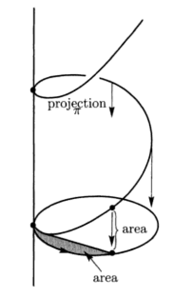
Figure 1. A Heisenberg geodesic

The Heisenberg (sub)Laplacian is

$$\Delta=X^{2}+Y^{2},$$

a second order subelliptic operator, and the only correct choice for ‘Laplacian’ on the Heisenberg group. We have

$$[X,Y]={{\partial}\over{\partial z}}=:Z$$

and $[X,Z]=[Y,Z]=0$. There are the commutation relations of the Heisenberg Lie algebra, hence the name. The Heisenberg group $\mathbb{H}$ is the simply connected Lie group with Lie algebra the Heisenberg algebra and is diffeomorphic to $\mathbb{R}^{3}$. In $x,y,z$ coordinates the Heisenberg group law reads

$$(x_{1},y_{1},z_{1})\cdot(x_{2},y_{2},z_{2})=(x_{1}+x_{2},y_{1}+y_{2},z_{1}+z_{2}+\tfrac{1}{2}(x_{1}y_{2}-x_{2}y_{1})).$$

Left multiplication is an isometry and the vector fields $X,Y$ are left invariant.

5.2. The Heisenberg Kepler Problem

Folland ([5]) has derived an explicit formula for the fundamental solution for the Heisenberg Laplacian! It is

$$U:=\Delta_{q}^{-1}={\alpha\over\rho^{2}},\qquad\rho=\{(x^{2}+y^{2})^{2}+\tfrac{1}{16}z^{2}\}^{1/4}.$$

Here $\alpha=2/\pi.$ Let $p_{x},p_{y},p_{z}$ be the dual momenta to $x,y,z$ so that together $x,y,z,p_{x},p_{y},p_{z}$ form canonical coordinates on $T^{*}\mathbb{H}$. Then

$$P_{X}=p_{x}-\tfrac{1}{2}yp_{z},\quad P_{Y}=p_{y}+\tfrac{1}{2}xp_{z}$$

are dual momenta to $X,Y,$ and

$$K=\tfrac{1}{2}(P_{X}^{2}+P_{Y}^{2})=\tfrac{1}{2}\sigma_{\Delta}$$

is the Heisenberg kinetic energy, given canonically by the cometric. (See Chapter 1 of [14].) $K$ generates the subRiemannian geodesic flow on the Heisenberg group. We see that Keplerian dynamics on the Heisenberg group are the Hamiltonian dynamics for the canonical Hamiltonian

$$H=K-U.$$

There is no explicit formula for the Heisenberg subRiemannian distance function $||(x,y,z)||_{\mathbb{H}}:=d_{sr}((x,y,z),(0,0,0)),$ measuring the distance from a point to the origin . So the mix of $K$ and $U$ – of geodesic and subLaplacian – is quite interesting and it is rather remarkable that we can write down the Hamiltonian in closed form.

The dilation on the Heisenberg group is

$$\delta_{\lambda}(x,y,z)=(\lambda x,\lambda y,\lambda^{2}z).$$

Like the subRiemannian distance, the function $\rho$ is positive homogeneous of degree $1$ with respect to this dilation. Since the Heisenberg sphere is homeomorphic to the Euclidean sphere, the standard argument which shows that any two norms on $\mathbb{R}^{n}$ are Lipshitz equivalent shows that $\rho$ and $||\cdot||_{\mathbb{H}}$ are Lipshitz equivalent: there exist positive constants $c,C$ such that $c\rho(x,y,z)<||(x,y,z)||_{\mathbb{H}}<C\rho(x,y,z)$ for $(x,y,z)\neq 0$.

Following the procedure described in Section 2.0.1, we find that if a curve $\gamma$ solves Newton’s equation $\ddot{\gamma}(t)=\nabla U(\gamma(t))$, where $\nabla$ denotes the subRiemannian gradient, then so does

$$\gamma_{\lambda}(t):=\delta_{\lambda}(\gamma(\lambda^{-2}t)).$$

Then given a periodic orbit $\gamma$ with period $T$ (see Section 5.5), we get a family of periodic orbits $\gamma_{\lambda}$ with periods $\lambda^{2}T$. Choosing a suitable notion of the ‘size’ $a$ of a periodic orbit yields the Heisenberg version of Kepler’s third law:

$$T^{2}=Ca^{4}.$$

The isometry group of the Heisenberg group is generated by translations and rotations. The translations denote the action of the Heisenberg group on itself by left multiplication. These project to translations of the $xy$-plane. The rotations form the circle group of rotations about about the $z$ axis. In addition we have the discrete ‘reflection’ $(x,y,z)\mapsto(x,-y,-z)$. Translations act transitively: the Heisenberg group is homogeneous. Rotations act transitively on (allowable) directions: the Heisenberg group is isotropic. Thus the Heisenberg group enjoys the three Keplerian symmetry properties.

5.3. Hamiltonian Dynamics

The dilation on phase space $T^{*}\mathbb{H}$ is

$$\delta_{\lambda}\colon(x,y,z,p_{x},p_{y},p_{z})\mapsto(\lambda x,\lambda y,\lambda^{2}z,\lambda^{-1}p_{x},\lambda^{-1}p_{y},\lambda^{-2}p_{z}).$$

This is generated by the function $J=xp_{x}+yp_{y}+2zp_{z}$, which satisfies $\dot{J}=2H$. When $H=0$, $J$ is a first integral. Note that $\delta_{\lambda}\colon H\mapsto\lambda^{-2}H.$

Now change to cylindrical coordinates $(r,\theta,z)$ on $\mathbb{H}$. We have the induced conjugate momenta $p_{r}=(xp_{x}+yp_{y})/r$ and $p_{\theta}=xp_{y}-yp_{x}$. Our Hamiltonian is

$$H=\tfrac{1}{2}p_{r}^{2}+\tfrac{1}{2}\Big{(}\frac{p_{\theta}}{r}+\tfrac{1}{2}rp_{z}\Big{)}^{2}-\alpha\rho^{-2}.$$

Note that this does not depend on $\theta$ due to rotational symmetry, and the corresponding angular momentum $p_{\theta}$ is conserved.

On the smooth submanifold of phase space $\{H=0\}$, we have three (independent) conserved quantities $H,p_{\theta}$, and $J$, and a theorem of Arnold (see [2]) says that our system is integrable by quadratures here. See Figure 2 for approximations of orbits which exhibit this integrable behavior as well as the helical Heisenberg geometry. For this reason, we will mostly focus on the $H=0$ case. This is especially justified in light of the following.

Lemma 1.

Periodic orbits must have zero energy.

Proof.

If $\gamma(t)=(x(t),y(t),z(t),p_{x}(t),p_{y}(t),p_{z}(t))$ satisfies $\gamma(0)=\gamma(T)$ for some $t=T$, then $J=xp_{x}+yp_{y}+2zp_{z}$ is also periodic. But we know the time derivative of $J$ is constant, given by $\dot{J}=2H$. Since $J$ cannot be monotonically increasing nor decreasing, we must have $\dot{J}=2H=0$, so $H=0$. ∎

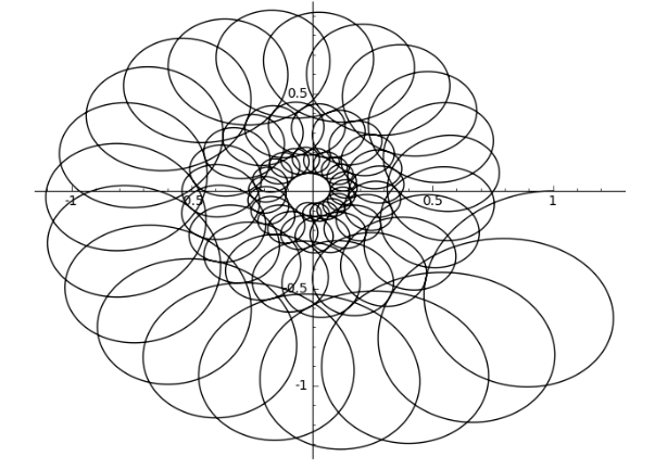
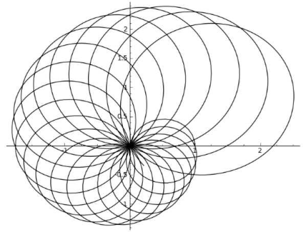
Figure 2. Projections of zero-energy orbits to the $xy$-plane.

Periodic orbits exist and the existence proof forms part of C.S.’s thesis – see Section 5.5 below. We will momentarily report progress with integration of the $H=0$ system, but first we gather other dynamical results.

Proposition 2.

If $H<0$ then any solution is bounded.

Proof.

Suppose $H=-h$ where $h$ is positive. Then $K-U=-h$, so

$$U=K+h\geq h,$$

since $K$ is always non-negative. Then a solution $(x(t),y(t),z(t))$ in configuration space must satisfy

$$0\leq((x^{2}+y^{2})^{2}+\tfrac{1}{16}z)^{1/2}<\frac{\alpha}{h},$$

where $\alpha$ and $h$ are positive constants. ∎

Proposition 3.

The only solutions in the plane $z=0$ are lines through the origin.

Proof.

The equations for $\dot{z}$ and $\dot{\theta}$ satisfy the relation

$$\dot{z}=\tfrac{1}{2}r^{2}\dot{\theta}.$$

For a path lying in the plane $z=0$, this implies either $r=0$ or $\dot{\theta}=0$. In the first case, the path is trivial. In the second, it lies on a line through the origin. Such a curve may be parametrized by

$$\gamma(t)=(c_{1}t^{1/2},c_{2}t^{1/2},0,\tfrac{1}{2}c_{1}t^{-1/2},\tfrac{1}{2}c_{2}t^{-1/2},0).$$

It is easy to verify that the desired equations are satisfied, and that $H=0$. ∎

Proposition 4.

The only solutions constant in configuration space are

$$\gamma(t)=(0,0,k,0,0,-\tfrac{4\alpha}{k^{2}}t).$$

Proof.

This is an easy calculation. Note that such solutions are unbounded in phase space, and satisfy $H<0$. ∎

Next, we explicitly integrate the equations of motion on a codimension 3 submanifold, and recover conics reminiscent of the Euclidean Kepler problem. Consider the smooth submanifold $N=\{z=p_{z}=p_{\theta}=0\}$. This submanifold is invariant under the dynamics, since $\dot{z}=\dot{p}_{z}=\dot{p}_{\theta}=0$ on $N$. The Hamiltonian is

$$H|_{N} =\tfrac{1}{2}p_{r}^{2}-\frac{\alpha}{r^{2}},$$

which has the form of a classical central force problem in the plane. Fix an energy level $H|_{N}=h$. Then since $p_{r}=\dot{r}$, we can explicitly solve for $r(t)$ as follows.

Proposition 5.

On $N$, $r(t)$ traces out a hyperbola if $h>0$, an ellipse if $h<0$, and a parabola if $h=0$.

Proof.

The Hamiltonian may be rewritten as the simple ODE

$$\tfrac{1}{2}\Big{(}\frac{dr}{dt}\Big{)}^{2}=\frac{\alpha}{r^{2}}+h.$$

Assume temporarily that $h\neq 0$. Integrating, we find

$$t =\int dt=\tfrac{1}{\sqrt{2}}\int\frac{r}{\sqrt{\alpha+r^{2}h}}dr=\tfrac{1}{h\sqrt{2}}\sqrt{\alpha+r^{2}h},$$

which may be rewritten $r^{2}-2ht^{2}=-\tfrac{\alpha}{h}.$ Since $\alpha>0$, this curve in the $t,r$-plane is an ellipse for $h<0$ and a hyperbola for $h>0$.

If $h=0$, we find that

$$t=\tfrac{1}{\sqrt{2\alpha}}\int rdr=\tfrac{1}{2\sqrt{2\alpha}}r^{2},$$

and thus $r^{2}=\sqrt{8\alpha}\ t.$ ∎

We conclude this section with the following conjecture:

Conjecture.

There is an open set of initial conditions whose orbits are asymptotic to helices.

This behavior is suggested by numerical experiment and by the fact that $U$ and its derivatives tend to zero as orbits tend towards $\infty$.

5.4. Integration of the case $H=0$

We now focus on the $H=0$ case and reduce the integrability of the equations of motion to the parametrization of a family of degree 6 algebraic plane curves.

Let $\tilde{H}=\frac{K}{U}$. Then integral curves for $\tilde{H}$ are the same as geodesics for the metric $Uds^{2}_{\mathbb{H}}$. When $H=0$, this is the same as the metric $(H+U)ds^{2}_{\mathbb{H}}$, whose geodesics correspond to integral curves for $H$, according to the Jacobi-Maupertuis principle. Thus, the flow of $H$ is the same as the flow of $\tilde{H}$ up to reparametrization on the hypersurface $\{H=0\}=\{\tilde{H}=1\}.$

A short calculation shows that both $J$ and $p_{\theta}$ Poisson commute with $\tilde{H}$. (Recall $\{H,J\}=2H$.) This demonstrates the scale invariance of $\tilde{H}$; $\delta_{\lambda}\colon\tilde{H}\mapsto\tilde{H}.$ More importantly, we have three independent quantities conserved by the flow of $\tilde{H}$. Thus, we have an integrable system on $\{H=0\}=\{\tilde{H}=1\}.$

Change our third coordinate $z\mapsto v=z/r^{2}$. We have conjugate momenta $\tilde{p}_{r},p_{\theta},p_{v}$. In these coordinates, we have $J=r\tilde{p}_{r}$ (as in the Euclidean case) and $\tilde{H}=\tilde{H}(p_{\theta},J,v,p_{v}).$ On the submanifold $\{H=0\}$, we have $\tilde{H}=1$. Also, the initial conditions determine the constants $J$ and $p_{\theta}$. Thus, given initial conditions, $\tilde{H}$ is a function of $v$ and $p_{v}$ only. We arrive at the following result.

Proposition 6.

When $\tilde{H}=1$, any solution must project to an algebraic curve in the $v,p_{v}$-plane.

These curves are naturally degree 10 but can be reduced to degree 6 by changing variables. Examples are shown in Figure  3. If we can parametrize these curves, we should be able to bootstrap up to find explicit solutions.

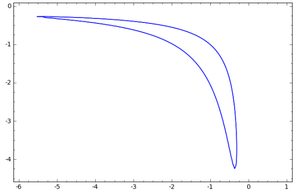
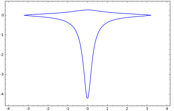
Figure 3. Curves in the $v,p_{v}$-plane corresponding to $J=3,\ p_{\theta}=1$ (left) and $J=0,\ p_{\theta}=1$ (right).

5.5. Periodic Orbits

Despite the fact that the $H=0$ case is integrable, we have not been able to explicitly solve the equations. However, we know that periodic orbits exist.

Take $L=K+U$ as our Lagrangian and impose the horizontal constraint $\dot{z}=\tfrac{1}{2}x\dot{y}-\tfrac{1}{2}y\dot{x}$. Then any trajectory $\gamma$ must lie on the zero set of the function

$$G=\tfrac{1}{2}x\dot{y}-\tfrac{1}{2}y\dot{x}-\dot{z}.$$

The calculus of variations tells us that if $\gamma\colon[0,T]\to\mathbb{H}$ is a minima of the action functional $\int_{0}^{T}Ldt$ which also satisfies our constraint, then there exists a scalar $\lambda=\lambda(t)$ such that $\gamma$ is a minima of the modified action functional

$$A(\gamma)=\int_{0}^{T}L_{\lambda}(t,\gamma,\dot{\gamma})dt,$$

where we have written $L_{\lambda}(t,\gamma,\dot{\gamma})=L(t,\gamma,\dot{\gamma})-\lambda(t)G(t,\gamma,\dot{\gamma})$. Setting the first variation of $A$ equal to zero and integrating by parts yields the Euler-Lagrange equations:

$$\ddot{x} =-\lambda\dot{y}-\tfrac{1}{2}\dot{\lambda}y-2\alpha x(x^{2}+y^{2})\rho^{-6}$$

$$\ddot{y} =\lambda\dot{x}+\tfrac{1}{2}\dot{\lambda}x-2\alpha y(x^{2}+y^{2})\rho^{-6}$$

$$\dot{\lambda} =-\tfrac{\alpha}{16}z\rho^{-6}.$$

When $\lambda=p_{z}$ we find that these agree with Hamilton’s equations.

We are confident that the direct method in the calculus of variations applied to $A(\gamma)$ will yield a proof of the existence of periodic orbits. One works in the Hilbert space $H^{1}(S^{1},\mathbb{H})$ and requires that admissible curves are horizontal and satisfy the symmetry conditions

$$\gamma(t+T/3)=R_{2\pi/3}\gamma(t)$$ (S1)

and

$$z(t+T/2)=-z(t),$$ (S2)

where

$$R_{2\pi/3}=\begin{bmatrix}-\frac{1}{2}&-\frac{\sqrt{3}}{2}&0\\ \frac{\sqrt{3}}{2}&-\frac{1}{2}&0\\ 0&0&1\end{bmatrix}.$$

Any admissible curve is therefore necessarily periodic, with additional symmetry. A suggestive approximation of such a curve is shown in Figure 4.

The idea is to choose a minimizing sequence $\gamma_{n}$ of curves in this space, and show that they converge within the space to some $\gamma_{*}$. Applying elementary analysis and the principle of symmetric criticality shows that $\gamma_{*}$ must minimize the action, thereby satisfying the Euler-Lagrange equations. A central difficulty lies in proving that $\gamma_{*}$ does not pass through the singularity at the origin. A full existence proof is expected to appear in the thesis of C.S.

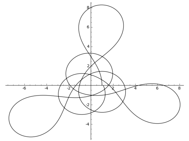
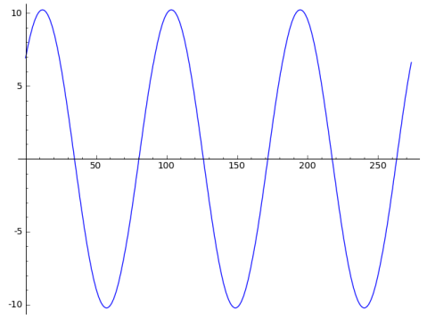
Figure 4. Projection of an orbit to the $xy$-plane (left) and $z$-coordinate over time (right)

5.6. A failure of reduction.

Newton reduced his two-body problem to the Kepler problem in Euclidean space. There is no analogous reduction for the two-body problem on the Heisenberg group, nor is there for the two-body problem on the sphere or in hyperbolic space. We discuss the geometric roots of this failure.

We begin by writing down the Heisenberg two-body problem. Let $q_{1},q_{2}\in\mathbb{H}\cong\mathbb{R}^{3}$ denote the positions of two bodies moving in the Heisenberg group $\mathbb{H}$. Let their masses be $m_{1},m_{2}$. Their individual kinetic energies are

$$K_{i}=\frac{1}{2m_{i}}((P^{(i)}_{X})^{2}+(P^{(i)}_{Y})^{2})$$

where $P^{i}_{X},P^{i}_{Y}$ are the horizontal momenta of each body, as in Section 5.2. The Heisenberg two-body problem is defined by the Hamiltonian

$$H=K_{1}+K_{2}-\kappa m_{1}m_{2}U(q_{1}^{-1}q_{2}),$$

where $\kappa$ is the Gravitational constant and $U$ is Folland’s fundamental solution. $H$ is a Hamiltonian on the cotangent bundle of $\mathbb{H}\times\mathbb{H}$, and is invariant under the (cotangent lift of the left) translation $(q_{1},q_{1})\mapsto(gq_{1},gq_{2})$, $g\in\mathbb{H}$.

We know of two derivations of Kepler’s problem (on Euclidean space) from Newton’s two-body problem. We will call these the ‘algebraic’ and the ‘group-theoretic’ derivations. The ‘algebraic derivation’ begins with the equation $F=ma$ for each body. Divide the equation for each body by its mass to get equation for the acceleration $\ddot{q}_{i}$ of each body’s position vector $q_{i}$. Subtract one equation from the other to obtain the ODE of Kepler’s problem, $\ddot{q}=-\alpha q/|q|^{3},$ for the difference vector $q=q_{1}-q_{2}$. The ‘group theoretic derivation’ depends on the conservation of the total linear momentum, the invariance of Newton’s mechanics with respect to Galilean boosts, and the abelian nature of the translation group. If $P$ is the total linear momentum and $M$ the total mass, we boost by the velocity $-P/M$ to get to a new representation of the same dynamics in which the total linear momentum is zero. Then we reduce by translation at the value $0$ by placing the center of mass at the origin. Finally, we compute that each mass separately satisfies Kepler’s equation with the origin – the center of mass – now playing the role of “sun”.

The algebraic derivation fails on the Heisenberg group because the ‘difference vector’ $g_{1}(t)^{-1}g_{2}(t)$ of two Heisenberg geodesics is not a Heisenberg geodesic. Why is this lack of being a geodesic a problem? Set the Heisenberg Gravitational constant $\kappa=0$ so the two-body problem reduces to two uncoupled Heisenberg geodesic problems. Play the algebraic game. Our ‘difference vector’ does not satisfy the Heisenberg geodesic equations or any other pretty Hamiltonian equation. But in the Newtonian-Euclidean case, the difference vector travels like a free particle, i.e., moves in a straight line – as it should with $\alpha=0$ in Kepler’s problem. Things will just get worse for $\kappa\neq 0$.

The failure of the group theoretic derivation goes a bit deeper and is perhaps more enlightening. What is a ‘Galilean boost’ for an arbitrary Lie group? We choose some ‘translation velocity’ $\xi$ and multiply elements $x_{0}$ by $exp(t\xi)$. Euclidean space enjoys the wonderful property that $exp(t\xi)x_{0}=x_{0}+t\xi$ describes free motion; it is a geodesic. This assertion is decidedly false for the Heisenberg group: the orbits of (left or right) translates of one parameter subgroups are not Heisenberg geodesics. As a result, applying a boost to a solution $(q_{1}(t),q_{2}(t))$ to the Heisenberg two-body problem will not yield a solution. There is a conserved total ‘linear momentum’: the momentum map for the (left) translation action. But we cannot use it to ‘Galilean boost’ the ‘center of mass velocity’ down to zero. Even if this total linear momentum were initially zero, we still seem to be stuck. The non-Abelian nature of the group appears to block us from writing the reduced Hamiltonian at zero as a Kepler Hamiltonian on the ‘diagonal group’ of elements $q=q_{1}^{-1}q_{2}$.

In spherical and hyperbolic geometry, reduction of the two-body problem to the Kepler problem fails for similar reasons. See [7]. In the spherical case, Shchepetilov [16] used the Morales-Ramis theory to prove that the two-body problem in these two geometries is not meromorphically integrable.

Question. Is the two-body problem on the Heisenberg group non-integrable?

6. Kepler’s Problem on a Lattice.

Lattices admit one-sided dilations: we can scale a lattice $\mathbb{L}$ by a positive integer $c$ and land back in the lattice, stretching all distances by $c$. They admit Laplacians. So we might be able to begin to investigate Kepler’s 3rd law on $\mathbb{L}$.

What are Newton’s equations on $\mathbb{L}$? Since we must hop from lattice site to lattice site, we must choose our time variable $t$ to be discrete:

$$t=\ldots,-1,0,1,2,\ldots.$$

A ‘solution’ to Newton’s equations will then be a ‘discrete curve’

$$\gamma:\mathbb{Z}\to{\mathbb{L},}\qquad\mathbb{L}\text{ our lattice,}$$

satisfying a difference equation which mimics Newton’s equations. In 1st order Hamiltonian form these equations should resemble

$$\frac{d\gamma}{d[t]}=p$$

$$\frac{dp}{d[t]}=-\nabla V(\gamma(t)),$$

where the differential is the discrete difference operator

$$\frac{d\gamma}{d[t]}=\gamma(t+1)-\gamma(t),$$

and where $V:\mathbb{L}\to\mathbb{R}$ is our potential. The standard interpretation of $\nabla V$ is in terms of its differential

$$dV(\ell):\mathbb{E}_{\ell}\to\mathbb{R},\quad\ell\in\mathbb{L},$$

where $\mathbb{E}=\mathbb{E}_{\ell}$ is the set of edges (chosen lattice generatos) leaving the lattice site $\ell,$ and where

$$dV(\ell)(e)=V(\ell^{\prime})-V(\ell),\quad e=[\ell,\ell^{\prime}]\text{ an edge}.$$

Then we can rewrite our Newton difference equations as

$$\gamma(t+1)=\gamma(t)+p(t)$$ (4)

$$p(t+1)=p(t)-dV(\gamma(t)).$$ (5)

What is the momentum, $p(t)$? We add to it $dV(\gamma(t))$, so it must lie in the same space as $dV,$ which is

$$\mathbb{E}^{*}=\mathbb{E}_{\ell}^{*}=\text{ real valued functions on }\mathbb{E}_{\ell}.$$

This ‘cotangent space at $\ell$’ is a vector space isomorphic to $\mathbb{R}^{d},$ where $d$ is the degree of a vertex: the number of edges leaving $\ell$. Good. Now, how do we add $p(t)\in\mathbb{E}^{*}$ to a lattice site $\ell=\gamma(t)\in\mathbb{L}$ in order to get a new lattice site $\gamma(t+1)$ as in the 1st Newton equation? We seem to be missing the ‘mass matrix’ or ‘cometric’ of mechanics.

Definition 2.

A lattice cometric is a ‘non-trivial’ map

$$\mathbb{M}:\mathbb{E}^{*}\to\mathbb{L}.$$

With this tentative definition we can now try to write down ‘Newton’s equations’

$$\gamma(t+1)=\gamma(t)+\mathbb{M}(p(t))$$ (6)

$$p(t+1)=p(t)-dV(\gamma(t)),$$ (7)

which define a discrete dynamics on the phase space $\mathbb{L}\times\mathbb{E}^{*}.$ The resulting dynamics have some vague relation to the corresponding formal Hamiltonian

$$H(\ell,p)=\frac{1}{2}p\mathbb{M}p+V(\ell),$$

but we aren’t sure how to interpret the term $p\mathbb{M}p$.

7. Kepler’s problem on $\mathbb{Z}$.

The Laplacian $\Delta$ on $\mathbb{Z}$ is given by $\Delta f(n)=f(n+1)-2f(n)+f(n-1)$.

Exercise. Show that $U(n)=-\frac{1}{2}|n|$ is a fundamental solution for the Laplacian on $\mathbb{Z}$ with source at $S=0$.

Take the Kepler constant $\alpha=2$ so that the ‘Newtonian potential’ $V=-\alpha U$ is $V=|n|.$ The Hamiltonian is

$$H(n,p)=\frac{1}{2}p^{2}+|n|.$$

Since $\frac{d}{d[n]}|n|=sgn(n)$ is the sign of $n$, $1$ if $n>0$ and $-1$ if $n\leq 0$, we find that with this choice of $\alpha$ the discrete gradient is integer valued. We get a good discrete dynamical system. Newton’s equations (in 1st order form) become

$$n(j+1)=n(j)+p(j)$$

$$p(j+1)=p(j)-sgn(n).$$

A solution is depicted in Figure 5.

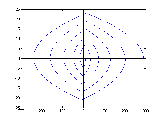
Figure 5. A Kepler orbit in integer phase space

At each iteration, the ‘lattice momentum’ $p$ decreases by one as long as $n>0$ and increases by $1$ as long as $n<0$. (We have to make a choice at $n=0$; above we chose $sgn(0)=-1.$) Note that as long as the initial condition $p(0)$ is an integer, it remains an integer, and we stay on the lattice!

Because of this happy coincidence with $p$’s evolution, we did not need to worry about where $p$ lived. It is a real number that happens to evolve to stay integral. Our momentum space is not $\mathbb{E}^{*}\cong\mathbb{R}^{2}$. (There are two directions, right and left, on the lattice, hence the dimension 2.) We also did not need to choose a ‘lattice cometric’ $\mathbb{M}$. If any choice was made, it seems to have been ‘$1$’ as written in the Hamiltonian. The happy coincidence does not happen when we go up to the rank 2 lattice.

7.1. Kepler on the rank 2 lattice.

The rank 2 lattice is $\mathbb{Z}^{2}$ with elements written $\ell=(n,m)$. As a metric space, we use the distance

$$d((n,m),(n^{\prime},m^{\prime})=|n-n^{\prime}|+|m-m^{\prime}|.$$

The Laplacian is

$$\Delta f(\ell)=\sum_{\ell^{\prime}:\ d(\ell,\ell^{\prime})=1}(f(\ell^{\prime})-f(\ell)).$$

Let $U$ denote the fundamental solution, this being the ‘most bounded’ solution to $\Delta U=\delta_{0}$, where $\delta_{0}$ is the lattice delta function corresponding to placing the sun at the origin. (There is a lattice Liouville theorem, so $U$ can be made unique up to an additive constant.) There is no closed form expression for $U.$ However, any particular value of $U$ can be computed recursively. Indeed, the fundamental solution is a well studied object with applications to the theory of electrical circuits ([4]), solid state physics, and quantum mechanics. Some values of the lattice Green’s function are reproduced in Figure 6 from [10]. (We thank the brothers Hollos for permission to reproduce their table.)

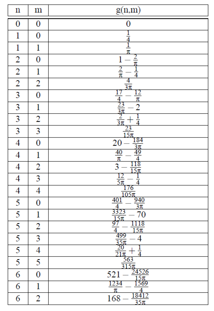
Figure 6. Values of the Green’s function $g$ on $\mathbb{Z}^{2}$, taken from [10]

We write the formal Hamiltonian

$$H(\ell,p)=\frac{1}{2}p\mathbb{M}p-\alpha U(\ell)$$

and derive Hamilton’s equations

$$\ell(t+1)=\ell(t)+\mathbb{M}p(t)$$

$$p(t+1)=p(t)+\alpha dU(\ell(t))$$

where

$$\mathbb{M}:\mathbb{R}^{4}=\mathbb{E}^{*}\to\mathbb{Z}^{2}.$$

The vector $p$ is a 4-vector with components $(p_{up},p_{down},p_{right},p_{left})$ corresponding to the 4 edges, which are the 4 directions of motion, through each vertex. We have, for example $dU(\ell)_{up}=U(\ell+e_{2})-U(\ell)$ where $e_{2}=(0,1)$ represents motion in the ‘up’ direction. The second Hamilton equation makes sense.

When we try to parse the first Hamilton equation we get stuck. What do we take for $\mathbb{M}:\mathbb{R}^{4}\to\mathbb{Z}^{2}$? We require $\mathbb{M}$ to be non-constant. Certainly $\mathbb{M}$ will not be continuous! Ideally $\mathbb{M}$ is ‘linear’:

$$\mathbb{M}(kp)=k\mathbb{M}(p),\quad k\in\mathbb{Z},$$

but this is probably not possible in any reasonable sense. One possibility for $\mathbb{M}$ is to argue that there is a ‘canonical’ projection $\Pi:\mathbb{R}^{4}\to\mathbb{R}^{2}$, for example, $\Pi(p_{up},p_{down},p_{right},p_{left})=\frac{1}{2}(p_{up}+p_{down},p_{right}+p_{left})$, and a canonical embedding of our lattice as $\mathbb{Z}^{2}\subset\mathbb{R}^{2}$. Then choose $\mathbb{M}(p)$ to be the lattice point closest to $\Pi(p)$. This leaves us to worry about what to do if $\Pi(p)$ is midway between lattice points. Flip a coin?

We are stuck and look forward to some of our readers unsticking us.

7.1.1. Euler-Lagrange formulation.

We can make a bit more sense of the Euler Lagrange version of lattice dynamics. Fix a positive integer $T$, the ‘time of flight,’ and initial and final vertices, $v_{0},v_{1}\in\mathbb{Z}^{2}$. There will be two formulations. In both, we consider discrete paths $\gamma:\{0,1,\ldots,T\}\to\mathbb{Z}^{2}$ which join $v_{0}$ to $v_{1}$ in time $T$, and we minimize an ‘action functional’ $A$ among all such discrete paths.

Version 1: Minimize the action

$$A(\gamma)=\sum_{t=0}^{T}\{\frac{1}{2}(|\frac{d}{d[t]}\gamma(t)|_{1})^{2}+\alpha U(\gamma(t))\}$$

among all discrete paths $\gamma$ joining $v_{0}$ to $v_{1}$ in discrete time $T$.

Here $|\frac{d}{d[t]}\gamma(t)|_{1}=d(\gamma(t+1),\gamma(t)),$ so half of its square represents kinetic energy.

Version 2: Call a discrete path ‘continuous’ if either $d(\gamma(t+1),\gamma(t))=1$ or $\gamma(t+1)=\gamma(t)$. Minimize the same action as Version 1, but now over all continuous paths. (In this case the kinetic term $\frac{1}{2}(|\frac{d}{d[t]}\gamma(t)|_{1})^{2}$ is either $1/2$ or $0$ at each time step.)

We are guaranteed a solution to Version 2 exists since there are only a finite number of ‘continuous’ paths joining $v_{0}$ to $v_{1}$. We suspect that if we move too fast the kinetic energy becomes too large, so that Version 1 is ‘coercive’ and one can argue that again there are only a finite number of paths that matter.

It seems doubtful that any decent Euler-Lagrange type difference equation ‘dynamics’ will result from either principle. Indeed, take the case $\alpha=0$ of a ‘free particle’ on the latttice, and take $v_{0}=(0,0),\ v_{1}=(n,m)$, $n>m\geq 0$. There are $(n+1)m$ shortest paths from $v_{0}$ to $v_{1}$. Just draw box-paths, always moving either right or up. Their lengths are all $n+m=d(v_{0},v_{1})$. If $T<d(v_{0},v_{1})$ then there are no paths connecting the two points. If $T=d(v_{0},v_{1})$ then their actions are all $\frac{1}{2}T$. If $T>d(v_{0},v_{1})$ the action remains the same; we just stay still for the requisite times $T-d(v_{0},v_{1})$. This means either (i) all points $v_{1}=(n,m)$ with $nm\neq 0$ are conjugate to $v_{0}$, or (ii) that there is no good ‘free’ dynamical equation, so likely no good Euler-Lagrange equations in general.

8. Quantum Mechanics to Classical Mechanics on Cayley Graphs?

By a graph here we mean the usual combinatorial collection of vertices and edges. We write $\Gamma$ for the set of vertices and view $\Gamma$ as ‘configuration space.’ The graph Laplacian is the operator $\Delta:\ell_{2}(\Gamma)\to\ell_{2}(\Gamma)$ defined by

$$\Delta f(v)=\sum_{v^{\prime}:[v,v^{\prime}]\text{ an edge}}(f(v^{\prime})-f(v)).$$

If $\Gamma$ is finite there will be no fundamental solution; that is, there is no solution to $\Delta U_{S}=\delta_{S}$ where where $\delta_{S}$ is the discrete $\delta$ function centered at the sun: $\delta_{S}(S)=1,\delta_{S}(v)=0,v\neq S$. If $\Gamma$ is finite, a necessary condition for the solvability of $\Delta V=f$ is $\Sigma f(v)=0$, which will fail for $f=\delta_{S}$.

Regardless of whether or not $\Gamma$ has a Green’s function, it has plenty of potentials, meaning functions $V\in\ell_{2}(\Gamma)$. Consequently for each choice of Planck’s constant $\hbar$ we have a Schrodinger operator:

$$\hbar^{2}\Delta+V:\ell_{2}(\Gamma)\to\ell_{2}(\Gamma).$$

There is a large active field of graph Laplacians and quantum mechanics on graphs. There is undoubtedly a theory of quantum mechanics on $\Gamma$.

Challenge. Don’t you think this quantum mechanics ought to have a classical limit? If ‘yes’ then please answer: what are the correct Newton’s equations for an arbitrary potential, on an arbitrary graph?

8.0.1. Cayley graph of a group

Let $\Gamma$ be a finitely generated group and $e_{1},\ldots,e_{d}\in\Gamma$ be a fixed set of generators for $\Gamma$ (so every element of $\Gamma$ is a product of the $e_{i}$’s or their inverses). Form the graph whose vertices are the elements $x\in\Gamma$ and for which two vertices $x,y\in\Gamma$ are joined by an edge if and only if either $y=xe_{i}$ or $x=ye_{i}$ for some generator $e_{i}$. Count each edge as having length $1$. Define the distance between points $x$ and $y$ in $\Gamma$ to be the minimum of the lengths of the paths joining $x$ to $y$. This distance is always an integer, since the length of a path is just the number of edges it contains.

In this representation, the ‘Lie algebra’ of the Cayley graph will be the tangent space at the identity: the disjoint union of $d$ copies of $\mathbb{Z}$. Alternatively, it is the subset of $\mathbb{Z}^{d}$ consisting of vectors for which all but one component is zero.

Example: Lattices. Take $\Gamma=\mathbb{Z}^{2}$ to be the lattice of integers in the plane, with standard generators $e_{1}=(1,0),e_{2}=(0,1)$. Then the Cayley graph of $\mathbb{Z}^{2}$ realized as above has the vertices of a standard infinite sheet of graph paper in $\mathbb{R}^{2}$. Its Lie algebra consists of integer points on the $x$-axis unioned with the collection of integer points on the $y$-axis.

8.0.2. Kepler symmetries of Cayley graphs.

Every Cayley graph satisfies Keplerian symmetry property (1) of being homogeneous since $\Gamma$ acts on itself on the right by isometries. View the generators as the ‘directions.’ Then if the automorphism group of the group $\Gamma$ acts transitively on its generating set $e_{1},\ldots,e_{d},$ the metric is isotropic; it satisfies Keplerian symmetry property (2). Finally we can send $e_{i}$ to $e_{i}^{k}$. In some instances this defines a group homomorphism of $\Gamma$ into itself. Then the Cayley graph admits one-sided dilations and so satisfies (3). The examples we know of groups whose Cayley graphs satisfy (1), (2) and (3) are the lattices $\mathbb{Z}^{d}$, the lattices in nilpotent groups, and the free group on $d$ generators. In the continuous case, we know how to derive a Kepler’s third law from the Keplerian symmetry (3). Is there an analogous construction in the discrete case?

8.0.3. Full Disclosure – R.M.

I have little interest in any kind of graph for its own sake. I am not a combinatorist, nor a discrete group theorist!

In contrast to the dozens of books that Jerry wrote in his life, I have mustered the courage and stamina to write a single book in this life. (Jerry continues to amaze.) In that book I devoted a chapter to trying to understand one of the big ideas of Gromov in his paper ‘On Groups of Polynomial Growth …’ ([8]) in which he used subRiemannian ideas to solve a problem in discrete group theory. Consider a discrete finitely generated group $\Gamma$. Select some generators and form the group’s Cayley graph. We say the group is ‘of polynomial growth’ if the number of vertices of the Cayley graph lying inside a ball of radius $R$ is bounded by a polynomial in $R$ as $R\to\infty$. (If $\Gamma$ is of polynomial growth with respect to one set of generators, it is of polynomial growth with respect to any other set of generators.) The lattices, and the integer lattice in the Heisenberg group are examples of groups of polynomial growth. More generally, the lattices in any Carnot group are of polynomial growth. The free group on 2 generators in not of polynomial growth: its balls have exponential growth, roughly $3^{R}$. There is a notion of a group being ‘virtually nilpotent,’ and it was known that virtually nilpotent implies polynomial growth. Gromov proved the converse: polynomial growth implies virtually nilpotent.

Gromov’s paper is mind-blowing – the most astounding application of subRiemannian geometry that I know of made by a human. (Cats and micro-organisms have made their own astounding applications.) Gromov scales the edges of the Cayley graph by $\epsilon$, then takes the limit as $\epsilon\to 0$. He proves, in essence, that the result converges to a Carnot group – a metric of subRiemannian type on a nilpotent Lie group – and from this the theorem easily follows. (I am stretching the truth here, but that is the spirit of Gromov’s paper. There are many technicalities.) What I find so compelling about Gromov’s paper is the going back and forth between the wonderful world of smooth metric spaces – Lie groups even – which I know and love, and the chopped up world of discrete objects that I find so frightening at times. Can we similarly go back and forth in dynamics? That is what I would like to see in some ‘Kepler problem on a lattice.’

References

- [1] R. Abraham and J.E. Marsden, Foundations of Mechanics, Benjamin-Cummings, (1978).
- [2] V.I. Arnold, V.V. Kozlov, and A.I. Neishtadt, Mathematical Aspects of Classical and Celestial Mechanics, 3rd Ed., Springer-Verlag, (2010).
- [3] A. Albouy, Projective dynamics and classical gravitation, arXiv:math-ph/0501026v2, (2005).
- [4] J. Cserti, Application of the lattice Green’s function for calculating the resistance of infinite networks of resistors, Am.J.Phys.68:896-906, arXiv:cond-mat/9909120v4, (2000).
- [5] G. Folland, A fundamental solution for a subelliptic operator, Bulletin of the AMS, 79, (1973).
- [6] F. Diacu, E. Perez-Chavela, and M. Santoprete, The n-body problem in spaces of constant curvature, arXiv:0807.1747v6 [math.DS], (2008).
- [7] F. Diacu, The non-existence of centre-of-mass and linear-momentum integrals in the curved N-body problem, arXiv:1202.4739v1 [math.DS], (2012).
- [8] M. Gromov, Groups of polynomial growth and expanding maps, Publ. Math. IHES, 53 (1981), 53-73.
- [9] M. Gromov, Metric Structures for Riemannian and Non-Riemannian Spaces, Birkhauser, 3rd printing, (2007).
- [10] S. Hollos and R. Hollos, The lattice Green function for the Poisson equation on an infinite square lattice, arXiv:cond-mat/0509002v1 [cond-mat.other], (2005).
- [11] N. I. Lobachevsky, The new foundations of geometry with full theory of parallels [in Russian], 1835-1838, In Collected Works, V. 2, GITTL, Moscow, (1949), p. 159.
- [12] J. E. Marsden and M. West, Discrete mechanics and variational integrators, Acta Numerica, 10 (2001), 357-514.
- [13] R. Moeckel and R. Montgomery, Symmetric regularization, reduction and blow-up of the planar three-body problem, arXiv:1202.0972v1 [math.CA], (2012).
- [14] R. Montgomery, A Tour of Subriemannian Geometries, AMS, (2002).
- [15] P.J. Serret, Théorie nouvelle géométrique et mécanique des lignes a double courbure, Librave de Mallet-Bachelier, Paris, (1860).
- [16] A. Shchepetilov, Nonintegrability of the two-body problem in constant curvature spaces, arXiv:math/0601382v3 [math.DS], (2006).