Detecting modified vacuum fluctuations due to presence of a boundary by means of the geometric phase

Abstract

We study the geometric phase acquired by an inertial atom whose trajectories are parallel to a reflecting boundary due its coupling to vacuum fluctuations of electromagnetic fields, by treating the atom as an open quantum system in a bath of the fluctuating vacuum fields, and show that the phase is position dependent as a result of the presence of the boundary which modifies the field quantum fluctuations. Our result therefore suggests a possible way of detecting vacuum fluctuations in experiments involving geometric phase.

Quantum theory has profoundly changed our conception of vacuum as a synonym of nothingness. As an inevitable consequence necessitated by the uncertainty principle, vacuum fluctuates and thus may have rich structures. An intriguing issue is what are the physical consequences of vacuum fluctuations that exist all the time and whether these fluctuations can be directly detected. In this regard, let us note that the effects of vacuum fluctuations in free space may not be always observable, let alone a direct observation, since some physical quantities, energy for instance, are not well-defined in vacuum and one has to invoke certain renormalization schemes to make them finite. However, changes in the vacuum fluctuations, e.g., those caused by the presence of boundaries, usually exhibit normal behaviors and can produce observable effects. The Lamb shift lamb and the Casimir casimir1 (and the Casimir-Polder casimir2 ; casimir3 ) effects are the two most well-known examples, which have been precisely measured. Other examples of novel effects that arise as a result of the vacuum fluctuations include but are by no means limited to the light-cone fluctuations when gravity is quantized lightcone , the Brownian motion of test particles in an electromagnetic vacuum brown , and modifications of radiative properties of atoms in cavities such as the natural lifetimes and energy level shifts which have been demonstrated in experiments cavity . In this paper, we show that the vacuum fluctuations may also be directly detected though the measurement of geometric phase. As a related issue of vacuum fluctuation detection, it is worth noting that the quantum vacuum fluctuation in the position of a mechanical system has recently been clearly detected using a nanomechanical resonator AHS .

The geometric phase is an important concept in quantum theory. In 1984, Berry studied the dynamics of a closed quantum system whose Hamiltonian varies adiabatically in a cyclic way, and found that there is, besides the familiar dynamical phase, an additional phase due to the geometry of the path enclosed during the unitary evolution of the system in the parameter space berry . Ever since the inception, the geometric phase has aroused broad interest and has been extensively studied, both theoretically and experimentally GPbook . Recent concerns about the geometric phase mainly focus on its potential of performing fault-tolerant quantum computation fault-tolerant . Because of the inevitable interactions between the qubits and the environment, a pure state will generically be driven to a mixed state. To deal with the effect of the environment, many attempts have been made which generalize the geometric phase of a closed system undergoing a unitary evolution to an open quantum system which undergoes a nonunitary one Uhlmann ; Sjoqvist ; Singh ; Tong ; Wang . Remarkably, experiments have demonstrated both the geometric phase of a mixed state undergoing a cyclic unitary evolution  Du ; Marie and that of an open system undergoing nonunitary one critical .

In fact, the impact of environment on the geometric phase is a crucial issue in any practical implementations of quantum computing. The effects of different kinds of decoherence sources on the geometric phase have been analyzed Carollo ; Rezakhani ; Lombardo ; chen ; Marzlin . It is remarkable that when the temperature is absolute zero, there is still a correction to the geometric phase caused by the environment, i.e., a reservoir of vacuum fluctuations Lombardo ; chen ; Marzlin . However, this kind of inevitable vacuum fluctuation induced geometric phase is in general unobservable, since any phase variation is observed usually via some kind of interferometry between the involved state and certain selected reference states which are both inseparably and equally coupled to vacuum. Nevertheless, if, somehow, vacuum fluctuations are modified, then the geometric phase of the nonunitary evolution of an open system caused by its coupling to vacuum may become potentially observable. Here, we show that the modification of vacuum fluctuations induced by the presence of boundaries provides such a possibility to unveiling quantum vacuum fluctuations via geometric phase. At this point, it is worth noting that geometric phase has recently been proposed as a possible way to detect the Unruh effect in Ref. Martin and later in Ref. HuYu .

The system we study contains an inertial two-level atom in interaction with a bath of fluctuating quantum electromagnetic fields in vacuum at a fixed distance to a reflecting boundary. The Hamiltonian of the whole system takes the form $H=H_{s}+H_{\phi}+H^{\prime}.$ Here $H_{s}$ is the Hamiltonian of the atom, which, for simplicity, is taken to be $H_{s}={1\over 2}\,\hbar\omega_{0}\sigma_{3},$ where $\sigma_{3}$ is the Pauli matrix, and $\omega_{0}$ is the energy-level spacing of the atom. $H_{\phi}$ is the Hamiltonian of the electromagnetic field, of which the explicit form is not relevant here. In the multipolar coupling scheme CPP95 , the interaction Hamiltonian $H^{\prime}$ takes the form $H^{\prime}(\tau)=-e\,\textbf{r}\cdot\textbf{E}(x(\tau))=-e\sum_{mn}\textbf{r}_{mn}\cdot\textbf{E}(x(\tau))\sigma_{mn},$ where e is the electron electric charge, $e\,\bf r$ the atomic electric dipole moment, and ${\bf E}(x)$ the electric-field strength. Here, the dipole moment must be kept fixed with respect to the proper frame of reference of the atom; otherwise, the rotation of the dipole moment will bring in extra time dependence in addition to the intrinsic time evolution Takagi . Since neither r nor $\textbf{E}(x)$ is a world vector, the interaction Hamiltonian $H^{\prime}$ is ambiguous when we deal with the situation of moving atoms. However, we can write the interaction Hamiltonian $H^{\prime}$ in a coordinate invariant form as $H^{\prime}=-e\,r^{\mu}F_{\mu\nu}(x)\,u^{\nu}$, where $F_{\mu\nu}$ is the field strength, $r^{\mu}$ is a four-vector such that its temporal component in the frame of the atom vanishes and its spatial components in the same frame are given by r, and $u^{\nu}$ is the four velocity of the atom. Since we choose to work in the frame of the atom, $u^{\nu}=(c,0,0,0)$, and this coordinate invariant interaction Hamiltonian reduces to the form given above Takagi ; Borde . The dynamical evolution of the two-level-atom subsystem will be studied in the paradigm of open quantum systems. Here, let us note that the theory of open quantum systems has been fruitfully applied to understand, from a perspective different from the traditional, the Unruh, Hawking and Gibbons-Hawking effects, in Refs. Benatti1 , yu3 , and yu4 , respectively.

The initial state of the whole system is characterized by the total density matrix $\rho_{tot}=\rho(0)\otimes|0\rangle\langle 0|$, in which $\rho(0)$ is the initial reduced density matrix of the atom, and $|0\rangle$ is the vacuum state of the field. In the frame of the atom, the evolution in the proper time $\tau$ of the total density matrix $\rho_{tot}$ satisfies

$$\frac{\partial\rho_{tot}(\tau)}{\partial\tau}=-{i\over\hbar}[H,\rho_{tot}(\tau)]\;.$$ (1)

We assume that the interaction between the atom and the field is weak. In the limit of weak coupling, the evolution of the reduced density matrix $\rho(\tau)$ can be written in the Kossakowski-Lindblad form Lindblad ; Benatti1 ; Benatti2 ; pr5

$${\partial\rho(\tau)\over\partial\tau}=-{i\over\hbar}\big{[}H_{\rm eff},\,\rho(\tau)\big{]}+{\cal L}[\rho(\tau)]\ ,$$ (2)

where

$${\cal L}[\rho]={1\over 2}\sum_{i,j=1}^{3}a_{ij}\big{[}2\,\sigma_{j}\rho\,\sigma_{i}-\sigma_{i}\sigma_{j}\,\rho-\rho\,\sigma_{i}\sigma_{j}\big{]}\ .$$ (3)

The matrix $a_{ij}$ and the effective Hamiltonian $H_{\rm eff}$ are determined by the Fourier and Hilbert transforms of the correlation functions,

$$G^{+}(x-y)={e^{2}\over\hbar^{2}}\sum_{i,j=1}^{3}\langle-|r_{i}|+\rangle\langle+|r_{j}|-\rangle\,\langle 0|E_{i}(x)E_{j}(y)|0\rangle\;,$$ (4)

which are defined as follows:

$${\cal G}(\lambda)=\int_{-\infty}^{\infty}d\tau\,e^{i{\lambda}\tau}\,G^{+}\big{(}x(\tau)\big{)}\;,$$ (5)

$${\cal K}(\lambda)=\frac{P}{\pi i}\int_{-\infty}^{\infty}d\omega\ \frac{{\cal G}(\omega)}{\omega-\lambda}\;.$$ (6)

Then the coefficients of the Kossakowski matrix $a_{ij}$ can be expressed as

$$a_{ij}=A\delta_{ij}-iB\epsilon_{ijk}\delta_{k3}-A\delta_{i3}\delta_{j3}\;,$$ (7)

in which

$$A=\frac{1}{4}[{\cal G}(\omega_{0})+{\cal G}(-\omega_{0})]\;,\;~{}~{}~{}B=\frac{1}{4}[{\cal G}(\omega_{0})-{\cal G}(-\omega_{0})]\;.$$ (8)

The effective Hamiltonian $H_{\rm eff}$ contains a correction term, the so-called Lamb shift, and one can show that it is given by replacing $\omega_{0}$ in $H_{s}$ with a renormalized energy-level spacing $\Omega$ as follows Benatti1 :

$$H_{\rm eff}=\frac{1}{2}\hbar\Omega\sigma_{3}={\hbar\over 2}\{\omega_{0}+{i\over 2}[{\cal K}(-\omega_{0})-{\cal K}(\omega_{0})]\}\,\sigma_{3}\;.$$ (9)

Assuming the initial state of the atom is $|\psi(0)\rangle=\cos{\theta\over 2}|+\rangle+\sin{\theta\over 2}|-\rangle$, one can show that the time-dependent reduced density matrix of the atom is given by

$$\rho(\tau)=\left(\begin{array}[]{ccc}e^{-4A\tau}\cos^{2}{\theta\over 2}+{B-A\over 2A}(e^{-4A\tau}-1)&{1\over 2}e^{-2A\tau-i\Omega\tau}\sin\theta\\ {1\over 2}e^{-2A\tau+i\Omega\tau}\sin\theta&1-e^{-4A\tau}\cos^{2}{\theta\over 2}-{B-A\over 2A}(e^{-4A\tau}-1)\end{array}\right)\;,$$ (10)

which evolves nonunitarily. The geometric phase for a mixed state under a nonunitary evolution can be defined as Tong

$$\gamma_{g}=\arg\left(\sum\limits_{k=1}^{N}\sqrt{\lambda_{k}(0)\lambda_{k}(T)}\langle\phi_{k}(0)|\phi_{k}(T)\rangle e^{-\int_{0}^{T}\langle\phi_{k}(\tau)|\dot{\phi}_{k}(\tau)\rangle d\tau}\right)\;,$$ (11)

where $\lambda_{k}(\tau)$ and $|\phi_{k}(\tau)\rangle$ are the eigenvalues and eigenvectors of the reduced density matrix $\rho(\tau)$. In order to find the geometric phase, we first calculate the eigenvalues of the density matrix (10) to get $\lambda_{\pm}(\tau)={1\over 2}(1\pm\eta)\;,$ in which $\eta=\sqrt{\rho_{3}^{2}+e^{-4A\tau}\sin^{2}\theta}$ and $\rho_{3}=e^{-4A\tau}\cos\theta+{B\over A}(e^{-4A\tau}-1)$. It is easy to see that $\lambda_{-}(0)=0$. As a result, contribution only comes from the eigenvector corresponding to $\lambda_{+}$ ,

$$|\phi_{+}(\tau)\rangle=\sin{\theta_{\tau}\over 2}|+\rangle+\cos{\theta_{\tau}\over 2}e^{i\Omega\tau}|-\rangle\;,$$ (12)

where

$$\tan{\theta_{\tau}\over 2}=\sqrt{\eta+\rho_{3}\over\eta-\rho_{3}}\;.$$ (13)

The geometric phase can then be calculated directly using Eq. (11),

$$\gamma_{g}=-\Omega\int_{0}^{T}\cos^{2}{\theta_{\tau}\over 2}\,d\tau\;.$$ (14)

Now, we calculate the geometric phase of an atom in the vicinity of a reflecting boundary. To do so, we need the two point functions for the electric fields, which can be found from those of the four-potentials,

$$D^{\mu\nu}(x,x^{\prime})=\langle 0|A^{\mu}(x)A^{\nu}(x^{\prime})|0\rangle=D_{0}^{\mu\nu}(x,x^{\prime})+D_{b}^{\mu\nu}(x,x^{\prime})\;,$$ (15)

in which $D_{0}^{\mu\nu}(x,x^{\prime})$ is the two point function in the Minkowski vacuum without boundaries, and $D_{b}^{\mu\nu}(x,x^{\prime})$ is the correction induced by the presence of the boundary which can be calculated using the method of images. In the Feynman gauge, we have, at a distance $z$ from the boundary,

$$D_{0}^{\mu\nu}(x,x^{\prime})={\hbar\over 4\pi^{2}\varepsilon_{0}c}{\eta^{\mu\nu}\over{[(ct-ct^{\prime}-i\varepsilon)^{2}-(x-x^{\prime})^{2}-(y-y^{\prime})^{2}-(z-z^{\prime})^{2}]}}\;,$$ (16)

$$D_{b}^{\mu\nu}(x,x^{\prime})=-{\hbar\over 4\pi^{2}\varepsilon_{0}c}{{\eta^{\mu\nu}+2n^{\mu}n^{\nu}}\over{[(ct-ct^{\prime}-i\varepsilon)^{2}-(x-x^{\prime})^{2}-(y-y^{\prime})^{2}-(z+z^{\prime})^{2}]}}\;,$$ (17)

where $\eta^{\mu\nu}=diag(1,-1,-1,-1)$, $n^{\mu}=(0,0,0,1)$, and $\varepsilon\rightarrow+0$. The electric field two-point functions can be expressed as a sum of the Minkowski vacuum term and a correction term due to the boundary:

$$\langle E_{i}(x(\tau))E_{j}(x(\tau^{\prime}))\rangle=\langle E_{i}(x(\tau))E_{j}(x(\tau^{\prime}))\rangle_{0}+\langle E_{i}(x(\tau))E_{j}(x(\tau^{\prime}))\rangle_{b}\;,$$ (18)

where

$$\langle 0|E_{i}(x(\tau))E_{j}(x(\tau^{\prime}))|0\rangle_{0} = {\hbar c\over 4\pi^{2}\varepsilon_{0}}(\partial_{0}\partial_{0}^{\prime}\delta_{ij}-\partial_{i}\partial_{j}^{\prime})$$ (19)

$$\times{1\over(x-x^{\prime})^{2}+(y-y^{\prime})^{2}+(z-z^{\prime})^{2}-(ct-ct^{\prime}-i\varepsilon)^{2}}\;,$$

$$\langle 0|E_{i}(x(\tau))E_{j}(x(\tau^{\prime}))|0\rangle_{b} = -{\hbar c\over 4\pi^{2}\varepsilon_{0}}[\,(\delta_{ij}-2n_{i}n_{j})\,\partial_{0}\partial_{0}^{\prime}-\partial_{i}\partial_{j}^{\prime}\,]$$ (20)

$$\times{1\over(x-x^{\prime})^{2}+(y-y^{\prime})^{2}+(z+z^{\prime})^{2}-(ct-ct^{\prime}-i\varepsilon)^{2}}\;.$$

Here $\partial^{\prime}$ denotes the differentiation with respect to $x^{\prime}$.

Let us now consider an atom moving in the $x$-direction with a constant velocity $v$ at a distance $z$ from the plane, so the trajectory is given by

$$t(\tau)=\gamma\tau\;,\ \ \ x(\tau)=x_{0}+v\gamma\tau\;,\ \ \ y(\tau)=y_{0}\;,\ \ \ z(\tau)=z\;,$$ (21)

where $\gamma=(1-v^{2}/c^{2})^{-{1\over 2}}$. Here let us note that the electric-field two-point functions Eqs. (18)-(20), and the trajectory Eq. (21) are described in the laboratory frame. Since the evolution of the atom is studied in the frame of the atom, a Lorentz transformation is required to get the electric field two-point functions in the proper frame of the atom from Eq. (18) to Eq. (20):

$$\langle 0|E_{i}(x(\tau))E_{j}(x(\tau^{\prime}))|0\rangle_{0}={\hbar c\over\pi^{2}\varepsilon_{0}}{\delta_{ij}\over(c\,\Delta\tau-i\varepsilon)^{4}}\;,$$

$$\langle 0|E_{x}(x(\tau))E_{x}(x(\tau^{\prime}))|0\rangle_{b}=\langle 0|E_{y}(x(\tau))E_{y}(x(\tau^{\prime}))|0\rangle_{b}=-{\hbar c\over\pi^{2}\varepsilon_{0}}{c^{2}\Delta\tau^{2}+4z^{2}\over[\;(c\,\Delta\tau-i\varepsilon)^{2}-4z^{2}]^{3}}\;,$$

$$\langle 0|E_{z}(x(\tau))E_{z}(x(\tau^{\prime}))|0\rangle_{b}={\hbar c\over\pi^{2}\varepsilon_{0}}{1\over[\;(c\,\Delta\tau-i\varepsilon)^{2}-4z^{2}]^{2}}\;.$$ (22)

The correlation function and its Fourier transform can be calculated as follows:

$$G^{+}(x)=\sum_{i}{e^{2}\over\hbar^{2}}\,|\langle-|r_{i}|+\rangle|^{2}\langle 0|E_{i}(x)E_{i}(y)|0\rangle\;,$$ (23)

$${\cal G}(\lambda)=\sum_{i}{e^{2}|\langle-|r_{i}|+\rangle|^{2}\lambda^{3}\over 3\pi\varepsilon_{0}\hbar c^{3}}(1-f_{i}(\lambda,z))\theta(\lambda)\;,$$ (24)

where

$$f_{x}(\lambda,z)=f_{y}(\lambda,z)={3c^{3}\over 16\lambda^{3}z^{3}}\bigg{[}{2\lambda z\over c}\cos{2\lambda z\over c}+({4\lambda^{2}z^{2}\over c^{2}}-1)\sin{2\lambda z\over c}\bigg{]}\;,$$ (25)

$$f_{z}(\lambda,z)={3c^{3}\over 8\lambda^{3}z^{3}}\bigg{[}{2\lambda z\over c}\cos{2\lambda z\over c}-\sin{2\lambda z\over c}\bigg{]}\;,$$ (26)

and $\theta(\lambda)$ is the standard step function. Thus the coefficients of the Kossakowski matrix $a_{ij}$ and the effective level spacing of the atom can be written as

$$A=B={\gamma_{0}\over 4}\sum_{i}\alpha_{i}(1-f_{i}(\omega_{0},z))\;,$$ (27)

$$\Omega=\omega_{0}+{\gamma_{0}\over 2\pi\omega_{0}^{3}}\sum_{i}\,P\int_{0}^{\infty}d\omega\,\omega^{3}\alpha_{i}\big{(}1-f_{i}(\omega_{0},z)\big{)}\bigg{(}{1\over\omega+\omega_{0}}-{1\over\omega-\omega_{0}}\bigg{)}\,\;,$$ (28)

where $\gamma_{0}=e^{2}|\langle-|{\bf r}|+\rangle|^{2}\,\omega_{0}^{3}/3\pi\varepsilon_{0}\hbar c^{3}$ is the spontaneous emission rate in vacuum without boundaries, and $\alpha_{i}=|\langle-|r_{i}|+\rangle|^{2}/|\langle-|{\bf r}|+\rangle|^{2}\,.$ Then the geometric phase can be found using Eq. (14),

$$\gamma_{g}=-\int_{0}^{T}{1\over 2}\bigg{(}1-\frac{1-e^{4A\tau}+\cos\theta}{\sqrt{e^{4A\tau}\sin^{2}\theta+(1-e^{4A\tau}+\cos\theta)^{2}}}\bigg{)}\,\Omega\,d\tau\;.$$ (29)

So, the phase accumulates as the system evolves, although the accumulation with time is not linear as in the unitary evolution case. For a single period of evolution, the result of this integral can be analytically expressed as

$$\gamma_{g}={\Omega\over\omega_{0}}\big{(}F(2\pi)-F(0)\big{)}\;,$$ (30)

where function $F(\varphi)$ is defined as

$$F(\varphi) = -{1\over 2}\,\varphi-{1\over 8A}\ln\left({-{1\over 2}Q^{2}+e^{4A\varphi/\omega_{0}}}+S(\varphi)\right)$$ (31)

$$-{1\over 8A}\text{sgn}(Q)\ln\left({{2Q^{2}e^{-4A\varphi/\omega_{0}}-Q^{2}}+2Q\,S(\varphi)\,{e^{-4A\varphi/\omega_{0})}}}\right)\;,$$

in which $S(\varphi)=\sqrt{e^{8A\varphi/\omega_{0}}-{e^{4A\varphi/\omega_{0}}}Q^{2}+Q^{2}}\;$, $Q=1+\cos\theta$, and $\text{sgn}(Q)$ is the standard sign function.

In order to examine the behaviors of this phase, we perform, for small $\gamma_{0}/\omega_{0}$, which is true in our current discussions as we will see later, a series expansion of the geometric phase for a single quasi-cycle and find, to the first order, 

$$\gamma_{g}\approx-\pi(1-\cos\theta)-\pi^{2}{\gamma_{0}\over 2\omega_{0}}\sum_{i}\alpha_{i}(1-f_{i}(\omega_{0},z))(2+\cos\theta)\sin^{2}\theta\;.$$ (32)

The first term $-\pi(1-\cos\theta)$ in the above equation is what we would have obtained if the system were isolated from the environment, i.e., a bath of fluctuating vacuum electromagnetic fields and the second term is the correction induced by the interaction between the atom and the environment. Here $f_{i}(\omega_{0},z)$ are oscillating functions of distance $z$ with a position-dependent amplitude. For an atom polarized in an arbitrary direction, the polarizations of the atom in the tangential directions and in the normal direction of the boundary contribute differently to the correction of the geometric phase. If the atom is polarized in the tangential direction, as the atom approaches the boundary $(z\rightarrow 0)$, the correction of the geometric phase vanishes, since $f_{x}(\omega_{0},z)$ and $f_{y}(\omega_{0},z)$ approach zero, which can be attributed to the fact that the tangential components of the electric field vanish on the conducting plane. However, if the atom is polarized in the normal direction, $f_{z}(\omega_{0},z)\rightarrow-1$ as $z\rightarrow 0$, and the correction of the geometric phase is twice that of the free space case. This can be understood as the fact that the reflection at the boundary doubles the normal component of the fluctuating electric field. When the distance $z$ approaches infinity, the modulation functions $f_{i}(\omega_{0},z)$ approach zero, and the result reduces to that of the unbounded Minkowski vacuum case. So, due to the modification of the vacuum fluctuations caused by the reflecting plane, the vacuum fluctuation induced geometric phase becomes position dependent. Now let us estimate how large the phase difference is. If we assume that $|\langle-|{\bf r}|+\rangle|$ is of the order of the Bohr radius $a_{0}$, and $\omega_{0}$ is of the order of $E_{0}/\hbar$, where $E_{0}=-e^{2}/8\pi\varepsilon_{0}a_{0}$ is the energy of the ground-state, then $\gamma_{0}/\omega_{0}$ is of the order of $10^{-6}$. For a fixed $z$, the environment induced geometric phase (the second part of Eq. (32)) reaches its maximum when $\theta\approx 1.354$, which is in the vicinity of $\theta=\pi/2$, i.e., an equal superposition between the ground and excited state. (The numerical results below are based on $\theta=\pi/2$.)

Based upon the discussions above, an experiment that aims a direct detection of vacuum fluctuations can be in principle designed. One first prepares two-level atoms in a superposition of upper and lower states in a Ramsey zone. The atoms are then set in two paths which are both parallel to a reflecting plane but with different distances from it. After a certain time of evolution, we let atoms from different paths meet by certain means, for example, by applying a laser pulse to atoms from one path to change its direction of motion, and take an interferometric measurement. For a practical experimental implementation, we want, on one hand, the difference in the distances of the two paths to the boundary to be large enough so as to generate an appreciable phase variance. On the other hand, however, we also want this difference to be negligibly small as compared to the length of the paths parallel to the plane, so that the phase accumulated due to the vertical motion of the atoms before they meet can be neglected. A compromise can be achieved for atoms whose transition frequencies are in the microwave regime, for example, $\omega_{0}\sim 10^{9}~{}{\rm s}^{-1}$, which is physically accessible freq . If the distances to the plane of the parallel paths are chosen respectively as $\sim 10^{-5}~{}{\rm m}$ and $\sim 10^{-6}~{}{\rm m}$, then one can show by integrating Eq. (29) that the geometric phase variation can reach $\sim 10^{-3}~{}{\rm rad}$ for an evolution time of $\sim 10^{-3}~{}{\rm s}$. In current cold atom interferometric experiments, the speed of the atoms is $\sim 1~{}{\rm m/s}$, so the time the atom moves vertically is $\sim 10^{-5}~{}{\rm s}$, which is two orders of magnitude less than the parallel evolution time, and thus the phase accumulated during this period can be neglected. Here we emphasize that the geometric phase is independent of the velocity of the atom. This can be seen from the Fourier transform of the electric-field correlation functions Eqs. (24)-(26), which determine the coefficients of the dissipator $A$ and $B$ (Eq. (8)), and then the geometric phase (Eq. (29)). We specify the velocity of the atom here only to ensure the geometric phase generated by the motion in the parallel direction will dominate. In Fig. (1), we plot the phase difference between one atom whose trajectory is fixed at $z_{0}=1~{}{\rm\mu m}$, and the other that varies from $z=1~{}{\rm\mu m}$ to $z=100~{}{\rm\mu m}$, which shows that the phase difference increases with the distance between the two atoms monotonously. Now, we estimate how the geometric phase would change when the trajectories fluctuate by an amount $\delta z$. We assume one trajectory is fixed at $z_{0}=1~{}{\rm\mu m}$, and the other fluctuates from $z=10~{}{\rm\mu m}$ to $z+\delta z=10.1~{}{\rm\mu m}$. The phase difference between the two cases is $\sim 10^{-5}~{}{\rm rad}$, which is two orders of magnitude smaller than $10^{-3}~{}{\rm rad}$. So the geometric phase is robust against small fluctuations of the distances $\delta z$, as long as $\delta z$ is small compared with $z_{0}$. Another effect that should be taken account of is that, in reality, a metal plate does not reflect electromagnetic waves completely. As a result, an excited atom also decays nonradiatively, i.e., the energy is not only transferred to the free space as photons but also to the absorbing metal as heat. The nonradiative decay rate takes the well-known form $\gamma_{non}/\gamma_{0}=\beta\,z^{-3}$ (see, e.g., Ref. absorb1 and references therein, and Ref. absorb2 based on a fully canonical quantum theory). This would have an effect on the environment induced geometric phase as can be seen from Eq. (32), that is, to the first order, the correction is proportional to the spontaneous emission rate. For conductors, $\beta$ is typically of the order of $\sim 10^{-18}~{}{\rm cm^{3}}$ absorb1 , and we are considering $z\sim 1~{}{\rm\mu m}$, so $\gamma_{non}/\gamma_{0}\sim~{}10^{-6}$. Therefore, the contribution of the nonradiative decay to the phase can be neglected. We must point out, however, that a subtle issue actually exists in any practical implementation of our proposal, that is, a cancellation of dynamical phases that the atoms may acquire during the evolution, which is very tricky for systems under non-unitary evolutions like what we are considering here remove . A possible alternative might be to determine the geometric phase directly in a tomographic manner by measuring elements of the reduced density matrix of the atom rather than to perform an interferometric experiment as what is actually pursued in critical .

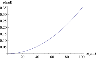
Figure 1: Phase difference $\delta$ as a function of $z$. Here $z$ and $z_{0}$ are the distances of the trajectories of the two atoms to the plate respectively, with parameters $z_{0}=1~{}{\rm\mu m}$, $\omega_{0}=3\times 10^{9}\,{\rm Hz}$, $\gamma_{0}/\omega_{0}=10^{-6}$, and $\theta=\pi/2$.

- (1) W. E. Lamb, Jr. and R. C. Retherford, Phys. Rev. 72, 241 (1947); H. A. Bethe, Phys. Rev. 72, 339 (1947).
- (2) H. B. G. Casimir, Proc. K. Ned. Akad. Wet. 51, 793 (1948).
- (3) H. B. G. Casimir and D. Polder, Phys. Rev. 73, 360 (1948).
- (4) G. L. Klimchitskaya, U. Mohideen, V. M. Mostepanenko, Rev. Mod. Phys. 81, 1827 (2009).
- (5) H. Yu and L. H. Ford, Phys. Rev. D 60, 084023 (1999); H. Yu and L. H. Ford, Phys. Lett. B 496, 107 (2000); H. Yu and P. X. Wu, Phys. Rev. D 68, 084019 (2003); H. Yu, N. F. Svaiter and L. H. Ford, Phys. Rev. D 80, 124019 (2009).
- (6) H. Yu and L. H. Ford, Phys. Rev. D 70, 065009 (2004); H. Yu and J. Chen, Phys. Rev. D 70 125006 (2004); H. Yu, X. Fu and P. Wu, J. Phys. A: Math. Theor. 41, 335402 (2008); H. Yu, J. Chen and P. Wu, JHEP 02, 058 (2006).
- (7) M. Brune et al., Phys. Rev. Lett. 72, 3339 (1994); M. Marrocco, M. Weidinger, R. T. Sang, and H. Walther, Phys. Rev. Lett. 81, 5784 (1998).
- (8) A.H. Safavi-Naeini et al, Phys. Rev. Lett. 108, 033602 (2012).
- (9) M. V. Berry, Proc. R. Soc. Lond. A 392, 45 (1984).
- (10) Geometric Phases in Physics, edited by A. Shapere and F.Wilczek (World Scientific, Singapore, 1989).
- (11) J. A. Jones, V. Vedral, A. Ekert, and G. Castagnoli, Nature 403, 869 (2000).
- (12) A. Uhlmann, Rep. Math. Phys. 24, 229 (1986).
- (13) E. Sjöqvist, A. K. Pati, A. Ekert, J. S. Anandan, M. Ericsson, D. K. L. Oi, and V. Vedral, Phys. Rev. Lett. 85, 2845 (2000).
- (14) K. Singh, D. M. Tong, K. Basu, J. L. Chen, and J. F. Du, Phys. Rev. A 67, 032106 (2003).
- (15) D. M. Tong, E. Sjöqvist, L. C. Kwek, and C. H. Oh, Phys. Rev. Lett. 93, 080405 (2004).
- (16) Z. S. Wang, L. C. Lwek, C. H. Lai, and C. H. Oh, Europhys. Lett. 74, 958 (2006).
- (17) A. Carollo, I. Fuentes-Guridi, M. F. Santos, and V. Vedral, Phys. Rev. Lett. 90, 160402 (2003); ibid. 92, 020402 (2004).
- (18) A. T. Rezakhani and P. Zanardi, Phys. Rev. A 73, 052117 (2006).
- (19) F. C. Lombardo and P. I. Villar, Phys. Rev. A 74, 042311 (2006).
- (20) J. J Chen, J. H. An, Q. J. Tong, H. G. Luo, and C. H. Oh, Phys. Rev. A 81, 022120 (2010).
- (21) K.-P. Marzlin, S. Ghose, and B. C. Sanders, Phys. Rev. Lett. 93, 260402 (2004).
- (22) J. Du, P. Zou, M. Shi, L. C. Kwek, J. W. Pan, C. H. Oh, A. Ekert, D. K. L. Oi, and M. Ericsson, Phys. Rev. Lett. 91, 100403 (2003).
- (23) M. Ericsson, D. Achilles, J. T. Barreiro, D. Branning, N. A. Peters, and P. G. Kwiat, Phys. Rev. Lett. 94, 050401 (2005).
- (24) F. M. Cucchietti, J.-F. Zhang, F. C. Lombardo, P. I. Villar, and R. Laflamme, Phys. Rev. Lett. 105, 240406 (2010).
- (25) E. Martin-Martinez, I. Fuentes and R. B. Mann, Phys. Rev. Lett. 107, 131301 (2011).
- (26) J. Hu and H. Yu, Phys. Rev. A 85, 032105 (2012).
- (27) G. Compagno, R. Passante, and F. Persico, Atom-Field Interactions and Dressed Atoms (Cambridge University Press, Cambridge, England, 1995).
- (28) S. Takagi, Prog. Theor. Phys. Suppl. 88, 1 (1986).
- (29) C. J. Bordé, J. Sharma, P. Tourrenc, and T. Damour, J. Phys. (Paris) 44, L983 (1983)
- (30) F. Benatti and R. Floreanini , Phys. Rev. A 70, 012112 (2004).
- (31) H. Yu and J. Zhang, Phys. Rev. D 77, 024031 (2008).
- (32) H. Yu, Phys. Rev. Lett. 106, 061101 (2011).
- (33) V. Gorini, A. Kossakowski, and E. C. G. Surdarshan, J. Math. Phys. 17, 821 (1976); G. Lindblad, Commun. Math. Phys. 48, 119 (1976).
- (34) F. Benatti and R. Floreanini, J. Opt. B 7, S429 (2005).
- (35) F. Benatti, R. Floreanini and M. Piani, Phys. Rev. Lett. 91, 070402 (2003).
- (36) J. M. Raimond, M. Brune, and S. Haroche, Rev. Mod. Phys. 73, 565 (2001); M. O. Scully, V.V. Kocharovsky, A. Belyanin, E. Fry, and F. Capasso, Phys. Rev. Lett. 91, 243004 (2003).
- (37) R. R. Chance, A. Prock, and R. Silbey, J. Chem. Phys. 62, 2245 (1975).
- (38) M. S. Yeung and T. K. Gustafson, Phys. Rev. A 54, 5227 (1996).
- (39) E. Sjöqvist, Physics 1, 35 (2008).