Coupling mechanism between microscopic two-level system and superconducting qubits

Abstract

We propose a scheme to clarify the coupling nature between superconducting Josephson qubits and microscopic two-level systems. Although dominant interests of studying two-level systems were in phase qubits previously, we find that the sensitivity of the generally used spectral method in phase qubits is not sufficient to evaluate the exact form of the coupling. On the contrary, our numerical calculation shows that the coupling strength changes remarkably with the flux bias for a flux qubit, providing a useful tool to investigate the coupling mechanism between the two-level systems and qubits.

Recent progress on superconducting qubits suggested that superconducting Josephson circuits are promising candidates for practical quantum computating Makhlin01 ; Clarke08 ; Neeley10 ; DiCarlo10 ; Sun10a . However, extensive works are needed to understand the decoherence mechanism hence increase the decoherence time of these macroscopic quantum systems. For instance, microscopic defects are ubiquitous in solid state devices. Each of these defects may behavior empirically as a quantum two-level-system (TLS) with characteristic frequency ranging about several gigahertz. The anticrossings resulting from the resonance between the TLSs and qubit were observed in the spectra of phase qubit Simmonds04 ; Sun10b , flux qubit Plourde05 , and charge qubit Schreier08 . Experiments have shown that TLSs not only shorten the decoherence time Cooper04 , but also reduce the visibility of Rabi oscillation of the qubit, limiting the fedelity of the quantum gate. Moreover, an ensemble of TLSs with various characteristic frequencies may produce low frequency $1/f$ noise Shnirman05 . Therefore, it is imperative to understand the microscopic coupling mechanism between TLS and superconducting qubits.

Unfortunately, it is nearly unattainable to directly probe a single TLS’s microscopic mechanism due to its microscopic nature. Nevertheless, utilizing qubit as a detector of TLS supplied an alternative method to extract useful information Cooper04 ; Martinis05 ; Yu08 . Based on the experimental results, three coupling models between TLS and superconducting qubit were suggested: critical current fluctuator Simmonds04 , electric dipole Martinis05 , and flux fluctuator Cole10 . Great effort has been put to determine which is the exact coupling mechanism Martinis05 ; Tian07 ; Kim08 ; Lupascedilcu09 ; Cole10 . Recently, it is suggested that one may clarify the coupling mechanism by investigating the longitudinal component of the interaction Hamiltonian Lupascedilcu09 ; Cole10 . Lupaşcu et al. have measured the flux qubit at symmetric double-well potential and only found transverse term Lupascedilcu09 . Furthermore, Cole et al. have theoretically shown that for different models, the coupling form between qubit and TLS changes remarkably. For the electric dipole model the coupling type is totally transverse, while for the other two models, besides the transverse, a weak longitudinal coupling exists Cole10 . However, their experiments in a flux-biased phase qubit is unable to determine the coupling type, because the observed longitudinal coupling strength is too small to discriminate it from the experimental uncertainty. Therefore, two questions come out from their works. One is whether we have to consider both transverse and longitudinal terms simultaneously for all superconducting qubits coupled with TLS. The other is whether the magnitude of the two terms depends on the coupling model thereby we can determine the exact coupling model by measuring the two terms. In this work, we have analyzed the interaction Hamiltonian of the three models. We found that the transverse and longitudinal terms vary for different types of superconducting qubits. For phase qubits the longitudinal coupling is always small thereby it is not a good system to probe the coupling form. However, the longitudinal term for flux qubits is comparable to the transverse term. In addition, for different coupling models the longitudinal term exhibits distinct flux bias dependencies, supplying a hopeful scheme to clarify the microscopic model of the TLS.
We start from a short review of the three models which are used to describe the microscopic nature of the coupling between TLS and qubits. Although they are also valid for flux qubits, we at first discuss them in a flux biased phase qubit for simplicity. The first model is critical current fluctuator. In this model, the microscopic TLS was assumed as a critical current fluctuator whose two states respond to two different critical currents of the Josephson junction Simmonds04 . The fluctuator could be considered as a ion moving between the left and right well in a double well potential. If $\hbar\varepsilon$ is the energy difference between the two position states, $\Delta$ is the tunneling matrix element, the interaction Hamiltonian can be written as Cole10

$$H_{I}=\upsilon_{i}\cos\hat{\phi}(\cos\theta\sigma_{T}^{x}+\sin\theta\sigma_{T}^{z})$$

with $\sigma_{T}^{x,z}$ being Pauli operators of TLS in its eigenenergy space. $\upsilon_{i}=-\frac{\delta I_{0}\phi_{0}}{2\pi},$ where $\delta I_{0}$ represents the difference of the critical currents for the ion populating the right and left well, $\phi_{0}$ is flux quantization. $\hat{\phi}$ is phase difference across the Josephson junction. $\theta$ denotes the relative orientation of the TLS’s configuration basis and eigenbasis, $\tan\theta=\varepsilon/\Delta$. Although in many literatures it is assumed $\theta=0$ Simmonds04 ; Ku05 , we would like to keeping the above formula which is more accurate and general.
The second model is the interaction of an electrical dipole with field Martinis05 . TLS has been modeled as an electric charge distribution that changed between the two states. In Ref. Martinis05 , each TLS was assumed as an electron of charge e at position R or L separated by a distance $d,$ resulting a dipole moment $\mu=ed$. The interaction Hamiltonian is given by

$$H_{I}=\overrightarrow{\mu}\cdot\overrightarrow{E}=\upsilon_{q}\hat{q}(\cos\theta\sigma_{T}^{x}+\sin\theta\sigma_{T}^{z})\cos\eta$$

where $\upsilon_{q}=\frac{2e^{2}d}{Cx}$. $x$ is the thickness of the junction. $\hat{q}$ represent the number of Cooper-pairs tunneled across the junction. $\eta$ denote the relative angle between electric dipole $\overrightarrow{\mu}$ and the electric field $\overrightarrow{E}$. The defination of $\theta$ is terminologically the same as that in the last model. However, $\varepsilon$ and $\Delta$ may depend on different physical variables. It is worth to note that the coupling term in this model is purely transverse no matter whether the double well of the TLS is symmetric Martinis05 ; Lupascedilcu09 ; Cole10 . This is a useful characteristic which offers a possibility to discriminate this coupling mechanism from others.
Another reasonable model for TLS is magnetic flux fluctuator. It has been found nearly three decades ago that the flux embraced by a rf-SQUID fluctuates with frequency lying in low frequency regime. The flux fluctuation is responsible for the dephasing of superconducting qubits. Recently, several experiments were carried out to probe the flux noise and found that the spectral density of the low frequency flux noise with the form $1/f$ Yoshihara06 ; Kakuyanagi07 ; Bialczak07 . Moreover, Shnirman et al. have shown that a collective of TLS’s with a natural distribution accounts for both high frequency and low frequency $1/f$ noise Shnirman05 . Therefore, a new explanation for TLS in superconducting phase qubit was proposed, suggesting that the states of the TLS may modulate the magnetic flux $\phi_{e}$ threading the superconducting loop Cole10 . The resulted coupling is on the variable $\hat{\phi}$ for the phase qubit. The interaction Hamiltonian can be written as

$$H_{I}=\upsilon_{\phi}\hat{\phi}(\cos\theta\sigma_{T}^{x}+\sin\theta\sigma_{T}^{z})$$

where $\upsilon_{\phi}=-\frac{\delta\phi_{e}}{L}(\frac{\phi_{0}}{2\pi})^{2}$. $\delta\phi_{e}$ is the difference of $\phi_{e}$ between the two configuration states of TLS. $\theta$ is defined the same as before, with $\varepsilon$ and $\Delta$ relying on different physical variables.

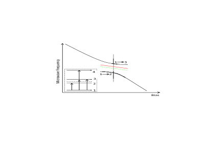
Figure 1: (Color online) Schematic diagram of the spectrum of a phase qubit resonantly coupled to a TLS. The green dashed line and red thin solid line represent the resonant peaks of the two-photon transition from state 1 to state 4 of the composite system without or with longitudinal coupling, respectively. Without longitudinal coupling, the two-photon spectrum locates at the exact middle of $1\rightarrow 2$ and $1\rightarrow 3$ one-photon transition lines. Note that with longitudinal coupling the two-photon spectrum can move up or down relative to the middle position, corresponding to positive or negetive sign of the longitudinal coupling. Here we chose positive sign as an example. Inset: the energy levels of the resonant qubit-TLS system.

The experimental investigation on the coupling mechanism is not very convincing. Recently, Cole $et$ $al.$ proposed a scheme to probe the coupling mechanism in a phase qubit Cole10 . Therein, whether the longitudinal coupling exists is a crucial clue to decide which model is true. The longitudinal coupling between resonant qubit-TLS leads to asymmetry of the two-photon transition spectrum relative to the one-photon transitions spectra: $\omega_{1\leftrightarrow 4}\neq\omega_{1\leftrightarrow 2}+\omega_{1\leftrightarrow 3}$ (1-4 denote the eigenstates of the coupled TLS-qubit system), as shown in Fig. 1. Therefore, one could experimentally resolve the coupling type of qubit-TLS system via spectral analysis. However, their experiment can not confirm the existence of the longitudinal coupling because its value is comparable to the measurement uncertainty. Hence, they could not reach a conclusion on the correct model. In our opinion, the key reason for the ambiguity is that the longitudinal is much smaller than the transverse coupling in all three models. To demonstrate this, we unify the interaction Hamiltonian

$$H_{I}=\upsilon_{k}\hat{O}(\cos\theta\sigma_{T}^{x}+\sin\theta\sigma_{T}^{z})$$

where $k=i,\phi,q$ and $\hat{O}=\cos\hat{\phi},\hat{\phi},\hat{q}$. Ignore the mixed terms such as $\sigma_{q}^{z}\sigma_{T}^{x}$, which have no effect on the spectrum of the system, we can write the interaction Hamiltonian in the eigenenergy basis

$$H_{I}=\upsilon_{k}(o_{x}^{k}\cos\theta\sigma_{q}^{x}\sigma_{T}^{x}+o_{z}^{k}\sin\theta\sigma_{q}^{z}\sigma_{T}^{z})$$

where the factors $o_{x,z}^{k}$ are given by

$$o_{x}^{k}=\frac{|\langle 1|\hat{O}|0\rangle+\langle 0|\hat{O}|1\rangle|}{2},\indent o_{z}^{k}=\frac{|\langle 1|\hat{O}|1\rangle-\langle 0|\hat{O}|0\rangle|}{2}$$

For the electric dipole model, $\hat{q}$ has no diagonal elements, $o_{z}^{q}=0$, so there is no longitudinal coupling in this case. Turning to the other two models, we numerically calculated $o_{x,z}^{i,\phi}$ as functions of flux bias using the parameters in Ref. Cole10 , shown in Fig. 2. It is found that $\frac{o_{z}^{i,\phi}}{o_{x}^{i,\phi}}<\frac{1}{6}$. Moreover, for $\phi_{e}>0.6$, the qubit can not work due to the large tunneling rate of the excite state; for $\phi_{e}<0.57$, $o_{z}^{i,\phi}$ is at least one order of magnitude smaller than $o_{x}^{i,\phi}$.The much smaller longitudinal coupling factor relative to the transverse one may be the main reason for which one can not verify the existence of the longitudinal interaction between qubit and TLS. Even worse, the corresponding coupling factors of the two models are roughly equal. This is easy to understand if we notice that in phase qubit, $\phi\simeq\frac{\pi}{2}$. We substitute $\phi$ with $\frac{\pi}{2}+\varphi$, where $\varphi$ is a small quantity,

$$\cos\phi=\cos(\frac{\pi}{2}+\varphi)=-\sin\varphi\simeq-\varphi=\frac{\pi}{2}-\phi$$

Figure 2: (Coler Online) Coupling factors of qubit- TLS interaction in phase qubitb for the critical current fluctuator and flux fluctuator models. The parameters of the phase qubit are: $C=850fF,L=720pH,I_{0}=984nA$. The green dash-dotted and cyan dashed line denote the transverse and longitudinal coupling factor $o_{x}^{i},o_{z}^{i}$ of the critical current fluctuator model respectively. The red solid and purple dotted line denote $o_{x}^{\phi},o_{z}^{\phi}$ of the flux fluctuator model respectively.

Taking $\cos\phi\simeq\frac{\pi}{2}-\phi$ into the coupling factors expressions, we can obtain: $o_{x}^{i}\simeq o_{x}^{\phi}$, $o_{z}^{i}\simeq o_{z}^{\phi}$. Therefore, for phase qubits, the longitudinal coupling is not sensitive to the coupling mechanism. Then, it is difficult to clarify the coupling nature between TLS and phase qubit . Although one may argue that the TLS parameter $\theta$ has a crucial effect on the longitudinal coupling magnitude, unfortunately, till now, people are unable to control the angle $\theta$ due to the poor knowledge of TLS.

Instead of phase qubit, we find that flux qubit is a possible system to reveal the coupling nature of TLS and qubits. We start from a flux qubit which consists of a superconducting loop interrupted by three Josephson junctions Orlando99 . Two junctions are the same and the other one is $\alpha$ times smaller than them. If we assume that the large junctions have a critical current $I_{0}$ and a capacitance $C$, then the critical current and capacitance of the small junction are $\alpha I_{0}$ and $\alpha C,$ respectively. The Hamiltonian of the circuit is Orlando99

$$H_{q} = 4E_{c}{\hat{n}_{1}}^{2}-E_{J}\cos{\hat{\phi}_{1}}+4E_{c}{\hat{n}_{2}}^{2}-E_{J}\cos{\hat{\phi}_{2}}+\frac{4E_{c}}{\alpha}{\hat{n}_{3}}^{2}$$ (1)

$$-\alpha E_{J}\cos{\hat{\phi}_{3}}+E_{J}(2+\alpha)$$

where $E_{c}=\frac{e^{2}}{2C}$, $E_{J}=I_{0}\phi_{0}/2\pi$. $\hat{\phi}_{i}\;(i=1,2,3)$ is the phase difference across each junction, and its conjugate variable $\hat{n}_{i}$ is the number of Cooper pair through each junction. If the external magnetic flux $\phi_{ext}=f\phi_{0}$, using the flux quantization condition, we get $\hat{\phi}_{3}=2\pi f+\hat{\phi}_{1}-\hat{\phi}_{2}$. Transforming the coordinates $\hat{\phi}_{1}$, $\hat{\phi}_{2}$ to the sum and the difference of the phases, $\hat{\phi}_{p}=(\hat{\phi}_{1}+\hat{\phi}_{2})/2,\,\hat{\phi}_{m}=(\hat{\phi}_{1}-\hat{\phi}_{2})/2$, $H_{q}$ is reduced to

$$H_{q} = E_{p}{\hat{n}_{p}}^{2}+E_{m}{\hat{n}_{m}}^{2}-2E_{J}\cos{\hat{\phi}_{p}}\cos{\hat{\phi}_{m}}+E_{J}(2+\alpha)$$

$$-\alpha E_{J}\cos(2\pi f+2\hat{\phi}_{m}))$$

where $E_{p}=2E_{c},\,\hat{n}_{p}=-i\frac{\partial}{\partial\phi_{p}}$, $E_{m}=E_{p}/(1+2\alpha),\,\hat{n}_{m}=-i\frac{\partial}{\partial\phi_{m}}$. We have calculated the lowest three energy levels near $f=0.5$ , with typically chosen parameters $E_{J}/E_{c}=40$, $\alpha=0.68$. In the region $0.49<f<0.51$, the energy difference between the lowest two levels (qubit) is much smaller than that between the upper two levels, showing a very good nonlinearity which enables the spectroscopic experiment will not involve the third level of the qubit.
In the three-junction flux qubit, each junction has the possibility of containing TLS. Even though, we can prove numerically that the location of the TLS in different junctions would not affect our results qualitatively. Therefore, we consider that the TLS is in the small junction without losing generality. For electric dipole model, the interaction term is

$$H_{I} = \vec{\mu}\cdot\vec{E}$$

$$= \frac{de}{x}\hat{V}(\cos\theta\sigma_{T}^{x}+\sin\theta\sigma_{T}^{z})\cos\eta$$

$$= \frac{de}{x}\frac{\phi_{0}}{2\pi}2\dot{\hat{\phi}}_{m}(\cos\theta\sigma_{T}^{x}+\sin\theta\sigma_{T}^{z})\cos\eta$$

Using Heisenberg equation $\dot{\hat{\phi}}_{m}=\frac{1}{i\hbar}[\hat{\phi}_{m},H_{q}]$, we obtain

$$H_{I}=\frac{\hbar\omega_{q}d\langle 0|\hat{\phi}_{m}|1\rangle}{x}\cos\eta\cos\theta\cdot\sigma_{q}^{x}\sigma_{T}^{x}$$ (2)

where $\hbar\omega_{q}$ is the eigenenergy of the flux qubit. Obviously, similar to that in phase qubit the longitudinal coupling is zero.

For the other models, following the same procedures used in the phase qubit, we can straightforwardly write out the interaction Hamiltonians.
Critical current model:

$$H_{I} = -\frac{\alpha\phi_{0}\delta I_{0}}{2\pi}\cos(2\pi f+2\hat{\phi}_{m})(\cos\theta\sigma_{T}^{x}+\sin\theta\sigma_{T}^{z})$$ (3)

$$= -\frac{\alpha\phi_{0}\delta I_{0}}{2\pi}(o_{x}^{i}\cos\theta\sigma_{q}^{x}\sigma_{T}^{x}+o_{z}^{i}\sin\theta\sigma_{q}^{z}\sigma_{T}^{z})$$

$$o_{x}^{i} = \frac{|\langle 1|\cos(2\pi f+2\hat{\phi}_{m})|0\rangle+\langle 0|\cos(2\pi f+2\hat{\phi}_{m})|1\rangle|}{2}$$

$$o_{z}^{i} = \frac{|\langle 1|\cos(2\pi f+2\hat{\phi}_{m})|1\rangle-\langle 0|\cos(2\pi f+2\hat{\phi}_{m})|0\rangle|}{2}$$

Magnetic flux fluctuator model

$$H_{I} = 2\pi\alpha E_{J}\delta\phi_{e}\sin(2\pi f+2\hat{\phi}_{m})(\cos\theta\sigma_{T}^{x}+\sin\theta\sigma_{T}^{z})$$ (4)

$$= 2\pi\alpha E_{J}\delta\phi_{e}(o_{x}^{\phi}\cos\theta\sigma_{q}^{x}\sigma_{T}^{x}+o_{z}^{\phi}\sin\theta\sigma_{q}^{z}\sigma_{T}^{z})$$

$$o_{x}^{\phi} = \frac{|\langle 1|\sin(2\pi f+2\hat{\phi}_{m})|0\rangle+\langle 0|\sin(2\pi f+2\hat{\phi}_{m})|1\rangle|}{2}$$

$$o_{z}^{\phi} = \frac{|\langle 1|\sin(2\pi f+2\hat{\phi}_{m})|1\rangle-\langle 0|\sin(2\pi f+2\hat{\phi}_{m})|0\rangle|}{2}$$

Figure 3: (Color online) Transverse (solid line) and longitudinal (dashed line) coupling factors for critical current fluctuator model.

Figure 4: (Color online) Transverse (solid line) and longitudinal (dashed line) coupling factors for flux fluctuator model.

Now we compare the magnitudes of the transverse and longitudinal couplings. As discussed before, currently it is impossible to change the orientation of the TLS basis, we focus on the factors $o_{x,z}^{i,\phi}$. Using the same parameters as above ($E_{J}/E_{c}=40$, $\alpha=0.68$), we have numerically calculated $o_{x,z}^{i,\phi}$ as functions of $f,$ shown in Fig. 3 and 4. When $f$ varies from 0.5 to 0.51, $o_{x,z}^{i,\phi}$ exhibit remarkable changes with totally different trends. For critical current fluctuator model (Fig. 3), the transverse coupling factor $o_{x}^{i}$ is zero at the degenerate point $f=0.5$ while the longitudinal factor reaches the maximum. Then, away from $f=0.5$, the transverse factor increases monotonically while the longitudinal one decreases gradually. At $f=0.51$, the transverse factor becomes much larger than the longitudinal one. In recent experiments Lupascedilcu09 , the splitting resulted from transverse coupling is observed at the degeneracy point of a flux qubit. In addition, no longitudinal coupling is observed at $f=0.5$. These behaviors disagree with the predictions of the critical current fluctuator model, indicating that the critical current fluctuation is not the dominate mechanism of the qubit-TLS coupling.
For the flux fluctuator model, the trends are totally converse (Fig. 4). The transverse factor reaches maximum at the degenerate point while the longitudinal magnitude vanishes, indicating that the coupling is pure transverse at this point. However, the electric dipole model predicts similar pure transverse coupling [see Eq. (2)]. we can not discriminate the flux fluctuator and the electric dipole model at the degenerate point. When we tune the flux bias away from $f=0.5$, the transverse factor decreases and the longitudinal one increases gradually. At $f=0.51$, the longitudinal factor is larger than $1.5$ times of the transverse one. Therefore, the flux fluctuator model contains both transverse and longitudinal coupling but in the electric dipole model only transverse interaction exists. We can clarify the microscopic mechanism of TLS by studying the coupling term of TLS-flux qubit interaction in a flux qubit biased away from the degenerate point. In practical, TLSs have been observed in three-junction flux qubits biased away from the degenerate point Plourde05 , suggesting that this spectral method is completely feasible with the current technique.
In summary, we have calculated the qubit-TLS coupling factors of both transverse and longitudinal terms under three microscopic models. It is found that for phase qubits the longitudinal coupling is difficult to observe because it is always much smaller than the transverse coupling. Then, we show that in three-junction flux qubit the relative magnitude of the transverse and longitudinal coupling factors are largely model-dependent and very sensitive to the external flux bias. We propose that these features can be used to clarify the microscopic model of TLS.

This work was supported in part by MOST (2011CB922104, 2011CBA00200), NSFC (91021003, 10725415), and the Natural Science Foundation of Jiangsu Province (BK2010012).

References

- (1) Y. Makhlin et al., Rev. Mod. Phys. 73, 357 (2001).
- (2) J. Clarke and F. K. Wilhelm, Nature 453, 1031 (2008).
- (3) M. Neeley, et al., Nature 467, 570 (2010).
- (4) L. DiCarlo et al., Nature 467, 574 (2010).
- (5) G. Sun et al., Nat Commun 1, 51 (2010).
- (6) R.W. Simmonds et al., Phys. Rev. Lett. 93, 077003 (2004).
- (7) G. Sun et al., Phys. Rev. B 82, 132501 (2010).
- (8) B. L. T. Plourde et al., Phys. Rev. B 72, 060506 (2005).
- (9) J. A. Schreier et al., Phys. Rev. B 77, 180502 (2008).
- (10) K. B. Cooper et al., Phys. Rev. Lett. 93, 180401 (2004).
- (11) A. Shnirman, et al., Phys. Rev. Lett. 94, 127002 (2005).
- (12) J. M. Martinis et al., Phys. Rev. Lett. 95, 210503 (2005).
- (13) Y. Yu et al., Phys. Rev. Lett. 101, 157001 (2008).
- (14) J. H. Cole et al., Appl. Phys. Lett. 97, 252501 (2010).
- (15) L. Tian, Phys. Rev. Lett. 98, 153602 (2007).
- (16) Z. Kim et al., Phys. Rev. B 78, 144506 (2008).
- (17) A. Lupaşcu et al., Phys. Rev. B 80, 172506 (2009).
- (18) L.-C. Ku and C. C. Yu, Physical Review B 72, 024526 (2005).
- (19) F. Yoshihara et al., Phys. Rev. Lett. 97, 167001 (2006).
- (20) K. Kakuyanagi et al., Phys. Rev. Lett.98, 047004 (2007).
- (21) R. C. Bialczak et al., Phys. Rev. Lett. 99, 187006 (2007).
- (22) T. P. Orlando et al., Phys Rev B 60, 15398 (1999).