Surface subgroups from linear programming

Abstract.

We show that certain classes of graphs of free groups contain surface subgroups, including groups with positive $b_{2}$ obtained by doubling free groups along collections of subgroups, and groups obtained by “random” ascending HNN extensions of free groups. A special case is the HNN extension associated to the endomorphism of a rank 2 free group sending $a$ to $ab$ and $b$ to $ba$; this example (and the random examples) answer in the negative well-known questions of Sapir. We further show that the unit ball in the Gromov norm (in dimension 2) of a double of a free group along a collection of subgroups is a finite-sided rational polyhedron, and that every rational class is virtually represented by an extremal surface subgroup. These results are obtained by a mixture of combinatorial, geometric, and linear programming techniques.

1. Introduction

1.1. Gromov’s surface subgroup question

The following well-known question is usually attributed to Gromov:

Question 1.1 (Gromov).

Let $G$ be a one-ended hyperbolic group. Does $G$ contain the fundamental group of a closed surface with $\chi<0$?

Hereafter we abbreviate “fundamental group of a closed surface with $\chi<0$” to “surface group”, so that this question asks whether every one-ended hyperbolic group contains a surface subgroup. This question is wide open in general, but a positive answer is known in certain special cases, including:

1. Coxeter groups (Gordon–Long–Reid [14]);

2. Graphs of free groups with cyclic edge groups and $b_{2}>0$ (Calegari [4]);

3. Fundamental groups of hyperbolic $3$-manifolds (Kahn–Markovic [19]);

4. Certain doubles of free groups (Gordon–Wilton, Kim–Wilton, Kim–Oum [15, 21, 20]);

(this list is not exhaustive).

The main goal of this paper is to describe how linear programming may be used to settle the question of the existence of surface subgroups in certain graphs of free groups, either by giving a powerful computational tool to find surface subgroups in specific groups, or by reducing the analysis of this question in infinite families of groups to a finite (tractable) calculation. There are many reasons why the case of graphs of free groups is critical for Gromov’s question, but we do not go into this here, taking the interest of Gromov’s question in this subclass of groups to be self-evident.

1.2. Statement of results

We are able to prove the existence of surface subgroups in the following groups:

1. A group $G$ with $b_{2}>0$ obtained by doubling a free group $F$ along a finite collection of finitely generated subgroups $F_{i}$;

2. A group $G$ obtained as an HNN extension $F*_{\phi}$ where $F$ is a free group of fixed rank and $\phi$ is a random endomorphism;

3. “Sapir’s group” $C=F*_{\phi}$ for $F=\langle a,b\rangle$ and $\phi:a\to ab,b\to ba$.

The sense in which this constitutes a significant advance over the results and methods in [4, 21, 20] is that the edge groups are free groups of arbitrary rank, whereas in the cited papers the edge groups were required to be cyclic.

Bullet (1) above is implied by a stronger result about the Gromov norm on $H_{2}$ of the double of $F$ along the $F_{i}$, which we discuss in § 1.3. Bullet (3) is reasonably self-explanatory. A precise statement of bullet (2) is:

Random $f$-folded Surface Theorem 4.16.

Let $k\geq 2$ be fixed, and let $F$ be a free group of rank $k$. Let $\phi$ be a random endomorphism of $F$ of length $n$. Then the probability that $F*_{\phi}$ contains an essential surface subgroup is at least $1-O(C^{-n^{c}})$ for some $C>1$ and $c>0$.

Here a random endomorphism of length $n$ is one that takes the generators to reduced words of length $n$ chosen independently and randomly with the uniform distribution. We became interested in surface subgroups of HNN extensions of free groups after discussions with Mark Sapir, who conjectured that the subgroup $C$ does not contain a surface subgroup, and thought it was unlikely that many HNN extensions should contain surface subgroups (other than $\mathbb{Z}^{2}$ subgroups for endomorphisms fixing a nontrivial conjugacy class). See also [11] and [25]. Therefore it seems safe to say that the Random $f$-folded Surface Theorem is in many ways very unexpected.

1.3. Gromov norm

If $X$ is a $K(\pi,1)$, the Gromov norm of a class $\alpha\in H_{2}(X;\mathbb{Q})$, denoted $\|\alpha\|$ is the infimum of $-2\chi(S)/n$ over all closed oriented surfaces $S$ without sphere components, and all positive integers $n$, so that there is a map $f:S\to X$ with $f_{*}[S]=n\alpha$. If $G$ is a group, define the Gromov norm on $H_{2}(G;\mathbb{Q})$ by identifying this space with $H_{2}(X;\mathbb{Q})$ for $X$ a $K(G,1)$. The function $\|\cdot\|$ extends by continuity to $H_{2}(X;\mathbb{R})$, where (despite its name) it defines a pseudo-norm in general.

There is a relative version of Gromov norm for surfaces with boundary, and classes in $H_{2}(X,Y)$ for subspaces $Y\subset X$, and when $H_{2}(X)=0$ this relative Gromov norm is equivalent (up to a factor of 4) to the stable commutator length norm, as defined in [5], Ch. 2 (also see the start of § 3). There are equivalent definitions for pairs $G,\{G_{i}\}$ where $G$ is a group and $\{G_{i}\}$ is a family of conjugacy classes of subgroups of $G$.

In § 2 and § 3 we develop tools to compute stable commutator length in free groups relative to families of finitely generated subgroups, and show (Theorem 2.15) that the unit balls in the norm are finite sided rational polyhedra. By a doubling argument, we obtain a similar theorem for Gromov norms of groups obtained from free groups by doubling along a collection of subgroups:

Double Norm Theorem 3.6.

Let $F$ be a finitely generated free group, and let $F_{i}$ be a finite collection of conjugacy classes of finitely generated subgroups of $F$. Let $G$ be obtained by doubling $F$ along the $F_{i}$. Then the unit ball in the Gromov norm on $H_{2}(G)$ is a finite sided rational polyhedron, and each rational class is projectively represented by an extremal surface.

Since extremal surfaces are necessarily $\pi_{1}$-injective, this shows that a group $G$ as in the theorem contains a surface subgroup when $H_{2}(G)$ is nontrivial.

1.4. Unity of methods

The Double Norm Theorem and the Random $f$-folded Surface Theorem are logically independent, and the certificates for $\pi_{1}$-injectivity of the surface subgroups they promise are quite different. However, the surfaces in either case are constructed combinatorially from pieces obtained by solving a rational linear programming problem; and the nature of the representation of the surfaces by vectors, and the tools used to set up the linear programming problems, are very similar. Thus there is a deeper unity of methods underlying the two theorems, beyond the similarity that both promise surface subgroups in certain graphs of free groups.

1.5. Acknowledgments

We would like to thank Sang-Hyun Kim, Tim Susse and Henry Wilton for helpful conversations about the material in this paper. Danny Calegari was supported by NSF grant DMS 1005246, and Alden Walker was supported by NSF grant DMS 1203888.

2. Traintrack Rationality Theorem

2.1. Graphs and traintracks

We recall some standard definitions from the theory of graphs, traintracks and immersions, and their connection to free groups and morphisms between them. See e.g. [2] for background and more details.

We fix a free group $F$ of finite rank and a free generating set for $F$, and realize $F$ as the fundamental group of a rose $R$, identifying the generators of $F$ with the (oriented) edges of $R$. If $X$ is a graph, an immersion $X\to R$ is a locally injective simplicial map taking edges to edges. Every nontrivial conjugacy class in $F$ is represented by an immersed loop in $R$, unique up to reparameterization of the domain (which is an oriented circle).

Definition 2.1.

Let $T$ be a graph. A turn is an ordered pair of distinct oriented edges incident to a vertex of $T$, the first element incoming and the second outgoing. If $e_{1}$ is the incoming edge and $e_{2}$ the outgoing edge, we denote the turn $e_{1}\to e_{2}$.

Thus, a turn is the same thing as the germ at a vertex of an oriented immersed path in $T$.

Definition 2.2.

A traintrack is a graph $T$ together with a subset of the turns at each vertex which are called admissible turns. If $L$ is an oriented 1-manifold, an immersion $L\to T$ is admissible if the germ of $L$ is admissible at every vertex of $T$. A traintrack immersion is a simplicial map $T\to R$ taking edges to edges, which is locally injective on each admissible turn.

Thus if $L\to T$ is admissible, and $T\to R$ is a traintrack immersion, then $L\to R$ is an immersion.

If $X$ is a graph and we fix a simplicial map $X\to R$, we label the oriented edges of $X$ by the generators of $F$ corresponding to the edges that they map to. Any oriented 1-manifold mapping $L\to X$ pulls back these labels so that each component of $L$ is labeled by a cyclic word in $F$. If $T$ is a traintrack and $T\to R$ is a traintrack immersion and $L\to T$ is admissible, then the labels on the components of $L$ are cyclically reduced words.

Conversely, suppose we are given a finite set $\Gamma$ of nontrivial conjugacy classes in $F$. We let $L$ be an oriented simplicial 1-manifold with one component for each element of $\Gamma$, and each component labeled by the cyclically reduced word representing the given conjugacy class. There is a unique immersion $L\to R$ compatible with the labels. We say that $L$ is carried by a traintrack immersion $T\to R$ if $L\to R$ factors through an admissible map $L\to T$. See Figure 1.

2pt $b$ at 4 45 $c$ at 1 9 $a$ at 33 2 $b$ at 40 42

$A$ at 61 46 $A$ at 51 18 $c$ at 67 0 $c$ at 92 2 $a$ at 103 25 $b$ at 91 47

$b$ at 145 37 $A$ at 174 26 $b$ at 214 0 $a$ at 217 47 $c$ at 262 26 $c$ at 293 35

$a$ at 340 5 $b$ at 410 11 $c$ at 372 58

Figure 1. The pair of loops $L$ maps to the rose $R$, and this map factors through an admissible map to the traintrack $T$, so $L$ is carried by $T$.

Definition 2.3.

If $T$ is a traintrack, a weight $w$ is an assignment of real numbers to the admissible turns in such a way that for each oriented edge $e$, the sum of numbers associated to turns involving $e$ at one vertex is equal to the sum at the other.

The space of weights on $T$, denoted $W(T)$, is a real vector space defined over $\mathbb{Q}$. Weights can be non-negative, integral, and so on. The space of non-negative weights is a convex rational cone $W^{+}(T)$.

A carrying map $L\to T$ determines a function from admissible turns to non-negative integers, where the number assigned to a turn is the number of times that $L$ makes such a turn when it passes through the given vertex. We denote this function $w(L)$.

Lemma 2.4.

The set of functions $w(L)$ over all carrying maps $L\to T$ is precisely the set of integer weights in $W^{+}(T)$.

Proof.

Each edge of $L$ contributes $1/2$ to the value of $w(L)$ on the turns at its vertices, so $w(L)\in W^{+}(T)$.

Conversely, let $w$ be a non-negative integer weight in $W^{+}(T)$. For each turn $e\to e^{\prime}$ with weight $n$, take $n$ disjoint intervals made by gluing the front half of $e$ to the back half of $e^{\prime}$, and glue these oriented intervals together (over all turns) compatibly with how they immerse in $T$ to produce $L$. The defining property of a weight says that this gluing can be done, and $w(L)=w$. ∎

Note that $w(L)$ does not determine the topology of $L$ (i.e. the number of components). But it does determine the image of $L$ in $H_{1}(F)$ under $L\to R$. Thus we obtain a homomorphism $h:W(T)\to H_{1}(F)$, defined over $\mathbb{Q}$, so that the image of $[L]$ in $H_{1}(R)=H_{1}(F)$ is $h(w(L))$.

2.2. Fatgraphs and scl

For an introduction to fatgraphs, see [22].

Definition 2.5.

A fatgraph is a graph $X$ together with a choice of cyclic ordering of the edges incident to each vertex. A fatgraph admits a canonical fattening to a compact oriented surface $S(X)$ in such a way that $X$ sits inside $S(X)$ as a spine to which $S(X)$ deformation retracts. The boundary $\partial S(X)$ is an oriented 1-manifold, which comes with a canonical map $\partial S(X)\to X$ which is the restriction of the deformation retraction, and is an immersion unless $X$ has 1-valent vertices.

A fatgraph over $F$ is a fatgraph $X$ together with a simplicial map of the underlying graph $X\to R$. It is reduced if the composition $\partial S(X)\to X\to R$ is an immersion. See Figure 2.

2pt $a$ at 13 58 $A$ at 23 41 $c$ at 31 13 $C$ at 36 -4 $b$ at 72 -4 $B$ at 78 16 $A$ at 84 25 $a$ at 84 43 $b$ at 121 24 $B$ at 122 44 $c$ at 160 5 $C$ at 161 23 $b$ at 198 23 $B$ at 199 44 $a$ at 161 63 $A$ at 160 44 $a$ at 278 11 $b$ at 340 9 $c$ at 308 67

Figure 2. This fatgraph map $X\to R$ is an immersion, but the fatgraph is not reduced because the boundary is not reduced.

If $X\to R$ is a fatgraph over $F$ without 1-valent vertices, and if the underlying map of graphs $X\to R$ is an immersion, the fatgraph is reduced. The converse is true if $X$ is 3-valent, but not in general otherwise. All the fatgraphs we consider in this paper will be immersed. Moreover, throughout § 2 they will also be reduced. However we need to consider unreduced fatgraphs in § 4.4.

Now, let $f:L\to R$ be an oriented 1-manifold mapping to $R$ by an immersion; equivalently, $L$ and $f$ are determined by the data of a collection $\Gamma$ of nontrivial conjugacy classes in $F$.

Definition 2.6.

An admissible surface for $f:L\to R$ is a compact oriented surface $S$ together with a map $g:S\to R$ and an oriented covering map $h:\partial S\to L$ so that $f\circ h=g|\partial S$.

We denote the degree of the covering map $h:\partial S\to L$ by $n(S)$. We say that ad admissible surface $S$ is efficient if no component of $S$ is a sphere, and if every component of $S$ is geometrically incompressible; i.e. if there is no essential embedded loop in $S$ mapping to a null-homotopic loop in $R$. Any admissible surface can be replaced by an efficient one, by throwing away sphere components and repeatedly performing compressions. Note that since by hypothesis every component of $L$ maps to a nontrivial immersed loop in $R$, no component of $S$ is a disk, and therefore every component of $S$ has non-positive Euler characteristic.

The following proposition is essentially due to Culler [12] (see also [5] § 4.1) and lets us reduce the study of admissible surfaces to combinatorics:

Proposition 2.7.

Every efficient admissible surface for every oriented $f:L\to R$ is homotopic to a surface obtained by fattening a reduced fatgraph over $F$.

Definition 2.8.

Let $\Gamma$ be a finite collection of conjugacy classes in $F$ whose sum is homologically trivial (i.e. represents $0$ in $H_{1}(F)$). The stable commutator length of $\Gamma$, denoted $\textnormal{scl}(\Gamma)$, is defined to be the infimum

$$\textnormal{scl}(\Gamma)=\inf_{S}-\chi(S)/2n(S)$$

over all efficient admissible surfaces $S$ for $L$, where $f:L\to R$ represents $\Gamma$. A surface is extremal for $\Gamma$ if equality is achieved.

The main theorem of [6] says that extremal surfaces exist for any $\Gamma$. For more background and an introduction to the theory of stable commutator length, see [5] or [1].

2.3. Polygons

Let $X$ be a reduced fatgraph over $R$ with fattening $S(X)$ and oriented boundary $\partial S(X)$. There is a decomposition of $S(X)$ into polygons — canonical up to isotopy — where all vertices of each polygon are vertices on $\partial S(X)$, with one rectangle for each edge of $X$, and one $n$-gon for each $n$-valent vertex of $X$. Each $n$-gon with $n\geq 3$ may be further decomposed into $n-2$ triangles, without introducing new vertices; this decomposition is not canonical unless every vertex of $X$ is at most 3-valent. Thus, we decompose $S(X)$ into two kinds of polygons: rectangles and triangles. Note that $\chi(X)=\chi(S(X))=-\tau/2$ where $\tau$ is the number of triangles. See Figure 3.

2pt

Figure 3. A fatgraph $S(X)$ (left) can be cut into rectangles and polygons (center), and the polygons can be further cut into triangles (right).

The edges of the polygons could be boundary edges, which are edges of $\partial S(X)$, or internal edges, which are determined by ordered pairs of vertices of $\partial S(X)$. A polygon is determined by the cyclic list of its edges; thus, a rectangle has four edges which alternate between boundary edges and internal edges, while a triangle has three internal edges. Note that the edge labels on the two boundary edges of a rectangle have inverse labels. Summarizing: a rectangle piece is determined by the data of a pair of edges of $\partial S(X)$ with inverse labels, while a triangle is determined by the data of a cyclically ordered list of three vertices of $\partial S(X)$. In particular, there are finitely many polygon types (at most cubic in the length of $X$).

Now suppose that $\partial S(X)$ is carried by some immersed traintrack $T\to R$. Each rectangle determines a pair of edges of $\partial S(X)$ with inverse labels, which are mapped to a pair of oriented edges of $T$ with inverse labels. At each vertex, $\partial S(X)$ makes some admissible turn in $T$; we record the information of these admissible turns at the vertices. Similarly, each triangle determines a cyclically ordered list of vertices of $\partial S(X)$ which are mapped to a cyclically ordered list of admissible turns of $T$.

Definition 2.9.

Let $T\to R$ be an immersed traintrack. A triangle over $T$ is a cyclically ordered list of three admissible turns. A rectangle over $T$ is a cyclically ordered list of 4 admissible turns of the form $e_{1}\to e_{2}$, $e_{2}\to e_{3}$, $e_{4}\to e_{5}$, $e_{5}\to e_{6}$ where $e_{2}$ and $e_{5}$ have inverse labels. See Figure 4.

2pt

Figure 4. If a fatgraph boundary $\partial S(X)$ is carried by an immersed traintrack $T\to R$, then each vertex of each rectangle and triangle is associated with an admissible turn in $T$ (blue). As we cut $S(X)$ into rectangles and triangles, we record these admissible turns for each piece; using this information, we can reassemble the pieces into a fatgraph carried by $T$.

A rectangle over $T$ determines two ordered pairs $(e_{2}\to e_{3},e_{4}\to e_{5})$ and $(e_{5}\to e_{6},e_{1}\to e_{2})$ with notation as above; call these pairs the internal edges of the rectangle, while the edges $e_{2}$ and $e_{5}$ are the boundary edges. Similarly, call the three ordered pairs arising as the boundary of a triangle over $T$ the internal edges of the triangle.

Definition 2.10.

If $T\to R$ is an immersed traintrack, a polygon weight is an assignment of real numbers to triangles and rectangles in such a way that for every unordered pair of admissible turns, the number of times it appears as an internal edge with one ordering is the same as the number of times it appear as an internal edge with the other ordering.

The space of polygon weights on $T$, denoted $P(T)$, is a real vector space defined over $\mathbb{Q}$. The space of non-negative weights is a convex rational cone $P^{+}(T)$. By the discussion above, if $X$ is a reduced fatgraph over $R$ with fattening $S(X)$ and oriented boundary $\partial S(X)$ carried by $T$, then after decomposing $S(X)$ into rectangles and triangles, we obtain a vector $p(X)$ whose coefficients are the number of each kind of polygon over $T$ (note that $p(X)$ depends not just on $X$ but on the decomposition into triangles, although our notation obscures this).

Lemma 2.11.

Let $X$ be a reduced fatgraph over $R$ with fattening $S(X)$ and oriented boundary $\partial S(X)$ carried by $T$. Then $p(X)\in P^{+}(T)$.

Proof.

This is just the observation that the polygons into which $S(X)$ is decomposed are glued together in pairs along internal edges. ∎

Lemma 2.12.

There is a rational linear map $\partial:P^{+}(T)\to W^{+}(T)$ so that if $X$ is a fatgraph with $\partial S(X)$ carried by $T$, then $\partial p(X)=w(\partial S(X))$.

Proof.

The map $\partial$ takes each rectangle to the vector consisting of the 4 admissible turns appearing as vertices, each with weight $1/2$. Define $\partial$ to be zero on triangles, and extend by linearity. This map has the desired properties. ∎

Note that $\partial$ takes integer vectors to integer vectors (though we do not use this fact).

Lemma 2.13.

There is a rational linear map $-\chi:P^{+}(T)\to\mathbb{R}$ so that if $X$ is a fatgraph with $\partial S(X)$ carried by $T$, then $-\chi(p(X))=-\chi(S(X))$.

Proof.

Define $-\chi$ to be $1/2$ on every triangle, and $0$ on rectangles. ∎

Again, $-\chi$ takes integer vectors to integers.

Proposition 2.14.

For every non-negative integer weight $p$ in $P^{+}(T)$ there is some non-negative integer weight $p^{\prime}$ with $\partial p=\partial p^{\prime}$ and $-\chi(p)\geq-\chi(p^{\prime})$, and such that $p^{\prime}=p(X)$ for some fatgraph $X\to R$ with $\partial S(X)$ carried by $T$.

Proof.

An integral weight $p$ determines a collection of triangles and rectangles where the weight of each piece determines the number of copies. Polygons can be glued together along the same internal edge with opposite orderings; by the definition of a weight, this can be done to produce a surface $S$ without corners. The surface $S$ might contain some components without rectangles (i.e. consisting entirely of triangles); throw these pieces away. The surface $S$ might also contain some subsurface made entirely of triangles with nontrivial topology. Compress these surfaces down to disks, and triangulate the result without introducing new vertices on the boundary. The result is a new surface which by construction is of the form $S(X)$ for some fatgraph $X\to R$. The compression did not affect boundary edges, so $\partial p=\partial p^{\prime}$. Moreover, compression can only reduce the number of triangles used, so $-\chi(p)\geq-\chi(p^{\prime})$. This completes the proof. ∎

2.4. Traintrack Rationality Theorem

For $w\in W^{+}(T)$ rational and in the kernel of $h:W^{+}(T)\to H_{1}(F)$, we can define $\textnormal{scl}(w)$ to be the infimum of $\textnormal{scl}(\Gamma)/n$ for all homologically $\Gamma$ represented by an oriented 1-manifold $L$ carried by $T$ with $w(L)=nw$ for some $n$. The following Traintrack Rationality Theorem is the main theorem of this section.

Theorem 2.15 (Traintrack Rationality Theorem).

Let $T$ be a traintrack immersing to $R$, and let $B^{+}(T)$ denote the kernel of $h:W^{+}(T)\to H_{1}(F)$. The function scl extends continuously to $B^{+}(T)$ in a unique way, where it is convex and piecewise rational linear. For any rational $w\in B^{+}(T)$ there is some homologically trivial $\Gamma$ and a fatgraph $X$ over $F$ with $\partial S(X)$ representing $\Gamma$, in such a way that $\partial S(X)$ is carried by $T$ with $w(\partial S(X))=nw$ and $\textnormal{scl}(w)=-\chi(S(X))/2n$.

In particular, the surface $S(X)$ is extremal for $\partial S(X)$.

Proof.

Define $Q(w)=P^{+}(w)\cap\partial^{-1}(w)$; this is a convex linear polyhedron, and is rational if $w$ is rational. Define

$$\textnormal{scl}(w)=\inf_{q\in Q(w)}-\chi(q)/2$$

This is evidently convex and piecewise rational linear on $B^{+}(T)$. We show that it agrees with the definition of $\textnormal{scl}(w)$ already given when $w$ is rational, and that there is an extremal surface obtained from some fatgraph.

The infimum of $-\chi$ on $Q(w)$ is achieved on some nonempty subpolyhedron $E(w)$, which is convex in general, and rational if $w$ is rational. A nonempty rational polyhedron contains a rational point, and every rational $p\in E(w)$ can be rescaled to an integer point $np$, which is in $E(nw)$ by linearity of the maps and $-\chi$; and by Proposition 2.14, there is some fatgraph $X$ with $\partial S(X)$ carried by $T$ and with $w(\partial S(X))=nw$ and $-\chi(S(X))=-\chi(np)$.

Conversely, any efficient admissible surface $S$ with $\partial S$ carried by $T$ and with $w(\partial S)=mw$ for some $m$ can be obtained as $S=S(X)$ for some reduced fatgraph $X$ over $R$ by Proposition 2.7. Then any $p(X)$ satisfies $\partial p(X)=mw$, so $p(X)\in Q(mw)$. But then

$$-\chi(S(X))/2m=-\chi(p(X))/2m\geq-\chi(E(w))/2$$

Thus $\textnormal{scl}(w)=-\chi(E(w))/2$, and the surface constructed from $p$ above was extremal, as claimed. ∎

Example 2.16 (Verbal traintracks).

Fix a free group $F$ of rank $k$ and a free generating set, and fix a positive integer $\ell$. Define a traintrack $T_{\ell}$ whose oriented edges are the set of reduced words in $F$ of length $\ell-1$ and whose admissible turns are reduced words of length $\ell$, which we think of as an ordered pair of oriented edges consisting of the prefix and suffix of the given word of length $\ell-1$.

Let $W_{\ell}$ denote the weight space, and $W_{\ell}^{+}$ the non-negative weights as above. There is an involution $\epsilon$ on $W_{\ell}$, which takes $\sigma$ to $-\sigma^{-1}$, where $\sigma^{-1}$ denotes the inverse word to a reduced word $\sigma$. The natural inclusion $W_{\ell}^{+}\to W_{\ell}$ induces a surjection $W_{\ell}^{+}\to W_{\ell}/\epsilon$, and we obtain a rational linear (pseudo)-norm on $W_{\ell}/\epsilon$, where the norm $\|[w]\|$ of an equivalence class $[w]$ is the infimum of the $\textnormal{scl}(w)$ over all $w\in W_{\ell}^{+}$ mapping to $w$. The linear functions on $W_{\ell}/\epsilon$ are precisely real linear combinations of the homogeneous (big) counting quasimorphisms of length at most $\ell$ first introduced by Rhemtulla [24] and studied later by Brooks [3], Grigorchuk [16] and others. Thus we may use $W_{\ell}/\epsilon$ to get an explicit and complete set of linear relations between the homogeneous counting quasimorphisms supported on words of any bounded length. For more details, see [9], especially § 4–5.

3. Gromov Norm of doubles

We briefly introduce the Gromov norm on the homology of a space or group, and its relative variants.

Definition 3.1.

Let $X$ be a topological space. The Gromov (pseudo)-norm (also called the $L_{1}$ norm) of a homology class $\alpha\in H_{i}(X;\mathbb{R})$, denoted $\|\alpha\|$, is the infimum of $\sum|t_{i}|$ over all real singular $i$-cycles $\sum t_{i}\sigma_{i}$ representing $\alpha$. Similarly define a norm on relative classes $\alpha\in H_{i}(X,Y;\mathbb{R})$ for a subspace $Y\subset X$ from relative $i$-cycles.

If $G$ is a group, we can define the Gromov norm on $H_{*}(G)$ by identifying the group homology with $H_{*}(K(G,1))$.

Definition 3.2.

If $G_{i}$ is a family of conjugacy classes of subgroups of $G$, we can build a space $K$ as the mapping cylinder of $\coprod_{i}K(G_{i},1)\to K(G,1)$, and we define the Gromov norm on $H_{*}(G,\{G_{i}\})$ by identifying group homology with $H_{*}(K,\coprod_{i}K(G_{i},1))$.

In the 2-dimensional case, one has the following geometric interpretation of the Gromov norm:

Proposition 3.3.

For $\alpha\in H_{2}(X;\mathbb{Q})$ there is a formula

$$\|\alpha\|=\inf_{S}-2\chi(S)/n(S)$$

where the infimum is taken over closed oriented surfaces $S$ without sphere components for which there are maps $f:S\to X$ with $f_{*}[S]=n\alpha$ for some $\alpha$.

Similarly, for $\alpha\in H_{2}(X,Y;\mathbb{Q})$ the same formula is true, where now the infimum is taken over compact oriented surfaces $S$ without sphere or disk components for which there are maps $f:(S,\partial S)\to(X,Y)$ with $f_{*}[S]=n\alpha$ for some $\alpha$.

For more details, see [17]; for the connection to scl in the 2-dimensional case, see [5].

The following application makes no mention of traintracks in the statement, and is our main motivation for pursuing this line of reasoning.

Theorem 3.4 (Relative Gromov Norm).

Let $F$ be a finitely generated free group, and let $F_{i}$ be a finite collection of conjugacy classes of finitely generated subgroups of $F$. Let $H:=H_{2}(F,\{F_{i}\})$ denote relative 2-dimensional homology. Then the unit ball in the Gromov norm on $H$ is a finite sided rational polyhedron, and each rational class is projectively represented by an extremal surface with boundary.

Proof.

Let $R$ be a rose for $F$, and for each $i$ let $R_{i}$ be a graph without 1-valent edges that immerses in $R$ in such a way that the image of $\pi_{1}(R_{i})$ is conjugate to $F_{i}$. Such graphs are obtained by Stallings’ method of folding a set of generators for $F_{i}$; see [26]. We let $T$ be the traintrack whose underlying graph is the disjoint union $\cup_{i}R_{i}$, and whose admissible turns are exactly the paths in $R_{i}$ that do not backtrack. We can build a space $C$ as the mapping cylinder of the immersions $\cup_{i}R_{i}\to R$; thus $C$ retracts to $R$, and contains $\cup_{i}R_{i}$ as a subspace. For each component $T_{i}$ of $T$ there is a rational linear map $h:W^{+}(T_{i})\to H_{1}(R_{i})$, and all together these give a (surjective) rational linear map

$$h:W^{+}(T)\to\oplus H_{1}(R_{i})=\oplus H_{1}(F_{i})$$

Note that $\partial:H_{2}(F,\{F_{i}\})\to\oplus H_{1}(F_{i})$ is injective, and has image equal to the kernel of $\oplus H_{1}(F_{i})\to H_{1}(F)$, by the long exact sequence, and $H_{2}(F)=0$ for a free group $F$.

Any $(S,\partial S)\to(R,\cup_{i}R_{i})$ can be homotoped and compressed until $\partial S\to\cup_{i}R_{i}$ is an immersion, which is to say it is carried by $T$. The surface $S$ can be further compressed until we can write $S=S(X)$ for some fatgraph $X$ over $R$ compatible with $\partial S(X)\to T\to R$. Conversely, any fatgraph $X$ over $R$ with $\partial S(X)$ carried by $T$ represents a class in $H_{2}(F,\{F_{i}\})$.

We can express this in terms of linear algebra as follows. If, as before, we denote the kernel of $h:W^{+}(T)\to H_{1}(F)$ by $B^{+}(T)$, and factor $h$ as

$$0\to B^{+}(T)\to\oplus H_{1}(F_{i})\to H_{1}(F)$$

then this sequence is exact; i.e. the first map is injective on $B^{+}(T)$, and its image is exactly equal to the kernel of $\oplus H_{1}(F_{i})\to H_{1}(F)$. Note that this is an exact sequence of $\mathbb{R}^{+}$-modules, since $B^{+}(T)$ is merely a cone, and not a vector space. On the other hand, since all the terms and maps are defined over $\mathbb{Q}$, the sequence is still exact when restricted to the rational points in each term. Since $\partial:P^{+}(X)\to B^{+}(X)$ is surjective, and $\partial:H_{2}(F,\{F_{i}\})\to\oplus H_{1}(F_{i})$ is injective with image equal to the kernel of $\oplus H_{1}(F_{i})\to H_{1}(F)$, we see that we have shown that $h:P^{+}(T)\to H_{2}(F,\{F_{i}\})$ is surjective, and for any rational $\alpha\in H_{2}(F,\{F_{i}\})$ we have an equality

$$\|\alpha\|=\inf_{p\in h^{-1}(\alpha)}-2\chi(p)$$

Since $h$ is rational linear, since $P^{+}(T)$ is a convex rational polyhedral cone, and since $-\chi$ is rational linear on $P^{+}$, it follows that the unit ball in the Gromov norm is a finite sided rational polyhedron. Moreover, if $\alpha$ is rational, the infimum is achieved on some rational $p$, and by Proposition 2.14 any $p$ achieving the minimum is projectively equivalent to $p(X)$ for some $X$, in which case $S(X)$ is an extremal surface projectively representing $\alpha$. ∎

An absolute version of Theorem 3.4 may be obtained by doubling.

Definition 3.5.

If $G_{i}$ is a family of conjugacy classes of subgroups of $G$, we can build a space $DK$ from two copies of the mapping cylinder $K$ of $\coprod_{i}K(G_{i},1)\to K(G,1)$, identified along $\coprod_{i}K(G_{i},1)$. The double of $G$ along the $G_{i}$ is the fundamental group of $DK$.

Note that the double is a graph of groups, whose underlying graph has two vertices (corresponding to the two copies of $G$ in the double) and with one edge between the two vertices for each $G_{i}$.

Theorem 3.6 (Gromov Norm of Doubles).

Let $F$ be a finitely generated free group, and let $F_{i}$ be a finite collection of conjugacy classes of finitely generated subgroups of $F$. Let $G$ be obtained by doubling $F$ along the $F_{i}$. Then the unit ball in the Gromov norm on $H_{2}(G)$ is a finite sided rational polyhedron, and each rational class is projectively represented by an extremal surface.

Proof.

This follows formally from Theorem 3.4. First of all, at the level of homology there is a natural isomorphism $H_{2}(F,\{F_{i}\})\to H_{2}(G)$ obtained by identifying the $F$ factors on both sides of the double. The point is that this map is surjective, since the $F$ factors have no absolute $H_{2}$ of their own (apply Mayer-Vietoris).

Any surface representing a relative class in $H_{2}(F,\{F_{i}\})$ may be doubled to produce a closed surface representing a corresponding class in $H_{2}(G)$. Conversely, any surface representing a class in $H_{2}(G)$ may be split into two subsurfaces on either side of the double, each representing the same relative class in $H_{2}(F,\{F_{i}\})$. One of these subsurfaces has $-\chi$ at most half of $-\chi$ of the big surface; doubling that subsurface produces a new surface representing the same class in $H_{2}(G)$ with the same or smaller $-\chi$.

It follows that the doubling isomorphism $H_{2}(F,\{F_{i}\})\to H_{2}(G)$ just multiplies the norm of a class by $2$, and the double of any extremal surface for a class in $H_{2}(F,\{F_{i}\})$ is an extremal surface for the corresponding class in $H_{2}(G)$. ∎

Since extremal surfaces are $\pi_{1}$-injective, we obtain the following corollary:

Corollary 3.7 (Surface subgroups in doubles).

Let $F$ be a finitely generated free group, and let $F_{i}$ be a finite collection of conjugacy classes of finitely generated subgroups of $F$. Let $G$ be obtained by doubling $F$ along the $F_{i}$. If $H_{2}(G)$ is nontrivial, then $G$ contains a surface subgroup.

For example, if $\sum\textnormal{rank}(F_{i})>\textnormal{rank}(F)$ then $H_{2}(G)$ is nontrivial.

Remark 3.8.

Theorem 3.6 should be compared to the case that $G=\pi_{1}(M)$ where $M$ is an irreducible 3-manifold. Then $\|\cdot\|$ is equal to twice the Thurston norm on $H_{2}(M)$, whose unit ball Thurston famously proved is a finite-sided rational polyhedron [28]. There is a crucial difference between the two Theorems: in a 3-manifold, every integral $\alpha$ is represented by a norm-minimizing embedded surface $S$, so that $[S]=\alpha$, and therefore $\|\alpha\|\in 4\mathbb{Z}$, whereas for $G$ as in Theorem 3.6, the denominator of $\|\alpha\|$ can be arbitrary for $\alpha\in H_{2}(G;\mathbb{Z})$. This is true even when $G$ is obtained by doubling a free group of rank 2 along a cyclic subgroup; see [8].

4. Random endomorphisms

4.1. HNN extensions

Let $F$ be a finitely generated free group, and let $\phi:F\to F$ be an injective endomorphism. We obtain an HNN extension $G:=F*_{\phi}$. Geometrically we can realize $F=\pi_{1}(R)$ for some rose $R$ as above, and $\phi$ by a simplicial map $f:R\to R$, and build a mapping torus $K$ which is a CW 2-complex, with one 2-cell (a square) for each generator of $F$.

There is a natural presentation

$$G:=\langle F,t\;|\;tFt^{-1}=\phi(F)\rangle$$

and a surjection $G\to\mathbb{Z}$ defined by $t\to 1$ and $F\to 0$. Let $\tilde{K}$ denote the infinite cyclic cover of $K$ associated to the kernel of this surjection; $\tilde{K}$ is made from $\mathbb{Z}$ copies of $R\times I$, which we denote $K_{i}$ for $i\in\mathbb{Z}$. Denote the copy of $R\times 1$ in $K_{i}$ by $\partial^{+}K_{i}$ and the copy of $R\times 0$ in $K_{i}$ by $\partial^{-}K_{i}$. Then $\tilde{K}$ is obtained by gluing each $\partial^{+}K_{i}$ to $\partial^{-}K_{i+1}$ by a map $f_{i}$ (which is just $f$ when we identify both domain and range in a natural way with $R$).

For any positive $n$ we denote the union $K_{0}\cup_{f_{0}}K_{1}\cup_{f_{1}}\cdots\cup_{f_{n-1}}K_{n}$ by $K_{0}^{n}$. Observe that $K_{0}^{n}$ deformation retracts to $\partial^{+}K_{n}$, and therefore its fundamental group is free and isomorphic to $F$.

4.2. $f$-fatgraphs

Fix a rose $R$ for $F$ and a simplicial map $f:R\to R$ representing $\phi:F\to F$.

Definition 4.1.

An $f$-fatgraph $X$ over $R$ (not assumed to be reduced or without 1-valent vertices) is a fatgraph $g:X\to R$ together with a decomposition of $\partial S(X)$ into submanifolds $\partial^{-}$ and $\partial^{+}$ (each a union of components) so that there is an orientation-reversing homeomorphism $f^{\prime}:\partial^{-}\to\partial^{+}$ lifting $f$ (i.e. satisfying $gf^{\prime}=fg$ where by abuse of notation we denote the composition $\partial S(X)\to X\to R$ by $g$).

If $X$ is an $f$-fatgraph over $R$, we can replace $g:X\to R$ with a homotopic map of homotopy equivalent spaces $S(X)\to R\times I$, sending $\partial^{-}$ to $R\times 0$ and $\partial^{+}$ to $R\times 1$. By the defining property of an $f$-fatgraph, if we denote by $S*_{f}(X)$ the closed oriented surface obtained from $S(X)$ by gluing $\partial^{-}$ to $\partial^{+}$ by $f^{\prime}$, then the map from $S(X)$ to $K$ factors through $S*_{f}(X)\to K$. Thus $f$-fatgraphs induce maps from surface groups to $F*_{\phi}$. The converse is the following lemma:

Lemma 4.2.

Let $S$ be a closed oriented surface, and $g:S\to K$ a map. Then $S$ and $g$ can be compressed to a surface $g^{\prime}:S^{\prime}\to K$ which is homotopic to a map of the form $S*_{f}(X)\to K$ associated to an $f$-fatgraph $X$ over $R$ with $\partial^{-}$ immersed in $R$.

Proof.

First, throw away sphere components of $S$. Make $g$ transverse to $R\times 0\subset K$, so that the preimage is a system of embedded loops $\Gamma$ in $S$. Inductively eliminate innermost complementary disks by an isotopy. Furthermore, if some component of $\Gamma$ maps to a homotopically trivial loop in $R\times 0$, we compress $S$ and $g$ along this loop If $S_{i}$ is a component of $S$ that does not meet $\Gamma$ then $g:S_{i}\to K$ factors through $S_{i}\to R\times I$; but any map from a closed oriented surface to a space homotopic to a graph extends over a handlebody, so $S_{i}$ can be completely compressed away. Thus we eventually arrive at $g^{\prime}:S^{\prime}\to K$ which can be cut open along the remaining loops $\Gamma^{\prime}$ to produce a proper map $g^{\prime\prime}:S^{\prime\prime}\to R\times I$, every boundary component of which maps to an essential loop. Compress $S^{\prime\prime}$ further if possible. The boundary $\partial S^{\prime\prime}$ decomposes into $\partial^{-}$ and $\partial^{+}$, and the way these sit in $S^{\prime}$ determines an orientation-reversing homeomorphism $\partial^{-}\to\partial^{+}$. We homotope the map on $\partial^{-}$ so that it is immersed in $R$, and homotop the map on $\partial^{+}$ to be equal to its image under $f$. Note that if $f$ is not an immersion, neither is the map $\partial^{+}\to R$ necessarily. But $\partial^{+}\to R$ factors through $\partial^{+}\to\partial^{++}\to R$, where the first map folds some intervals into trees, and the second map is an immersion (this is just Stallings’ folding procedure applied to $\partial^{+}$, together with the fact that each component maps to an essential loop in $R$).

By Proposition 2.7 there is some reduced fatgraph $X$ with $\partial S(X)=\partial^{-}\cup\partial^{++}$; adding some trees to $X$ we obtain a (possibly non-reduced) fatgraph $X^{\prime}$ with $\partial S(X^{\prime})=\partial^{-}\cup\partial^{+}$, giving $X$ the structure of an $f$-fatgraph with $S*_{f}(X^{\prime})\to K$ homotopic to $S^{\prime}\to K$. ∎

This Lemma lets us study surfaces in $K$ (and surface subgroups mapping to $G$) combinatorially. But actually we are interested in going in the other direction, building $f$-fatgraphs and then using them to construct surfaces and surface subgroups in $G$.

4.3. Stacking surfaces and fattening stacks

If $g:X\to R$ is an immersed fatgraph over $R$ (not necessarily reduced) then we denote by $f(g):f(X)\to R$ the fatgraph over $R$ with the same underlying topological space as $X$, but with $f(g)=f\circ g$ and $f(X)$ subdivided so that this map takes edges to edges. If $X$ is an $f$-fatgraph, then so is $f(X)$, and there is a natural orientation-reversing simplicial homeomorphism between $\partial^{+}S(X)$ and $\partial^{-}S(f(X))$. Iterating this procedure, we can build a surface

$$S_{n}(X):=S(X)\cup S(f(X))\cup\cdots\cup S(f^{n}(X))$$

The boundary labels of the $\partial S(f^{n}(X))$ are words obtained by applying $\phi$ by substitution repeatedly to the generators on the edges of $\partial S(f^{i}(X))$; i.e. we do not perform cancellation if these words are not reduced. See Figure 5.

2pt $a$ at 11 24 $a$ at 93 48 $b$ at 86 52 $B$ at 69 48 $a$ at 63 39 $B$ at 46 32 $A$ at 0 36 $b$ at 46 13.5 $a$ at 65 9 $b$ at 99 -1 $b$ at 87 25.5 $A$ at 75 22.8 $A$ at 77 28.2 $A$ at 93 31 $A$ at 102 30 $B$ at 101 24 $B$ at 122 3 $a$ at 117 42.6

$b$ at 119 51 $f(a)$ at 146 22 $b$ at 174 6 $b$ at 176 26 $f(A)$ at 157 30 $f(A)$ at 155 37.5 $f(A)$ at 173 39 $f(A)$ at 189 33 $B$ at 170 16.5 $B$ at 194 6 $f(a)$ at 200 41.5 $f(a)$ at 178 49.5 $b$ at 171.5 56 $B$ at 161.5 56 $f(a)$ at 149 47 $B$ at 129 57

Figure 5. Let $f(a)=AbbaaaaBBABabAbBA$ and $f(b)=b$. This figure shows a fatgraph $S(X)$ (blue) with boundary $\partial^{-}S(X)=a$ and $\partial^{+}S(X)=f(A)$. The fatgraph $S(f(X))$ (red) is glued by identifying $\partial^{+}S(X)$ and $\partial^{-}(S(f(X))$, as shown. Typically, a failure to be reduced will come from cancellation between $f(a)$ and $f(b)$. Here we have made $f(a)$ non-reduced for illustrative purposes.

Each $S(f^{i}(X))$ deformation retracts to $f^{i}(X)$, so there is an induced quotient map from $S_{n}(X)$ to a graph $X_{n}$. Now, although each individual $S(f^{i}(X))$ is homotopy equivalent to $f^{i}(X)$, it is not necessarily true that $S_{n}(X)$ is homotopy equivalent to $X_{n}$. However, this can be guaranteed by imposing a simple condition.

Lemma 4.3.

Suppose that $\partial^{-}S(X)\to X$ is an embedding; equivalently, that no vertex of $X$ is in the image of more than one vertex of $\partial^{-}S(X)$ under the deformation retraction from $S(X)$ to $X$. Then $X_{n}$ admits the structure of a fatgraph in a natural way so that $S_{n}(X)=S(X_{n})$.

Proof.

Each $S(f^{i}(X))$ deformation retracts to $f^{i}(X)$, and the tracks (i.e. point preimages) of this deformation are proper essential arcs which retract to points in the edges of $X$, and proper essential trees which retract to the vertices of $X$. Glue up the tracks of the deformation retraction for $S(f^{i}(X))$ to the tracks in $S(f^{i+1}(X))$ by the identification of the boundaries; the result is a decomposition of $S_{n}(X)$ into graphs, in such a way that $X_{n}$ is the quotient space obtained by quotienting each graph to a point. We claim that each such graph is a tree. Since these trees are disjointly embedded in $S_{n}(X)$, we can embed $X_{n}$ as a spine of $S_{n}(X)$ in a natural way, giving it the structure of a fatgraph with $S(X_{n})=S_{n}(X)$.

If $\tau$ is a track in some $S(f^{i}(X))$, then $\tau$ has at most one boundary point on $\partial^{-}$ (by hypothesis). Define an orientation on the edges of $\tau$ in such a way that the edges all point towards this unique boundary point on $\partial^{-}$ (if one exists), or towards the unique point on $f^{i}(X)$ that $\tau$ deformation retracts to otherwise. See Figure 6.

2pt $\partial^{-}$ at 28 37 $\partial^{+}$ at 26 7 $\partial^{+}$ at 57 22

Figure 6. The flow points towards $\partial^{-}$.

Then each graph $T$ which is a maximal connected union of tracks in the various $f^{i}(X)$ gets an orientation on its edges in such a way that each vertex has at most one outgoing edge. Thus $T$ can be canonically deformation retracted along oriented edges to a (necessarily unique) minimum, and $T$ is a tree. ∎

Now, if $X$ is an $f$-fatgraph, we distinguish, amongst the vertices of $\partial^{+}$, those which are in the image of vertices of $\partial^{-}$ under $f$, and call these $f$-vertices.

Definition 4.4.

An $f$-fatgraph $g:X\to R$ is $f$-folded if it satisfies the following conditions:

1. the underlying map of graphs $X\to R$ is an immersion;

2. every $f$-vertex in $\partial^{+}$ maps to a 2-valent vertex of $X$ under the retraction $\partial^{+}\to X$;

3. no vertex of $X$ is in the image of more than one $f$-vertex in $\partial^{+}$; and

4. the map $\partial^{-}\to X$ is an embedding.

The first condition says that the underlying map of graphs $X\to R$ is folded in the sense of Stallings. If $X$ has no 1-valent vertices, this implies that $X$ is reduced, but in general $\partial S(X)$ will contain consecutive pairs of cancelling letters at 1-valent vertices of $X$.

Proposition 4.5.

Suppose $f:R\to R$ is an immersion, and $X$ is $f$-folded. Then $S*_{f}(X)\to K$ is $\pi_{1}$-injective.

Proof.

First, since $X\to R$ is an immersion by condition (1), and $f:R\to R$ is an immersion by hypothesis, it follows that $f^{i}(X)\to R$ is an immersion for each $i$.

If $S*_{f}(X)\to K$ is not injective, there is some loop in the kernel. Such a loop lifts to a loop in the infinite cyclic cover of $S*_{f}(X)$ which maps to $\tilde{K}$ and is contained in the preimage of some $K_{n}$. But this preimage is exactly $S_{n}(X)$, so it suffices to show that $S_{n}(X)$ maps injectively. Condition (4) implies that $S_{n}(X)$ is homotopy equivalent to the fatgraph $X_{n}$, so it suffices to prove that $X_{n}\to R$ is injective, and to do this it suffices to show that it is an immersion. But this is a local condition, and is proved by induction on $n$, since the case $n=0$ is condition (1), and conditions (2) and (3) imply that each vertex of $X_{n}$ of valence $>2$ whose restriction to $X_{n-1}$ has valence $2$ is locally isomorphic to some vertex in $f^{n}(X)$, which we already saw is immersed in $R$. See Figure 7. This completes the proof. ∎

2pt

Figure 7. At each $f$-vertex (highlighted), subsequent gluings attach at most one vertex of valence greater than two. See also Figure 5, in which the $f$-vertices are bold.

4.4. Bounded folding

For technical reasons, it is important to generalize this proposition and the definition of $f$-foldedness to the case that $f:R\to R$ is not an immersion, but satisfies a slightly weaker property, that we call bounded folding.

If $g:X\to Y$ is a map between graphs taking edges to edges, Stallings folding shows how to construct canonically a quotient $\pi:X\to X^{\prime}$ which is a map between graphs taking edges to edges, and an immersion $X^{\prime}\to Y$, so that the composition $X\to X^{\prime}\to Y$ is $g$.

Definition 4.6.

Let $g:X\to Y$ be a map of graphs, and let $X^{\prime}$ be obtained by folding, so that $X^{\prime}$ immerses in $Y$ and there is $\pi:X\to X^{\prime}$ so that $X\to X^{\prime}\to Y$ is $g$. We say that $g$ has bounded folding if there is a collection of disjoint simplicial trees $T_{i}^{\prime}$ in $X^{\prime}$ so that each preimage $T_{i}:=\pi^{-1}(T_{i}^{\prime})$ is a connected tree in $X$ containing at most one vertex of valence $>2$, and $\pi$ is a homeomorphism of $X-\cup_{i}T_{i}\to X^{\prime}-\cup_{i}T_{i}^{\prime}$ and a proper homotopy equivalence of $T_{i}\to T_{i}^{\prime}$ for each $i$. Call the union of the $T_{i}$ the folding region, and denote it by $\textnormal{fold}(X)$; the complement of the folding region in $X$ is the immersed region.

2pt $a$ at 50 30 $b$ at 63 35 $A$ at 76 40 $a$ at 37 31 $a$ at 24 36.5 $b$ at 7 43 $a$ at 36 11 $a$ at 24 5 $B$ at 9 -1 $b$ at 51 13 $a$ at 65 7 $B$ at 77 0

$b$ at 130 35 $a$ at 144 30 $b$ at 159 35 $a$ at 165.5 30 $b$ at 184 23 $a$ at 196 16 $B$ at 210 9 $B$ at 130 13

Figure 8. The gray region, left, indicates all edges involved in folding (the folding region). After folding, the gray region is reduced to the region at right.

Note that $\textnormal{fold}(X)$ is precisely the preimage of the set of edges of $X^{\prime}$ with more than one preimage. Note also that if $g:X\to Y$ is a map with bounded folding, then $\pi:X\to X^{\prime}$ is a homotopy equivalence, so $g$ is $\pi_{1}$-injective.

Topologically, a map with bounded folding is an immersion outside a small tree neighborhood of some vertices, and collapses each such neighborhood by a proper homotopy equivalence to a smaller tree.

Now, the map $f:R\to R$ is not simplicial, since edges of $R$ get generally taken to long paths in $R$. Let $R_{1}$ denote a rose with edges labeled by reduced words which are the image of the generators of $F$ under $\phi:F\to F$ (assume none of these is trivial) and subdivide edges of $R_{1}$ so that each edge gets one generator. Then we can factorize $f:R\to R$ as the composition of a homeomorphism $h_{1}:R\to R_{1}$ and a simplicial map $R_{1}\to R$.

Definition 4.7.

With notation as above, and by abuse of notation, we say that $f:R\to R$ has bounded folding if $R_{1}\to R$ has bounded folding.

If $f:R\to R$ has bounded folding, either $R_{1}\to R$ is an immersion, or else $\textnormal{fold}(R_{1})$ consists of a single tree with a single vertex of valence $>2$ which corresponds to the vertex of $R$ under $h^{-1}$. See Figure 9.

2pt $a$ at 61.5 14 $b$ at 23 72 $c$ at 0 9

$a$ at 135 24 $b$ at 137 6 $A$ at 158 3 $c$ at 166.5 21 $b$ at 152 37 $A$ at 136 42

$a$ at 122 48 $c$ at 135 57 $c$ at 132 75 $B$ at 114 83 $c$ at 100 71 $A$ at 102 53 $A$ at 108 42

$a$ at 112.5 28.5 $c$ at 97 34 $A$ at 83.5 19 $b$ at 86 3 $a$ at 102 -2 $c$ at 117 8 $A$ at 123.5 17

Figure 9. The gray region indicates $\textnormal{fold}(R_{1})$ for the endomorphism $a\mapsto abAcbA$, $b\mapsto accBcAA$, $c\mapsto acAbacA$.

Let $R_{2}$ be another rose whose edges are labeled by the unreduced words, obtained by applying $\phi$ to each letter of the edge labels of $R_{1}$, and define $R_{n}$ similarly by induction. So there are homeomorphisms $h_{n}:R\to R_{n}$ and a simplicial map $R_{n}\to R$ for which the composition $R\to R$ is $f^{n}$. By abuse of notation we also write $f:R_{i-1}\to R_{i}$ for each $i$. Observe that $\textnormal{fold}(R_{n})$ contains $f(\textnormal{fold}(R_{n-1}))$, and the components of $\textnormal{fold}(R_{n})-f(\textnormal{fold}(R_{n-1}))$ are intervals, none of which contains the image of a vertex of $\textnormal{fold}(R_{n-1})$ (except possibly at an endpoint).

Now, suppose $g:X\to R$ is an $f$-folded $f$-fatgraph over $R$. We might be able to realize $\partial^{-}\to R$ by an immersion, but it is unlikely that $\partial^{+}\to R$ can be realized by an immersion if $f:R\to R$ is not an immersion.

Definition 4.8.

Let $g:\partial^{-}\to R$ be an immersion, and let $h:\partial^{+}\to R_{1}$ be obtained by applying $f$ to both sides of $g$. Define $\Sigma^{+}$ to be the preimage $\Sigma^{+}:=h^{-1}(\textnormal{fold}(R_{1}))$.

Note that $\textnormal{fold}(\partial^{+})$ is contained in $\Sigma^{+}$, which is a collection of intervals (it can’t be all of $\partial^{+}$ because $\partial^{-}\to R$ is an immersion).

Lemma 4.9.

Let $w$ be a nonreduced cyclic word which is nontrivial, and let $V$ be the reduced cyclic word which is inverse to $w$. Then $w\cup V=\partial S(Y(w))$ for an immersed fatgraph $g:Y(w)\to R$ which consists of a circle (the embedded image of $V$) with a collection of rooted trees attached, one for each component of $\textnormal{fold}(w)$.

Proof.

This is just the observation that $w$ can be repeatedly Stallings folded to produce $v$ (the inverse of $V$); if we embed $w$ in the plane, the folds can all be done to the “inside”, producing a planar graph $Y(w)$ at the end with inner boundary $V$ and outer boundary $w$. The embedding in the plane gives $Y(w)$ its fatgraph structure. ∎

If $w=\partial^{+}$ and $\Sigma^{+}$ is as above, each component of $\textnormal{fold}(w)$ is contained in a component of $\Sigma^{+}$ and folds up to a tree in $Y(w)$ as in Lemma 4.9. The image of the component of $\Sigma^{+}$ is this tree together possibly with an interval neighborhood of its root; we call this entire image a peripheral tree, and denote the union of these trees by $\Sigma$. See Figure 10.

2pt $a$ at 98 36 $b$ at 88 45 $A$ at 74 48 $c$ at 60 48 $b$ at 48 49 $A$ at 33 49 $a$ at 17 49 $b$ at 4 42 $A$ at -2 31 $c$ at -1 19 $b$ at 8 7 $A$ at 21 2 $a$ at 35 3 $c$ at 47.5 3.5 $c$ at 59 3 $B$ at 69 3.5 $c$ at 81 5 $A$ at 91 9 $A$ at 99 20

$a$ at 212 33 $b$ at 204 38 $A$ at 185 45 $c$ at 170 45 $b$ at 154 45 $A$ at 149.5 50.5 $a$ at 138 50 $b$ at 134 42 $A$ at 126 34 $c$ at 127 20 $b$ at 135 11 $A$ at 139.5 4 $a$ at 150 4 $c$ at 155 8 $c$ at 164 9 $B$ at 177 9 $c$ at 193 9.5 $A$ at 204 18 $A$ at 212 22

Figure 10. Applying the endomorphism from Figure 9 to the loop $aab$ produces the loop at left, with the folding region in gray. After folding, the folding region is reduced to a collection of peripheral trees, right.

Definition 4.10.

Let $w$ be a possibly unreduced nontrivial cyclic word, and $\Sigma^{+}$ a collection of embedded intervals containing $\textnormal{fold}(w)$. Let $Y(w)$ be as in the statement of Lemma 4.9, and let $\Sigma$ be the union of peripheral trees in $Y(w)$.

An inclusion of $Y(w)$ into another immersed fatgraph $X$ is a grafting of $Y(w)$ if it satisfies the following properties:

1. $w$ is a component of $\partial S(X)$;

2. all 1-valent vertices of $X$ are in $\Sigma$; and

3. every vertex of $\Sigma$ has the same valence in $Y(w)$ as in $X$.

Let $Y^{\prime}$ be the fatgraph obtained from $X$ by cutting off the peripheral trees at their roots. Then we say $X$ is obtained by grafting $Y(w)$ onto $Y^{\prime}$.

Definition 4.11.

Suppose $f:R\to R$ has bounded folding, and let $X$ be an $f$-fatgraph $g:X\to R$ immersed in $R$. We say that $g:X\to R$ admits bounded $f$-folding if the following is true:

1. $X$ is obtained by grafting $Y(\partial^{+})$, where as above $\Sigma^{+}\subset\partial^{+}$ is defined to be $h^{-1}(\textnormal{fold}(R_{1}))$;

2. $g:X\to R$ is $f$-folded in the sense of Definition 4.4, except that it is possible that some $f$-vertices in $\partial^{+}$ map to a 1-valent vertex of $X$ on the boundary of a peripheral tree;

3. distinct $f$-vertices map to different components of $\Sigma$; and

4. the image of $\partial^{-}$ is disjoint from $\Sigma$.

Proposition 4.12.

Suppose $f:R\to R$ has bounded folding, and $g:X\to R$ admits bounded $f$-folding. Then $S*_{f}(X)\to K$ is $\pi_{1}$-injective.

Proof.

We can build a surface $S_{n}(X)$ and a fatgraph $X_{n}$ as before, where $S_{n}(X)=S(X_{n})$, since $\partial^{-}\to X$ is an embedding, and Lemma 4.3.

We claim that $X_{n}\to R$ has bounded folding, and is therefore $\pi_{1}$-injective. We build $X_{n}$ from $X$ and $f(X_{n-1})$, by gluing $\partial^{+}$ in $X$ to $f(\partial^{-})$ in $f(X_{n-1})$. Note that the inclusion of $X$ in $X_{n}$ is an embedding, since $X$ is attached by identifying $\partial^{+}$ with $f(\partial^{-})$ which embeds in $f(X_{n-1})$.

We assume by induction that $X_{n-1}$ has bounded folding. Then so does $f(X_{n-1})$, since $\textnormal{fold}(f(X_{n-1}))-f(\textnormal{fold}(X_{n-1}))$ consists of a union of small intervals, none of which contains the image of a vertex of $X_{n-1}$ except possibly at the endpoints (this is a general property of the fact that $f$ has bounded folding and $g$ is an immersion).

We need to check that no two vertices of $X_{n}$ of valence at least 3 are contained in the same component of $\textnormal{fold}(X_{n})$. The vertices of $X_{n}$ of valence at least 3 are all images of a vertex of valence at least 3 either in $f(X_{n-1})$ or in $X$. Moreover, the vertices of valence at least 3 in $f(X_{n-1})$ are the images of vertices of valence at least 3 in $X_{n-1}$. By abuse of notation, we refer to the images of all the vertices of $X_{n-1}$ in $f(X_{n-1})$ as $f$-vertices; the ordinary $f$-vertices in $X$ are glued to the $f$-vertices (in the new sense) of $f(\partial^{-})$.

Every $f$-vertex in $f(X_{n-1})$ not in $f(\partial^{-})$ is thus separated from the image of $X$ in $X_{n}$ by the image of an edge of $X_{n-1}-\partial^{-}$, and the endpoints of this edge are necessarily in different components of $\textnormal{fold}(X_{n})$. Distinct $f$-vertices in $f(\partial^{-})$ must map to distinct vertices of $X$, and no component of $\Sigma$ contains the image of more than one of them, by condition (3); thus components of $\textnormal{fold}(X_{n})$ cannot contain more than one such $f$-vertex.

So we just need to check that distinct high-valence vertices of $X$ are not included into the same component of $\textnormal{fold}(X_{n})$. Now, it is not necessarily true that $\textnormal{fold}(X_{n})\cap X$ is equal to $\textnormal{fold}(X)$, but the difference is contained in $\Sigma$ minus the peripheral trees (i.e. in the intervals of $X$ containing the roots of the peripheral trees) and by the defining properties of grafting, there are no other high valence vertices there. ∎

Remark 4.13.

If one is prepared to work with groupoid generators for $F$ rather than group generators, this contents of this section are superfluous in most cases of interest. Although most injective endomorphisms $\phi:F\to F$ are not represented by immersions of some rose $R$, Reynolds [23] showed that if $\phi$ is an irreducible endomorphism which is not an automorphism, then there is some graph $R^{\prime}$ (typically with more than one vertex) and an isomorphism of $F$ with $\pi_{1}(R^{\prime})$, so that $\phi$ is represented by an immersion $f:R^{\prime}\to R^{\prime}$. If one wants to find injective surface subgroups in extensions $F*_{\phi}$ then in practice it is much easier to work with $f$-folded $f$-fatgraphs over such an $R^{\prime}$, than with boundedly $f$-folded $f$-fatgraphs over a rose $R$.

4.5. Random endomorphisms

Definition 4.14.

Fix a free group $F$ and a free generating set. A random endomorphism of length $n$ is an endomorphism $\phi:F\to F$ which takes each generator to a reduced word of length $n$ sampled randomly and independently from the set of all reduced words of length $n$ with the uniform distribution.

We require an elementary lemma from probability:

Lemma 4.15.

Let $\phi:F\to F$ be a random endomorphism of length $n$. There for any positive constant $C$ there is a positive constant $c$ depending only on the rank of $F$ so that with probability $1-O(e^{-n^{c}})$, for every two distinct generators or inverses of generators $x$, $y$ the reduced words $\phi(x)$ and $\phi(y)$ have a common prefix or suffix of length $\leq C\log{n}$.

Proof.

It suffices to obtain such an estimate for two random words. Generate the words letter by letter; at each step the chance that there is a mismatch is at least $(k-1)/k$. The estimate follows. ∎

It follows that if $\phi:F\to F$ is a random endomorphism, the map $f:R\to R$ has bounded folding, and the diameter of $\textnormal{fold}(R_{1})$ in $R_{1}$ is at most $2C\log{n}$, with probability $1-O(e^{-n^{c}})$, where we may choose $C$ as small as we like at the cost of making $c$ small.

We now come to the main theorem of this section, the Random $f$-folded Surface Theorem:

Theorem 4.16 (Random $f$-folded surface).

Let $k\geq 2$ be fixed, and let $F$ be a free group of rank $k$. Let $\phi$ be a random endomorphism of $F$ of length $n$. Then the probability that $F*_{\phi}$ contains an essential surface subgroup is at least $1-O(e^{-n^{c}})$ for some $c>0$.

We will prove this theorem by constructing an $f$-fatgraph $X$ for which $g:X\to R$ admits bounded $f$-folding, and then apply Proposition 4.12.

In the sequel we denote generators by smaller case letters $a,b,c$ and so on, and their inverses by capitals; thus $A:=a^{-1}$, $B:=b^{-1}$ etc. Let $a,b$ be two generators of $F$, let $\partial^{-}$ be an oriented circle labeled with the (reduced) cyclic word $abAB$ and let $\partial^{+}$ be an oriented circle labeled with the (possibly unreduced!) word obtained by cyclically concatenating $\phi(b)$, $\phi(a)$, $\phi(B)$, $\phi(A)$. Note that the label on $\partial^{+}$ is equal to the inverse of $\phi(abAB)$ in $F$. We will construct $X$ with $\partial S(X)=\partial^{-}\cup\partial^{+}$ with notation as in Definition 4.1.

We build $X$ as a graph by starting with $\partial^{+}\cup\partial^{-}$ and identifying pairs of segments with opposite orientations and inverse labels. At each stage, we obtain a partial fatgraph (bounding the pairs of edges that have been identified) and a remainder. See Figure 11.

2pt $a$ at 132 74 $b$ at 111 82 $b$ at 89 82 $b$ at 65 82 $a$ at 44 77 $a$ at 42 54 $B$ at 62 45 $A$ at 85 46 $B$ at 107 46 $a$ at 129 51

$A$ at 179 63 $A$ at 160 82 $B$ at 139 64 $A$ at 158 45

$a$ at 89 39 $b$ at 59 28 $b$ at 40 26 $b$ at 16 30 $a$ at -2 20 $a$ at 15 8 $B$ at 37 13 $A$ at 59 9.5 $B$ at 86 -1.5 $a$ at 100 18

$B$ at 84 24.5 $A$ at 79.4 19.5 $A$ at 84 14.4 $A$ at 89 19

$a$ at 196 41 $b$ at 171 29 $b$ at 155 26 $b$ at 141 26 $b$ at 124 30 $a$ at 106 25 $a$ at 123.5 8.5 $B$ at 140 13.5 $B$ at 153 13 $A$ at 171 11 $B$ at 191 -2 $a$ at 207 -2 $A$ at 212 8 $A$ at 207 14 $A$ at 203.5 20 $B$ at 206 27 $A$ at 213 34

Figure 11. To build a fatgraph with desired boundary loops, we can proceed by gluing small portions of the loops, one at a time. After gluing a small amount of our loops, we obtain a partial fatgraph and the remainder, which is a collection of loops with tags.

When all of $\partial^{+}\cup\partial^{-}$ has been paired (i.e. when the remainder is empty), the result will be $X$. The proof will take up the next section.

5. Proof of the Random $f$-folded Surface Theorem

5.1. Bounded folding and $f$-vertices

The loop $\partial^{-}$ has length 4 and thus 4 vertices. The loop $\partial^{+}$ has length $4n$, and has 4 $f$-vertices, which separate it into the segments $\phi(b)$, $\phi(a)$, $\phi(B)$ and $\phi(A)$. The map $\partial^{-}\to R$ is an immersion already. Also, by Lemma 4.15 we have already seen that $\textnormal{fold}(R_{1})$ is a tree in $R_{1}$ containing the vertex, of diameter at most $2C\log{n}$, where $C$ is as small as we like, with probability $1-O(e^{-n^{c}})$. Since $h:\partial^{+}\to R_{1}$ (obtained by applying $f$ to both sides of $\partial^{-}\to R$) is an immersion, it follows that $\Sigma^{+}:=h^{-1}(\textnormal{fold}(R_{1}))$ consists of four neighborhoods of the $f$-vertices, each of diameter at most $2C\log{n}$.

Note that $\textnormal{fold}(\partial^{+})$ is contained in $\Sigma^{+}$. We fold $\Sigma$ as much as possible, obtaining a fatgraph $Y(\partial^{+})$ as in Lemma 4.9 with $\partial^{+}$ on one side of $S(Y(\partial^{+}))$ and with (the inverse of) the reduced representative of this word on the other side. Denote the image of $\Sigma^{+}$ in this fatgraph by $\Sigma$, and let $\Sigma^{-}$ be the reduced words on the other side of $S(Y(\partial^{+}))$ (i.e. they are the reduced words obtained from the components of $\Sigma^{+}$). Note that $\Sigma^{-}$ has at most four components, each of length at most $2C\log{n}$. Notice also that if a component of $\Sigma^{+}$ can be reduced at all, it can only be reduced by cancelling a pair of maximal inverse subwords on the sides of the $f$-vertex, so that the peripheral trees consist of at most a single interval with the $f$-vertex at the tip.

Lemma 5.1.

For any positive $\epsilon$, if $w$ is a random reduced word in $F$ of length at least $n\epsilon$, then for any $C^{\prime}<1/\log(2k-1)$ there is a positive $c$ (depending only on the rank of $F$), so that for any reduced word $v$ of length $\lfloor C^{\prime}\log{n}\rfloor$ we can find a copy of $v$ in $w$, with probability $1-O(e^{-n^{c}})$.

For a proof, see e.g. [7], Prop. 2.3 which gives a precise count of the number of copies of $v$ in $w$. So if we choose $C\ll 1/\log(2k-1)$ we can find many disjoint copies of segments in $\partial^{+}-\Sigma^{+}$ with labels inverse to the labels on $\Sigma^{-}$, and we can pair these segments.

Next, we look for a copy of the word $bbaBAB$ in the remainder, glue the outermost copies of $b$ and $B$, and glue the resulting $baBA$ loop to $\partial^{-}$. Note that $\partial^{-}$ embeds into the resulting partial fatgraph, and is disjoint from $\Sigma$ and the $f$-vertices.

The part of the fatgraph we have built so far evidently immerses in $R$. All that is left of the remainder are reduced cyclic words made from the segments of $\partial^{+}$ which are disjoint from $\Sigma$ and the $f$-vertices. It remains to glue up the remainder so that the resulting fatgraph is immersed. This is a complicated combinatorial argument with several steps, and it takes up the remainder of the section.

5.2. Pseudorandom words

At this stage of the construction, the remainder consists of a collection of cyclic words made from the 9 segments in $\partial^{+}$ disjoint from $\Sigma$ and the $f$-vertices. We can arrange for each of these segments to be long (i.e. $O(n)$), so that in effect we can think of the remainder as a finite collection of long reduced cyclic words in $F$ whose sum is homologically trivial.

Note that although each segment making up the cyclic words is (more or less) random, different segments are not necessarily independent — some of them are subwords of $\phi(a)$ and some are subwords of $\phi(A)$, which are inverse. But each individual segment is pseudorandom in the following sense.

Definition 5.2.

For $T>0$ and $\epsilon>0$, a reduced word $w$ or cyclic word in a free group $F$ of rank $k$ is $(T,\epsilon)$-pseudorandom if, however we partition $w$ as

$$w=w^{\prime}v_{1}v_{2}\cdots v_{\ell}w^{\prime\prime}$$

where $|w^{\prime}|$ and $|w^{\prime\prime}|<T$ and where $|v_{i}|=T$ for each $i$, and for any reduced word $\sigma$ in $F$ of length $T$, there is an inequality

$$1-\epsilon\leq\frac{\text{number of $v_{i}$ equal to $\sigma$}}{\ell/2k(2k-1)^{T-1}}\leq 1+\epsilon$$

Here the term $2k(2k-1)^{T-1}$ is simply the number of reduced words in $F$ of length $T$, so this just says that the subwords of $w$ of length $T$ are distributed uniformly, up to multiplicative error $\epsilon$.

Now, for any fixed $T,\epsilon$, a random reduced word in $F$ of length $n$ will be $(T,\epsilon)$-pseudorandom for sufficiently big $n$, with probability $1-O(e^{Cn})$ for some $C>0$. This follows from [7], Prop. 2.3; in fact, with probability $1-O(e^{n^{c}})$, one can even let $T$ grow with $n$, at the rate $T=C^{\prime}\log{n}$ for suitable $C^{\prime}$ (compare with Lemma 5.1).

It follows that for big $n$, each individual subword $\phi(a)$, $\phi(b)$ and their inverses is $(T,\epsilon)$-pseudorandom with high probability, and so are all their subwords of length $\delta n$ for any fixed positive $\delta$. Thus, after the first stage of the construction, the remainder consists of a finite collection of cyclic loops, each of which is $(T,\epsilon)$-pseudorandom for any fixed $T,\epsilon$. Theorem 4.16 will therefore be proved if we can show that any finite collection of $T,\epsilon$-pseudorandom reduced cyclic words whose sum is homologically trivial bounds a folded fatgraph.

5.3. Folding off short loops

We introduce some notation to simplify the discussion in what follows.

In order to distinguish words (with a definite initial letter) from cyclic words, we delimit a word (in our notation) by adding centered dots on both sides; thus $\cdot w\cdot$ is a word, and $w$ is the corresponding cyclic word.

Furthermore, in the course of our folding, we will obtain segments which are in the boundary of a partial fatgraph, and it is important to indicate which vertices have valence bigger than 2 in the fatgraph. We will insist that all vertices of valence $>2$ in the remainder at each stage will be 3-valent, and use the notation $\perp$ for such a vertex. If it is important to record the label on the third edge at this vertex, we denote it $\perp^{x}$ where $x$ is the outgoing letter. Thus, $\cdot ab\perp^{b}a\cdot$ denotes a segment in the remainder of length 3 with the label $aba$, and after the second letter there is a 3-valent vertex in the partial fatgraph, with outgoing edge label $b$.

So the remainder at this stage consists of a finite collection of cyclic words of the form $\cdots u_{i}\perp^{x_{i}}u_{j}\perp^{x_{j}}u_{k}\cdots$ where each $u_{i}$ is one of the 9 segments of $\partial^{+}$, and $x_{i}$ is the outgoing letter on the edge of the partial fatgraph built by the identifications made so far.

Now let $w$ be a $(T,\epsilon)$-pseudorandom word. We perform the following process. As we read off the letters of $w$ one by one, we look for a segment $\sigma$ of length 11 of the form $\cdot v_{1}Pupv_{2}\cdot$ satisfying the following properties:

1. $|v_{1}|=|v_{2}|=1$ and $v_{1}\neq v_{2}^{-1}$;

2. $|p|=|P|=1$ and $P=p^{-1}$; and

3. $|u|=7$ and $u$ is cyclically reduced.

Then $p$ and $P$ can be glued, producing a new reduced word $w^{\prime}$ containing $\cdot v_{1}\perp^{P}v_{2}\cdot$ where $\sigma$ was, and a short loop with the cyclic word $u\perp^{p}$ on it. We call this operation folding off a short loop. The data of short loop is determined by a word $u$ of length $7$ whose associated cyclic word is cyclically reduced, together with a letter $p$ not equal to the first letter of $u$ or the inverse of the last letter. This data $(u,p)$ is called the type of a short loop. Let $L_{k}$ denote the number of distinct types of short loops in a free group, so for example $L_{2}=4376$.

As we read through a component of the remainder, we fold off short loops at regular intervals whenever we can, so that the “stems” of the loops land at places separated by intervals of even length (say). To fold off a short loop, we desire the pattern described above, and the segments which satisfy the pattern are simply a subset of all segments of length $11$. Because $w$ is $(T,\epsilon)$-pseudorandom and there are finitely many types of segments, whenever $T$ is large enough, we will find short loops of all kinds, and they will be nearly equidistributed, as described more fully below.

Thus we obtain in this way a reservoir of short loops, together with the rest of the remainder, which is a collection of long cyclic words with many trivalent vertices at the steps of the short loops, where adjacent trivalent vertices are separated by intervals of even length (with the possible exception of the nine trivalent vertices associated to the vertices of the fatgraph produced at the first step). See Figure 12.

2pt $A$ at 156 4 $b$ at 143 4

$a$ at 139 6.5 $a$ at 140 12 $a$ at 146 20 $b$ at 144 32 $a$ at 134 36 $B$ at 123 31 $a$ at 121 21 $B$ at 126 12 $A$ at 128.5 7

$b$ at 125 4 $a$ at 115 4

$b$ at 111 7 $a$ at 112 12 $a$ at 118 19 $b$ at 116 32 $a$ at 106 36 $b$ at 96 32 $a$ at 93.5 20 $a$ at 98 13 $B$ at 101 7

$a$ at 98 4 $b$ at 88 4

$a$ at 83.5 6 $B$ at 85 12 $B$ at 90 20 $A$ at 88 32 $b$ at 77 36 $A$ at 67 31 $b$ at 65 20 $A$ at 71 12 $A$ at 73 7

$b$ at 68 4 $A$ at 58 4 $b$ at 46 4 $a$ at 33 4

$B$ at 31.5 7 $B$ at 34 13 $a$ at 39 21 $B$ at 37 32 $B$ at 26 36 $a$ at 15 30 $B$ at 13 20 $a$ at 18.5 13 $b$ at 21 8

$b$ at 18 4 $a$ at 7 4

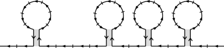
Figure 12. Folding off short loops. A loop can be folded off only when all of the three properties are satisfied. This ensures the result is a collection of tagged loops of length exactly $7$.

Let $T$ be some big odd number. We perform this folding procedure on each successive subword $v_{i}$ of a $(T,\epsilon)$-pseudorandom $w$ of length $T$ and obtain a collection of new words $v_{i}^{\prime}$ with trivalent vertices separated by even length intervals, such that length of $v_{i}^{\prime}$ and that of $v_{i}$ agree mod 9. Since $T$ is odd, we distinguish between even $v_{i}^{\prime}$, for which the trivalent vertices are an even distance from the initial vertex, and odd $v_{i}^{\prime}$, for which the trivalent vertices are an odd distance from the initial vertex.

By pseudorandomness, the reservoir consists of an almost equidistributed collection of short loops; i.e. the distribution differs from the uniform distribution by a multiplicative error of $\epsilon$. Furthermore, the words $v_{i}^{\prime}$ themselves are uniformly distributed with multiplicative error $\epsilon$, for each fixed possible value of $|v_{i}^{\prime}|$, and the same is true if one conditions on the $v_{i}^{\prime}$ being even or odd (in the sense above). This is because the distribution of random letters $v_{2}$ not equal to $v_{1}^{-1}$ that follow a subword of the form $v_{1}Pup$ averaged over all possible $Pup$ is just the uniform distribution on letters not equal to $v_{1}^{-1}$.

5.4. Random pairing of $v_{i}^{\prime}$

The $v_{i}^{\prime}$ fall into finitely many families depending on their lengths and parity — i.e. whether they are even or odd in the sense of the previous subsection. Moreover, for each fixed length and parity, the distribution of words is uniform up to multiplicative error $\epsilon$. Thus, for every reduced word $\sigma$ of suitable length, the number of $v_{i}^{\prime}$ of any given parity equal to $\sigma$ and the number equal to $\sigma^{-1}$ is very nearly equal.

For each $v_{i}^{\prime}$ let $v_{i}^{\prime\prime}$ denote the subword of $v_{i}^{\prime}$ excluding the first and last letter. We call a pair $v_{i}^{\prime}$ and $v_{j}^{\prime}$ compatible if they satisfy the following conditions:

1. the label on $v_{i}^{\prime\prime}$ is $\sigma$, and the label on $v_{j}^{\prime\prime}$ is $\sigma^{-1}$, for some $\sigma$ reduced;

2. the first letter of $v_{i}^{\prime}$ is not inverse to the last letter of $v_{j}^{\prime}$, and conversely;

3. if $|\sigma|$ is even, the parities of $v_{i}^{\prime}$ and $v_{j}^{\prime}$ are opposite, and if $|\sigma|$ is odd, the parities agree.

Let $v_{i}^{\prime}$ and $v_{j}^{\prime}$ be compatible. Then we can glue $v_{i}^{\prime\prime}$ to $v_{j}^{\prime\prime}$, and by condition (3) the trivalent vertices on either side are not identified. Furthermore, because of condition (2) the new boundary words that result from the gluing are still reduced. See Figure 13.

2pt $a$ at 158.5 19 $b$ at 151 15.5 $b$ at 147 17 $B$ at 136 18 $a$ at 135 14.8 $a$ at 123 14.8 $B$ at 119.7 18 $b$ at 108.5 19 $b$ at 104.9 15 $A$ at 95 15.5 $B$ at 91.5 18 $b$ at 81 19 $b$ at 78.5 15.2 $a$ at 68 15.5 $B$ at 57 15.6 $B$ at 43 15.6 $a$ at 39.3 18 $A$ at 28.2 19 $b$ at 26.3 15.5 $a$ at 14 15.5 $b$ at 6 19

$b$ at 6 2 $A$ at 11 5 $A$ at 15 2 $a$ at 25.4 1 $B$ at 28 5 $b$ at 40 4.8 $a$ at 44 2 $A$ at 53.5 2 $b$ at 56 5 $A$ at 65.5 5 $A$ at 69 2 $a$ at 79 1 $B$ at 81 5 $a$ at 92 5 $B$ at 106 5 $A$ at 119 5 $b$ at 124 2 $B$ at 134 2 $A$ at 137 5.5 $B$ at 149 5 $a$ at 158 2

Figure 13. Random pairing of the $v_{i}^{\prime}$. The shorter region which is entirely glued is $v_{i}^{\prime\prime}$. Note that the initial and final letters of the paired words are not inverse, so the gluing is limited to exactly the $v_{i}^{\prime\prime}$.

By pseudorandomness, we can glue all but $\epsilon$ of the total length of the remainder (excluding the reservoir) in this way, and we are left with some collection $\Gamma$ of cyclic words, where $|\Gamma|\leq\epsilon n$, plus the reservoir.

5.5. Gluing up $\Gamma$

The next step of the construction is elementary. We use some relatively small mass of small loops from the reservoir to pair up with $\Gamma$, so at the end of this step we are left only with loops in the reservoir. Furthermore, since (for a suitable choice of $\epsilon$) the mass of $\Gamma$ is so small, even compared to the mass of short loops of any given type, if we can do this construction while using at most $|\Gamma|$ short loops, the content of the reservoir at the end will still be almost equidistributed, with multiplicative error some new (but arbitrarily small) constant $\epsilon^{\prime}$.

We claim that for any positive $m$ we can glue $m-6$ (or at most $3$ if $m<7$) short loops together to create a trivalent partial fatgraph with unglued part a loop of length $m$. The cases $m<7$ are elementary, and for $m=7$ one can take a single short loop with no gluing at all. We prove the general case by induction, by proving the stronger statement that the trivalent fatgraph of length $m\geq 7$ can be chosen to contain a pair of adjacent segments in its boundary of length $4$ and $3$ each containing no trivalent vertex in the interior. This is obviously true for $m=7$. Suppose it is true for $m$, and denote the adjacent segments by $\cdot 4\perp 3\cdot$. We can “bracket” this as $\cdot 3(1\perp 2)2\cdot$ and bracket another short loop as $4(1\perp 2)$. Gluing the two (bracketed) segments of length 3, we see obtain a loop of length $m+1$ containing $\cdot 3\perp 4\perp 2\cdot$, completing the induction step and proving the claim. See Figure 14.

2pt

Figure 14. Attaching a loop of length 7 as shown increases the total loop length by $1$. By induction, we create a trivalent partial fatgraph with one unglued loop of any size. We can then label the fatgraph arbitrarily such that the unglued loop is any desired word.

If we choose suitable short loop types, the labels on the resulting partial fatgraph and the edges incident to the trivalent vertices can be arbitrary, so we can build a loop that can be used to cancel a loop of $\Gamma$.

5.6. Linear programming

Finally, we are left with a reservoir of almost equidistributed short loops. Since our original collection of words had homologically trivial sum, the same is true for the reservoir. We will show that any homologically trivial collection of almost equidistributed short loops can be glued up entirely, thus completing the construction of the $f$-folded fatgraph $X$, and the proof of Theorem 4.16. In fact, it is easier to show that a multiple of any such collection can be glued up; thus the fatgraph we build will be assembled from the disjoint union of copies of the partial fatgraphs built so far, glued up along the collection of short loops, and $\partial^{\pm}$ will consist of the same number of disjoint copies of $[a,b]$ and $\phi([b,a])$. This is evidently enough to prove the theorem.

The advantage of allowing ourselves to use multiple copies is that we can find a solution to the gluing problem “over the rationals”. Formally, let $\mathcal{L}$ denote the vector space spanned by the set of types of short loops, let $\mathcal{L}^{+}$ denote the cone of vectors with non-negative coefficients, and let $\mathcal{L}^{+}_{0}$ denote the subcone of homologically trivial vectors. The “uniform” vector ${\bf 1}$ is the vector with all coefficients 1. This is in $\mathcal{L}^{+}_{0}$. Denote by $C$ the non-negative linear span of the vectors representing collections that can be glued up. Then any rational vector in $C$ can be “projectively” glued up. It is easy to see that ${\bf 1}$ is in $C$; we will show that $C$ contains an open neighborhood of the ray spanned by ${\bf 1}$. Since our collection of short loops is almost equidistributed, it will be contained in this open neighborhood, and we will be done. We call a vector feasible if it is in $C$.

Proposition 5.3.

In the above notation and in a rank $2$ free group, $C$ contains an open projective neighborhood of the ray spanned by ${\bf 1}$. That is, there is some $\epsilon>0$ such that $C$ contains an $\epsilon$ neighborhood of ${\bf 1}$ and thus contains all scalar multiples of this neighborhood.

Proposition 5.3 is actually proved with a computation. We defer the proof and show how the arbitrary rank case reduces to rank 2. First we give some notation necessary for the proof. We define a function $\iota$ on tagged loops which takes a loop $v$ to $v^{-1}$, with the tag in the diametrically opposite position. When the tag switches positions under $\iota$, there is a choice about what the tag becomes, because there is more than one possible tag at each location in a word. Choose tags arbitrarily such that $\iota$ is an involution. Notice that for any loop $\gamma$, there is an annulus (trivalent fatgraph) with boundary $\gamma+\iota(\gamma)$. We call this an $\iota$-annulus.

Proposition 5.4.

In the above notation and for any finite rank free group, $C$ contains an open projective neighborhood of the ray spanned by ${\bf 1}$.

Proof.

Suppose we are given any vector $v\in\mathcal{L}^{\prime+}_{0}$. We must show that there is some $n$ such that $v+n{\bf 1}$ bounds a trivalent fatgraph. This will prove the proposition. Therefore, we need to understand when a collection of loops, plus an arbitrary multiple of ${\bf 1}$, bounds a trivalent fatgraph.

Given a collection of tagged loops $S$ and a single loop $\gamma$, suppose we can exhibit a trivalent fatgraph $Y$ with boundary $\gamma+\sum_{i}\alpha_{i}$. We say that $\gamma$ is fatgraph equivalent to $\sum_{i}\iota(\alpha_{i})$. Now, if we can find a trivalent fatgraph with boundary $S+\sum_{i}\iota(\alpha_{i})$, then the union of this trivalent fatgraph with $Y$ has boundary $S+\sum_{i}\iota(\alpha_{i})+\alpha_{i}+\gamma$. In other words, we have a trivalent fatgraph with boundary $S+\gamma$, plus two $\iota$ pairs. If we then add all other remaining $\iota$ pairs, we can simply add $\iota$-annuli to get a trivalent fatgraph with boundary $S+\gamma+{\bf 1}$.

Therefore, for the purpose of finding a trivalent fatgraph with a given boundary $S$ modulo adding some multiple of ${\bf 1}$, if we have some loop $\gamma\in S$, and we find a collection of loops $\sum_{i}\alpha_{i}$ which is fatgraph equivalent to $\gamma$, then we can throw out $\gamma$ from $S$, replace it with $\sum_{i}\alpha_{i}$, and find a trivalent fatgraph bounding what remains. To reduce to rank $2$, we’ll show that any loop is fatgraph equivalent to a collection of loops, each of which contains only two generators. After showing this, we’ll explain how to apply Proposition 5.3 to complete the proof.

Lemma 5.5.

Every loop is fatgraph equivalent to a collection of loops, each containing at most two generators.

Proof.

To show that a loop is fatgraph equivalent to another collection of loops, note that it suffices to show it for untagged loops, provided there are positions on the fatgraph $Y$ to place tags. This is because a loop is fatgraph equivalent to itself with a different tag position, for $\gamma+\gamma^{\prime-1}$ bounds a trivalent tagged annulus, where $\gamma^{\prime-1}$ is $\iota(\gamma)$ with the tag in a different position.

Thus, suppose we are given a loop $\gamma$ containing more than $2$ generators. We partition $\gamma$ into runs of a single generator, and because $\gamma$ has at least $3$ generators, we can write, $\gamma=abcx$, where $a$, $b$, and $c$ are runs of distinct generators, and $x$ is the remainder of $\gamma$, which might be empty. Abusing notation, we will write $a$, $b$, $c$ to denote a run of any size of the $a$, $b$, $c$ generators. The trivalent fatgraph shown in Figure 15 has boundary of the form $abcx+Bc+bA+CaX$. Note that this fatgraph is trivalent; it cannot fold by the assumption that $a$, $b$, $c$ are maximal runs of distinct generators. Also, the edge lengths can be chosen so that all the loops have size $7$.

2pt $a$ at 34 74 $b$ at 55 34 $c$ at 26 11 $x$ at 10 48

$B$ at 70 34 $B$ at 81 60 $c$ at 82 22

$A$ at 43 88 $b$ at 81 76 $A$ at 72 97

$X$ at -5 50 $C$ at 15 -3 $C$ at 94 11 $a$ at 100 104

Figure 15. A trivalent fatgraph showing how a loop of the form $abcx$ is fatgraph equivalent to two loops containing only two generators, plus a loop of the form $XcA$.

Therefore, $abcx$ is fatgraph equivalent to two loops with two generators, plus one loop of the form $Acx$. The latter loop has, then, fewer runs, and we can repeat this procedure until $Acx$ contains only two generators. At that point, we have shown that $\gamma$ is fatgraph equivalent to a collection of loops, each of which contains at most two generators. ∎

Now we can complete the proof of Proposition 5.4. Given a vector $v\in\mathcal{L}^{\prime+}_{0}$, we may take a sufficient multiple to assume that $v$ is integral. Let $S$ be the collection of loops represented by $v$. We’ve shown that $S$ is fatgraph equivalent to a collection of loops $S^{\prime}$, where each loop in $S^{\prime}$ contains at most two generators. We can write $S^{\prime}=\bigcup_{\{x,y\}}S^{\prime}_{x,y}$, where each $S^{\prime}_{x,y}$ contains the loops in $S^{\prime}$ containing the generators $x$ and $y$. There is an ambiguity about where to put loops which contain a single generator; place them arbitrarily, though we will rearrange them presently. Now, each collection $S^{\prime}_{x,y}$ might not be homologically trivial. However, after multiplying the original vector $v$ by $7$, we may assume that the homological defect of each generator in each collection is a multiple of $7$. Therefore, we can make each collection $S^{\prime}_{x,y}$ homologically trivial by redistributing the loops consisting of a single generator (or, if necessary, introducing $\iota$ pairs).

Since each collection $S^{\prime}_{x,y}$ is homologically trivial, we can apply Proposition 5.3 to find a trivalent fatgraph with boundary $S^{\prime}_{x,y}+{\bf 1}_{x,y}$, where ${\bf 1}_{x,y}$ denotes the uniform vector in the set of loops containing generators $x$ and $y$. Taking the union of these fatgraphs over all $x$, $y$, yields a trivalent fatgraph which shows that $S^{\prime}=\bigcup_{\{x,y\}}S^{\prime}_{x,y}$ is fatgraph equivalent to a collection of $\iota$ pairs, and therefore fatgraph equivalent to the empty set. That is, the collection $S$ represented by our original vector $v$ is fatgraph equivalent to the empty set, which is to say that there is a trivalent fatgraph with boundary $S+n{\bf 1}$, for $n$ sufficiently large. This completes the proof. ∎

We now give the proof in the rank $2$ case, or rather, a description of the computation which proves it.

Proof of Proposition 5.3.

We wish to show that the cone $C$ contains an open projective neighborhood of ${\bf 1}$. To start, we describe some necessary background about cones and linear programming. Determining if a point lies in the interior of the cone on a set of vectors can be phrased as a linear programming problem by using the following lemma.

Lemma 5.6.

Let $x,v_{1},\ldots,v_{k}\in\mathbb{R}^{n}$. If the $v_{i}$ span $\mathbb{R}^{n}$ and there is an expression $x=\sum_{i}t_{i}v_{i}$ with $t_{i}>0$ for all $i$, then $x$ lies in the interior of the cone spanned by the $v_{i}$.

Proof.

To show that $x$ lies in the interior, it suffices to show that $x$ is not contained in any supporting hyperplane. Thus, let $H$ be any supporting hyperplane for the cone spanned by the $v_{i}$. Because the $v_{i}$ span $\mathbb{R}^{n}$, there is some $j$ so that $v_{j}$ is not in $H$. We have expressed $x=\sum_{i}t_{i}v_{i}$ with, in particular, $t_{j}>0$. Therefore, if we decompose $\mathbb{R}^{n}=H\oplus\textnormal{span}\{v_{j}\}$, and express $x$ in this decomposition, we will find that the coefficient of $v_{j}$ is not zero, so $x$ is not contained in $H$. ∎

Using Lemma 5.6, we observe that if we are given the $v_{i}$ as the columns of the matrix $M$, and $x$ is a column vector, then a feasible point $y$ for the problem $Ay=x$, $y\geq 1$ provides a certificate that $x$ is contained in the interior. Feasibility testing can be phrased as a linear programming problem by setting the objective function to zero. We remark that the lower bound on $y$ is arbitrary; if $x$ is in the interior, the linear program will succeed for some lower bound, but we don’t know a priori what it is.

The proof of Proposition 5.3 therefore reduces to the following computation.

1. Find a collection of vectors $V$ in the cone $C$ which together span the space $\mathcal{L}_{0}$.

2. Show that the uniform vector ${\bf 1}$ lies in the cone on $V$.

To find $V$, we simply tried many random vectors in $\mathcal{L}_{0}$ and checked if they were contained in $C$ by checking if they bounded a trivalent fatgraph. Both steps (1) and (2) require linear programming: in order to check that a vector bounds a trivalent fatgraph, we solve a linear programming problem derived from the scallop algorithm ([10]), and to show that the uniform vector lies in the cone on $V$, we solve the linear programming problem derived from Lemma 5.6.

In order to make the many linear programming problems in step (1) feasible, we need to choose low-density vectors; that is, vectors with a small number of nonzeros. Recall there are $4376$ short loops of length $7$ and rank $2$, and the space of homologically trivial linear combinations has dimension $4374$. We found a collection of $9626$ vectors, each with $8$ nonzeros, which span this $4374$-dimensional space. This required solving a few tens of thousands of small linear programming problems (i.e. runs of scallop), which was easily accomplished using the linear programming backend GLPK[13]. As we built this collection, we occasionally ran a much larger linear program to determine if the uniform vector was contained in the cone (not necessarily in the interior, as that is more difficult to solve in practice). Once our cone did contain the uniform vector, we ran one final linear program to verify that it lay in the interior.

Even though these latter linear programs had only a few thousand columns and a few thousand rows, they proved quite difficult in practice. Fortunately, the proprietary software package Gurobi[18], which offers a free academic license, was able to solve them in a few minutes. We used Sage[27] to facilitate many of the final steps. ∎

Remark 5.7.

It is important to highlight that the initial steps of the proof of the random $f$-folded surface theorem reduce the problem of finding a folded surface whose boundary is a given random loop to the problem of showing that a collection of tagged loops of a uniformly bounded size ($7$) bounds a folded fatgraph, provided this collection is sufficiently close to uniform. Proposition 5.4 shows that, indeed, a collection of tagged loops of size $7$ sufficiently close to uniform does bound a folded fatgraph. We emphasize that this linear programming is done once to solve this latter, uniformly bounded, one-time problem.

This completes the proof of Theorem 4.16.

5.7. Sapir’s group

Definition 5.8.

We define Sapir’s group $C$ to be the HNN extension of $F_{2}:=\langle a,b\rangle$ by the endomorphism $\phi:a\to ab,b\to ba$.

In [25], Problem. 8.1, Sapir posed explicitly the problem of determining whether $C$ contains a closed surface subgroup, and in fact conjectured (in private communication) that the answer should be negative. This group was also studied by Crisp–Sageev–Sapir and (independently) Feighn, who sought to find a surface subgroup or show that one did not exist. Because of the attention this particular question has attracted, we consider it significant that our techniques are sufficiently powerful to give a positive answer:

Theorem 5.9.

Sapir’s group $C$ contains a closed surface subgroup of genus 28.

Proof.

The theorem is proved by exhibiting an explicit $f$-folded surface. Figure 16 indicates a fatgraph whose fattening has four boundary components, three of which are (conjugates of) $babaBABA$ and the fourth of which is $\phi^{4}(babaBABA)^{-3}$. The blue circles mark the $babaBABA$ components. By taking a 3-fold cover we obtain a fatgraph whose fattening has six boundary components, three of which are conjugates of $(babaBABA)^{3}$, and three of which are conjugates of $\phi^{4}(babaBABA)^{-3}$. In the HNN extension $F*_{\phi}$ we can glue these boundary components in pairs, giving a closed surface $S$ together with a map $\pi_{1}(S)\to F*_{\phi}$.

The surface is $f$-folded, and therefore the resulting map of the surface group is injective. To see this, note that the $babaBABA$ components are disjoint from each other, the underlying fatgraph is Stallings folded, and the $f$-vertices (indicated in red) are all 2-valent.

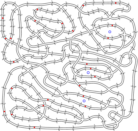
Figure 16. A fatgraph bounding $3\cdot babaBABA+\phi^{4}(babaBABA)^{-3}$

∎

Remark 5.10.

In fact, Sapir expressed the opinion that “most” ascending HNN extensions of free groups should not contain surface subgroups, which is contradicted by the Random $f$-folded Surface Theorem 4.16. On the other hand, the probabilistic estimates involved in the proof of this theorem are only relevant for endomorphisms taking generators to very long words, and therefore Sapir’s group seems to be an excellent test case.

References

- [1] C. Bavard, Longueur stable des commutateurs, Enseign. Math. (2), 37, 1-2, (1991), 109–150
- [2] M. Bestvina and M. Handel, Train tracks and automorphisms of free groups, Ann. Math. 135 (no. 1), (1992), 1–51
- [3] R. Brooks, Some remarks on bounded cohomology, Riemann surfaces and related topics: Proceedings of the 1978 Stony Brook Conference (State Univ. New York, Stony Brook, N.Y., 1978), pp. 53–63, Ann. of Math. Stud., 97, Princeton Univ. Press, Princeton, N.J., 1981
- [4] D. Calegari, Surface subgroups from homology, Geom. Topol. 12 (2008), no. 4, 1995–2007
- [5] D. Calegari, scl, MSJ Memoirs, 20. Mathematical Society of Japan, Tokyo, 2009.
- [6] D. Calegari, Stable commutator length is rational in free groups, Jour. Amer. Math. Soc. 22 (2009), no. 4, 941–961
- [7] D. Calegari and A. Walker, Random rigidity in the free group, Geom. Topol. 17 (2013), 1707–1744
- [8] D. Calegari and A. Walker, Isometric endomorphisms of free groups, New York Journal of Math, 17 (2011) 713–743
- [9] D. Calegari and A. Walker, Surface subgroups from linear programming, version 1, preprint, arXiv:1212.2618v1
- [10] D. Calegari and A. Walker, scallop, computer program available from the authors’ webpages, and from computop.org
- [11] J. Crisp, M. Sageev and M. Sapir, Surface subgroups of right-angled Artin groups, Internat. J. Algebra Comput. 18 (2008), no. 3, 443–491
- [12] M. Culler, Using surfaces to solve equations in free groups, Topology 20 (1981), no. 2, 133–145
-
[13]
GNU Linear Programming Kit, Version 4.45,
http://www.gnu.org/software/glpk/glpk.html - [14] C. Gordon, D. Long and A. Reid, Surface subgroups of Coxeter and Artin groups, J. Pure Appl. Algebra 189 (2004), no. 1–3, 135–148
- [15] C. Gordon and H. Wilton, On surface subgroups of doubles of free groups, J. Lond. Math. Soc. (2) 82 (2010), no. 1, 17–31
- [16] R. Grigorchuk, Some results on bounded cohomology, Combinatorial and geometric group theory (Edinburgh, 1993), 111–163 LMS Lecture Note Ser. 204, Cambridge Univ. Press, Cambridge, 1995
- [17] M. Gromov, Volume and bounded cohomology, Inst. Hautes Études Sci. Publ. Math. (1982), no. 56, 5–99
-
[18]
Gurobi Optimization, Inc.,
Gurobi Optimizer Reference Manual (2012),
http://www.gurobi.com - [19] J. Kahn and V. Markovic, Immersing almost geodesic surfaces in a closed hyperbolic three manifold, Ann. of Math. (2) 175 (2012), no. 3, 1127–1190
- [20] S.-H. Kim and S.-I. Oum, Hyperbolic surface subgroups of one-ended doubles of free groups, J. Topology, to appear
- [21] S.-H. Kim and H. Wilton, Polygonal words in free groups, Q. J. Math. 63 (2012), no. 2, 399–421
- [22] R. Penner, Perturbative series and the moduli space of Riemann surfaces, J. Diff. Geom. 27 (1988), 35–53
- [23] P. Reynolds, Dynamics of Irreducible Endomorphisms of , preprint; arXiv:1008.3659
- [24] A. Rhemtulla, A problem of bounded expressibility in free products, Proc. Cambridge Philos. Soc. 64 (1968), 573–584
- [25] M. Sapir, Some group theory problems, Internat. J. Algebra Comput. 17 (2007), no. 5–6, 1189–1214
- [26] J. Stallings, Topology of finite graphs, Invent. Math. 71 (1983), no. 3, 551–565
- [27] W. A. Stein et al., Sage Mathematics Software (Version 5.3), The Sage Development Team (2012) http://www.sagemath.org.
- [28] W. Thurston, A norm for the homology of 3-manifolds, Mem. AMS 59 (1986), no. 339, i–vi and 99–130
- [29] A. Walker, gallop, computer program available from the author’s webpage
- [30] A. Walker, wallop, computer program available from the author’s webpage