The first-crossing area of a diffusion process with jumps over a constant barrier

Abstract

For a given barrier $S$ and a one-dimensional jump-diffusion process $X(t),$ starting from $x<S,$ we study the probability distribution of the integral $A_{S}(x)=\int_{0}^{\tau_{S}(x)}X(t)\ dt$ determined by $X(t)$ till its first-crossing time $\tau_{S}(x)$ over $S.$ In particular, we show that the Laplace transform and the moments of $A_{S}(x)$ are solutions to certain partial differential-difference equations with outer conditions. The distribution of the minimum of $X(t)$ in $[0,\tau_{S}(x)]$ is also studied. Thus, we extend the results of a previous paper by the author, concerning the area swept out by $X(t)$ till its first-passage below zero. Some explicit examples are reported, regarding diffusions with and without jumps.

Keywords: First-crossing time, first-crossing area, one-dimensional jump-diffusion.
Mathematics Subject Classification: 60J60, 60H05, 60H10.

1 Introduction

This paper deals with the first-crossing area, $A_{S}(x)=\int_{0}^{\tau_{S}(x)}X(t)\ dt,$ determined by a one-dimensional jump-diffusion process $X(t)$ starting from $x,$ till its first-crossing time, $\tau_{S}(x),$ over a threshold $S>x,$ and it extends the results of a previous paper by the author ([2]), concerning the area swept out by $X(t)$ till its first-passage below zero. As for results about the integral of $X(t)$ over a deterministic and fixed time interval, see e.g [5].

Notice that $A_{S}(x)=\overline{X}_{[0,\tau_{S}(x)]}\cdot\tau_{S}(x),$ where $\overline{X}_{[0,\tau_{S}(x)]}$ denotes the time average of $X(t)$ over the interval $[0,\tau_{S}(x)].$

The first-crossing area has interesting applications in Biology, for instance in the framework of diffusion models for neural activity, if one identifies $X(t)$ with the neuron voltage at time $t,$ and $\tau_{S}$ with the instant at which the neuron fires, i.e. $X(t)$ exceeds the potential threshold value $S;$ then, $A_{S}/\tau_{S}$ represents the time average of the neural voltage till the first-crossing time over $S.$ Another application can be found in Queueing Theory, if $X(t)$ represents the length of a queue at time $t,$ and one identifies the first-passage time $\tau_{S}$ over the threshold $S$ with the overflow time, that is the instant at which the queue system first collapses; then, the first-crossing area represents the cumulative waiting time experienced by all the “users” till the congestion time.

As for an example from Economics, let us suppose that the variable $t$ represents the quantity of a commodity that producers have available for sale and $Y(t)$ describes the price of the commodity as a function of the quantity in a supply-and-demand model. Let us assume that $Y(t)$ is bounded between $0$ and $S>0,$ and consider the distance of $Y(t)$ from $S,$ that is the process $X(t):=S-Y(t).$ If we denote by $\tau$ the amount of product at which $Y(t)$ falls to zero (i.e. $X(t)$ reaches the value $S),$ then $\int_{0}^{\tau}X(t)dt=\tau S-\widetilde{A},$ where $\widetilde{A}=\int_{0}^{\tau}Y(s)ds$ provides a measure of the total value that consumers receive from consuming the amount $\tau$ of the product.

In the present article, we complete the study carried out in [2]; in fact, for a one-dimensional jump-diffusion process, in place of the first-passage area below zero, we consider the analogous problem of first-crossing area over a positive barrier.

Precisely, let be given a barrier $S>0$ and a one-dimensional jump-diffusion process $X(t),$ starting from $x<S;$ our aim is to study the probability distribution of the integral

$A_{S}(x)=\int_{0}^{\tau_{S}(x)}X(t)\ dt$ determined by $X(t)$ till its first-crossing time $\tau_{S}(x)$ over $S.$ We improperly call $A_{S}(x)$ “the first-crossing area of $X(t)$ over $S$”. Indeed, the area of the plane region determined by the trajectory of $X(t)$ and the $t$-axis in the first-crossing period $[0,\tau_{S}(x)]$ is $\int_{0}^{\tau_{S}(x)}|X(t)|\ dt$ which coincides with $A_{S}(x)$ only if $X(t)$ is non-negative in the entire interval $[0,\tau(x)].$

Since the topic was studied quite extensively in [2] (though in the slight different situation of first passage below zero), we will omit some details. We will suppose that $X(t)$ is the solution of a stochastic differential equation of the form:

$$dX(t)=b(X(t))dt+\sigma(X(t))dB_{t}+\int_{-\infty}^{+\infty}\gamma(X(t),u)\nu(dt,du)$$ (1.1)

with assigned initial condition $X(0)=x;$ here $B_{t}$ is a standard Brownian motion, $\nu(\cdot,\cdot)$ is a temporally homogeneous Poisson random measure (see Section 2 for the definitions), and the functions $b(\cdot),\sigma(\cdot),\gamma(\cdot,\cdot)$ satisfy suitable conditions for the existence and uniqueness of the solution (see Section 2). The coefficients regulate the drift $(b),$ the diffusion $(\sigma),$ and the sizes of the jumps $(\gamma)$ which occur at (random) exponentially distributed time intervals.

The process $X(t)$ which is the solution of the equation (1.1) reduces to a simple diffusion (i.e. without jumps) if $\gamma(x,u)=0,$ and in particular to Brownian motion with drift $\mu$ if $b(x)=\mu$ and $\sigma(x)=1.$

Denote by

$$\tau_{S}(x)=\inf\{t>0:X(t)\geq S|X(0)=x\}$$

the first-crossing time over $S$ of the process $X(t)$ starting from $x<S,$ and assume that $\tau_{S}(x)$ is finite with probability one. We will study the probability distributions of $\tau_{S}(x)$ and of the integral $A_{S}(x)=\int_{0}^{\tau_{S}(x)}X(t)\ dt,$ as well as their moments; moreover, the distribution of the minimum of $X(t)$ in $[0,\tau_{S}(x)]$ will be studied. In particular, we will show that the Laplace transforms of $A_{S}(x)$ and $\tau_{S}(x),$ their moments, as well as the probability distribution of the minimum of $X(t),$ are solutions to certain partial differential-difference equations (PDDEs) with outer conditions.

The paper is organized in the following way: Section 2 contains the statement of the problem and main results, in Section 3 some explicit examples are reported. Finally, Section 4 is devoted to conclusions and final remarks.

2 Notations, formulation of the problem and main results

Let $X(t)\in I:=(\alpha,\beta),\ -\infty\leq\alpha<\beta\leq+\infty,$ a time-homogeneous, one-dimensional jump-diffusion process which satisfies the stochastic differential equation (SDE) (1.1) with assigned initial condition $X(0)=x,$ where $B_{t}$ is a standard Brownian motion and $\nu(\cdot,\cdot)$ is a Poisson random measure on $(0,\infty)\times\rm I\!R.$ Then, $X(t)$ can be represented as

$$X(t)=x+\int_{0}^{t}b(X(s))ds+\int_{0}^{t}\sigma(X(s))dB_{s}+\int_{0}^{t}\int_{-\infty}^{+\infty}\gamma(X(s),u)\nu(ds,du)$$ (2.1)

For the definitions of the integrals in the right hand side of (2.1) and the Poisson measure, see [12]. The coefficients $b,\sigma$ and $\gamma$ completely specify the law of $X(t).$ In particular, an atom $(t,u)$ of the Poisson random measure $\nu$ causes a jump from $x$ to $x+\gamma(x,u)$ at time $t,$ if $X(t^{-})=x.$ We assume that $\nu$ is homogeneous with respect to time translation, that is, its intensity measure $E(\nu(dt,du))$ is of the form

$$E[\nu(dt,du)]=dt\pi(du)$$ (2.2)

for some positive measure $\pi$ defined on ${\cal B}(\rm I\!R)$  $({\cal B}(\rm I\!R)$ denotes the Borel $\sigma-$field of subsets of $\rm I\!R),$ and we suppose that the jump intensity

$$\Theta=\int_{-\infty}^{+\infty}\pi(du)\geq 0$$ (2.3)

is finite.

We make the following assumptions on the coefficients:

A1 $b,\sigma:I\rightarrow\rm I\!R$ are continuous functions and a constant $K>0$ exists, such that, for every $x,y\in I:$

$$|b(x)-b(y)|\leq K|x-y|$$

$$b^{2}(x)+\sigma^{2}(x)\leq K(1+x^{2})$$

A2 $\sigma$ is a non-negative, bounded function and it is differentiable for every $x$ belonging to the interior of $I.$ Moreover, there exists a strictly increasing function $G:\rm I\!R^{+}\rightarrow\rm I\!R$ such that $G(0)=0,\ \int_{0^{+}}G^{-2}(s)ds=+\infty$ and

$$|\sigma(x)-\sigma(y)|\leq G(|x-y|)$$

for every $x,y\in I.$

B1 For every $u$ and $x\in I:$

$$\int_{-\infty}^{+\infty}\gamma^{2}(x,u)\pi(du)\leq K(1+x^{2})$$

B2 For every $u$ and $x,y\in I:$

$$\int_{-\infty}^{+\infty}|\gamma(x,u)-\gamma(y,u)|\pi(du)\leq K|x-y|$$

Remark 2.1

The conditions A1, A2, and B1, B2 ensure that there exists a unique non-explosive solution of (1.1) which is a temporally homogeneous Markov process (see [12], [15]); A2 holds, for instance, if $\sigma(\cdot)$ is Lipschitz-continuous ($G(x)=const\cdot x)$, or H${\rm\ddot{o}}$lder-continuous of order $\alpha\in[1/2,1)$  ($G(x)=const\cdot x^{\alpha}).$

Notice that, if $\gamma=0,$ or $\nu=0,$ then the SDE (1.1) becomes the usual It${\rm\hat{o}}$’s stochastic differential equation for a simple-diffusion (i.e. without jumps).

In the special case when the measure $\pi$ is concentrated over the set $\{u_{1},u_{2}\}=\{-1,1\}$ with $\pi(u_{i})=\theta_{i}$ and $\gamma(u_{i})=\epsilon_{i},$ we can rewrite the SDE (1.1) as

$$dX(t)=b(X(t))dt+\sigma(X(t))dB_{t}+\epsilon_{2}dN_{2}(t)+\epsilon_{1}dN_{1}(t)$$ (2.4)

where $\epsilon_{1}<0,\ \epsilon_{2}>0$ and $N_{i}(t),t\geq 0$ are independent homogeneous Poisson processes of amplitude $1$ and rates $\theta_{1}$ and $\theta_{2},$ respectively governing downward $(N_{1})$ and upward $(N_{2})$ jumps.

Let $D$ be the class of function $f(t,x)$ defined in $\rm I\!R^{+}\times I,$ differentiable with respect to $t$ and twice differentiable with respect to $x,$ for which the function $f(t,x+\gamma(x,u))-f(t,x)$ is $\pi-$integrable for any $(t,x).$ We recall the generalized It${\rm\hat{o}}$’s formula for jump-diffusion processes giving the differential of a function $f\in D$ (see [12]):

$$df(t,X(t))=\left[\frac{\partial f}{\partial t}(t,X(t))+b(X(t))\frac{\partial f}{\partial x}(t,X(t))+\frac{1}{2}\sigma^{2}(X(t))\frac{\partial^{2}f}{\partial x^{2}}(t,X(t))\right]dt$$ (2.5)

$$+\frac{\partial f}{\partial x}(t,X(t))\sigma(X(t))dB_{t}+\int_{-\infty}^{+\infty}[f(t,X(t)+\gamma(X(t),u))-f(t,X(t))]\nu(dt,du).$$

The differential operator associated to the process $X(t)$ which is the solution of (1.1), is defined for any function $f\in D$ by:

$$Lf(t,x)=L_{d}f(t,x)+L_{j}f(t,x)$$ (2.6)

where the “diffusion part” is

$$L_{d}f(t,x)=\frac{1}{2}\sigma^{2}(x)\frac{\partial^{2}f}{\partial x^{2}}(t,x)+b(x)\frac{\partial f}{\partial x}(t,x)$$

and the “jump part” is

$$L_{j}f(t,x)=\int_{-\infty}^{+\infty}[f(t,x+\gamma(x,u))-f(t,x)]\pi(du).$$

Then, from (2.5), taking expectation, one obtains

$$E[f(t,X(t))]=f(0,X(0))+E\left(\int_{0}^{t}\left[\frac{\partial f}{\partial s}(s,X(s))+Lf(s,X(s))\right]ds\right).$$ (2.7)

For a barrier $S$ and $x<S,$ we define:

$$\tau_{S}(x)=\inf\{t>0:X(t)\geq S|X(0)=x\}$$ (2.8)

that is the first-crossing time over $S$ of $X^{x}(t)$ (i.e. the process $X(t)$ starting from $x)$ and suppose that $\tau_{S}(x)$ is finite with probability one. Really, it is possible to show (see [25], [8]) that the probability $p_{0}(x)$ that $X^{x}(t)$ ever leaves the interval $(-\infty,S)$ satisfies the partial differential-difference equation (PDDE):

$$Lp_{0}=0$$ (2.9)

with outer condition:

$$p_{0}(x)=1\ {\rm if}\ x\geq S.$$

The equality $p_{0}(x)=1$ is equivalent to say that $\tau_{S}(x)$ is finite with probability one. For diffusion processes without jumps (i.e. $\gamma=0)$ sufficient conditions are also available which ensure that $\tau_{S}(x)$ is finite w.p. 1, and they concern the convergence of certain integral associated to the coefficients of (1.1) (see Section 3.1 and also [12] , [14]).

Remark 2.2

Let us consider the special case when $X(t)=\widetilde{X}(t)+J(t),$ where $\widetilde{X}$ is a simple-diffusion (i.e. without jumps) and $J$ is a pure-jump process, set $\widetilde{m}(t)=E(\widetilde{X}(t)),$ and suppose that

$$\exists\ \bar{t}>0:\widetilde{m}(t)+E(J(t))>S,\ {\rm for\ any}\ t\geq\bar{t};$$ (2.10)

then, $P(\tau_{S}(x)<\infty)=1.$ Indeed, $P(\tau_{S}(x)=\infty)>0$ implies that, for a set of trajectories having positive probability, it results $X(t)<S$ for any $t\geq 0.$ Thus, by taking expectation one obtains $E(X(t))=\widetilde{m}(t)+E(J(t))<S$ for any $t\geq 0,$ which contradicts (2.10).

If $J(t)=\epsilon_{1}N_{1}(t)+\epsilon_{2}N_{2}(t)$ (cf. (2.4)), condition (2.10) becomes $\widetilde{m}(t)+(\epsilon_{1}\theta_{1}+\epsilon_{2}\theta_{2})t>S;$ in particular, for $\epsilon_{2}=\epsilon=-\epsilon_{1}$ it writes $\widetilde{m}(t)>S+\epsilon(\theta_{1}-\theta_{2})t.$

Let $U$ be a functional of the process $X;$ assume that $\tau_{S}(x)$ is finite with probability one, and for $\lambda>0$ denote by

$$M_{U,\lambda}(x)=E\left[e^{-\lambda\int_{0}^{\tau_{S}(x)}U(X(s))ds}\right]$$ (2.11)

the Laplace transform of the integral $\int_{0}^{\tau_{S}(x)}U(X(s))ds.$ Then, the following theorem holds (we omit the proof, since it is quite analogous to that of Theorem 2.3 in [2]):

Theorem 2.3

Let $X(t)$ be the solution of the SDE (1.1), starting from $X(0)=x<S;$ then, under the above assumptions, $M_{U,\lambda}(x)$ is the solution of the problem with outer conditions:

$$\begin{cases}LM_{U,\lambda}(x)=\lambda U(x)M_{U,\lambda}(x),\ x<S\\ M_{U,\lambda}(y)=1,\ {\rm for}\ y\geq S\\ \lim_{x\rightarrow-\infty}M_{U,\lambda}(x)=0\end{cases}$$ (2.12)

where $L$ is the generator of $X,$ which is defined by (2.6).

$\Box$

We recall that the n-th order moment of $\int_{0}^{\tau_{S}(x)}U(X(s))ds,$ if it exists finite, is given by $(n=1,2,\dots):$

$$T_{n}(x)=E\left[\left(\int_{0}^{\tau_{S}(x)}U(X(s))ds\right)^{n}\right]=(-1)^{n}\left[\frac{\partial^{n}}{\partial\lambda^{n}}M_{U,\lambda}(x)\right]_{\lambda=0}.$$

Then, taking the n-th derivative with respect to $\lambda$ in both members of the equation (2.12), and calculating it for $\lambda=0,$ one easily obtains that the n-th order moment $T_{n}(x)\ (n=1,2,\dots)$ of $\int_{0}^{\tau_{S}(x)}U(X(s))ds,$ whenever it exists finite, is the solution of the PDDE:

$$LT_{n}(x)=-nU(x)T_{n-1}(x),\ \ x<S$$ (2.13)

which satisfies

$$T_{n}(x)=0,\ {\rm for}\ x\geq S$$ (2.14)

and an appropriate additional condition.

Indeed, the only condition $T_{n}(x)=0$ for $x\geq S$ is not sufficient to determinate uniquely the desired solution of the PDDE (2.13), because it is a second order equation. We will return to this problem when we will consider some explicit examples. Note that for a diffusion without jumps $(\gamma=0)$ and for $U(x)\equiv 1,$ (2.13) is nothing but the celebrated Darling and Siegert’s equation ([11]) for the moments of the first-passage time, and (2.14) becomes simply the boundary condition $T_{n}(S)=0.$

Remark 2.4

In certain cases, the first-crossing time and the first-crossing area of $X(t)$ over $S$ can be expressed in terms of the first-passage time and the first-passage area of a suitable process below zero. For instance, let $X(t)=x+B_{t}+\mu t,$ with $\mu>0,$ i.e. Brownian motion with positive drift $\mu;$ then $\tau_{S}(x)=\inf\{t>0:X(t)\geq S\}$ has the same distribution as $\inf\{t>0:S-x+B_{t}-\mu t\leq 0\}\equiv\widetilde{\tau}(S-x),$ where $\widetilde{\tau}(y)$ denotes the first-passage time of the process $Y(t)=y+B_{t}-\mu t$ below zero. Moreover, it is easy to see that

$$A_{S}(x)=\int_{0}^{\tau_{S}(x)}X(t)dt=S\cdot\widetilde{\tau}(S-x)-\widetilde{A}(S-x)$$ (2.15)

where $\widetilde{A}(y)$ denotes the area swept out by $Y(t)$ till its first-passage below zero.

Thus, the moments of $\tau_{S}(x)$ can be soon obtained by those of $\widetilde{\tau}(S-x),$ while by using (2.15), the mean of $A_{S}(x)$ can be obtained in terms of $E(\widetilde{\tau}(S-x))$ and $E(\widetilde{A}(S-x))$ (the first two moments of $\widetilde{\tau}$ and $\widetilde{A}$ were obtained in [2] ). Notice that, the computation of $E(A_{S}(x)^{2})$ requires instead also the knowledge of the covariance of $\widetilde{\tau}$ and $\widetilde{A}.$

Distribution of the minimum of $X(t).$

Now, we will study the probability distribution of the maximum downward displacement (i.e. the minimum) of the jump-diffusion $X(t)$ starting from $x<S,$ till its first passage over $S,$ that is, $\mathfrak{m}(x)=\min_{t\in[0,\tau_{S}(x)]}\{X(t)|X(0)=x\}.$ For any $z\leq x\leq S$ the event $\{\mathfrak{m}(x)>z\}$ is nothing but the event “$X(t)$ first exit the interval $[z,S]$ through the right end $S$”; so, by the well-known result about the exit probability of a jump-diffusion from the right end of an interval (see [8]), we obtain that $v(x):=P(\mathfrak{m}(x)>z),$ as a function of $x,$ is solution of the equation $Lv=0$ with conditions $v(y)=1,\ y\geq S;\ v(y)=0,\ y\leq z.$ Thus, we get:

Proposition 2.5

$P(\mathfrak{m}(x)\leq z)$ is the solution of the problem with outer conditions:

$$\begin{cases}Lw(x)=0,\ x\in(z,S)\\ w(y)=0,\ y\geq S\\ w(y)=1,\ y\leq z\end{cases}$$ (2.16)

$\Box$

3 A few examples

In this section we will compute explicitly the moments of $\tau_{S}(x)$ and those of the first-crossing area $A_{S}(x)$ for certain jump-diffusion processes. We start with considering diffusions without jumps.

3.1 Simple diffusions (i.e with no jump)

Let $X(t)$ be the solution of (1.1), with $\gamma\equiv 0,$ that is:

$$\begin{cases}dX(t)=b(X(t))dt+\sigma(X(t))dB_{t}\\ X(0)=x\end{cases}$$ (3.1)

In this case $\tau_{S}(x)\equiv\inf\{t>0:X(t)=S|X(0)=x\},$ that is the first-passage time of $X^{x}(t)$ through $S.$

Let us consider the functions ($c$ is a constant) :

$$\phi(x)=\exp\left(-\int_{c}^{x}\frac{2b(s)}{\sigma^{2}(s)}ds\right)$$ (3.2)

$$\xi(x)=\phi(x)\int_{c}^{x}\frac{2}{\sigma^{2}(s)\phi(s)}ds.$$ (3.3)

As it is well-known (see e.g [12]), a sufficient condition in order that $\tau_{S}(x)$ is finite with probability one, namely the boundary $S$ is attainable, is that the function $\xi(x)$ is integrable in a neighbor of $S.$

Since the generator $L$ coincides with its diffusion part $L_{d},$ by Theorem 2.3 we obtain that, for $x<S,$ $M_{U,\lambda}(x)=E\left[e^{-\lambda\int_{0}^{\tau_{S}(x)}U(X(s))ds}\right]$ is the solution of the problem with boundary conditions ($M^{\prime}$ and $M^{\prime\prime}$ denote first and second derivative with respect to $x)$ :

$$\begin{cases}\frac{1}{2}\sigma^{2}(x)M^{\prime\prime}_{U,\lambda}(x)+b(x)M^{\prime}_{U,\lambda}(x)=\lambda U(x)M_{U,\lambda}(x)\\ M_{U,\lambda}(S)=1\\ \lim_{x\rightarrow-\infty}M_{U,\lambda}(x)=0\end{cases}.$$ (3.4)

Moreover, by (2.13), (2.14) the n-th order moments $T_{n}(x)$ of $\int_{0}^{\tau(x)}U(X(s))ds,$ if they exist, satisfy the recursive ODEs:

$$\frac{1}{2}\sigma^{2}(x)T^{\prime\prime}_{n}(x)+b(x)T^{\prime}_{n}(x)=-nU(x)T_{n-1}(x),\ {\rm for}\ x<S$$ (3.5)

with the condition $T_{n}(S)=0,$ plus an appropriate additional condition.

Finally, as regards the minimum $\mathfrak{m}(x),$ it turns out that its distribution $F(z)=P(\mathfrak{m}(x)\leq z)$ is the solution of the problem with boundary conditions:

$$\begin{cases}Lw(x)=0,\ x\in(z,S)\\ w(z)=1\\ w(S)=0\end{cases}.$$ (3.6)

Example 1 (Brownian motion with drift $\mu>0)$

Let be $X(t)=x+\mu t+\sigma B_{t},$ with $\mu,\sigma>0$ and $0<x<S.$ Without loss of generality, we can assume $\sigma=1$ (otherwise, dividing by $\sigma$ one reduces to this case). Note that, since the drift is positive, $\tau_{S}(x)=\tau_{S}^{\mu}(x)=\inf\{t>0|X(t)=S\}$ is finite with probability one, for any $x<S.$ Taking $b(x)=\mu,\ \sigma(x)=1,$ the equation in (3.4) for $M_{U,\lambda}(x)=E(e^{-\lambda\int_{0}^{\tau_{S}^{\mu}(x)}U(X(s)ds})$ becomes

$$\frac{1}{2}M^{\prime\prime}_{U,\lambda}(x)+\mu M^{\prime}_{U,\lambda}(x)-\lambda U(x)M_{U,\lambda}(x)=0.$$ (3.7)

(i) The moment generating function of $\tau_{S}^{\mu}(x)$

By solving (3.7) with $U(x)=1,$ we explicitly obtain:

$$M_{U,\lambda}(x)=c_{1}e^{\rho_{1}x}+c_{2}e^{\rho_{2}x}$$

where $\rho_{1}=-\mu-\sqrt{\mu^{2}+2\lambda}<0,\ \rho_{2}=-\mu+\sqrt{\mu^{2}+2\lambda}>0;$ the constants $c_{1}$ and $c_{2}$ must be determined by the boundary conditions. Indeed, $M_{U,\lambda}(-\infty)=0$ gives $c_{1}=0,$ while $M_{U,\lambda}(S)=1$ implies $c_{2}=e^{(\mu-\sqrt{\mu^{2}+2\lambda})S}.$ Thus, we get:

$$M_{U,\lambda}(x)=E(\exp(-\lambda\tau_{S}^{\mu}(x))=\exp[(\mu-\sqrt{\mu^{2}+2\lambda})(S-x)].$$ (3.8)

This Laplace transform can be explicitly inverted (see [17]), so obtaining the well-known expression of the density of $\tau_{S}^{\mu}(x):$

$$f_{\tau_{S}^{\mu}(x)}(t)=\frac{S-x}{\sqrt{2\pi}t^{3/2}}e^{-(S-x-\mu t)^{2}/2t}.$$ (3.9)

For $\mu>0$ the moments $T_{n}(x)=E(\tau_{S}^{\mu}(x))^{n}$ of any order $n,$ are finite and they can be easily obtained by calculating $(-1)^{n}[\partial^{n}M_{U,\lambda}(x)/\partial\lambda^{n}]_{\lambda=0}.$ We obtain, for instance:

$$E(\tau_{S}^{\mu}(x))=\frac{S-x}{\mu},\ \ E((\tau_{S}^{\mu}(x))^{2})=\frac{S-x}{\mu^{3}}+\frac{(S-x)^{2}}{\mu^{2}}$$ (3.10)

(cf. Remark 2.4 and the results for BM with negative drift in [2] ). Note that $E(\tau_{S}^{\mu}(x))\rightarrow+\infty,$ as $\mu\rightarrow 0.$ As easily seen, for any $x<S$ it results $M_{U,\lambda}(x)\rightarrow 1,$ as $\mu\rightarrow+\infty,$ or, equivalently, $\tau_{S}^{\mu}(x)$ converges to $0$ in distribution, and so $E((\tau_{S}^{\mu}(x))^{n})\rightarrow 0,$ as $\mu\rightarrow+\infty,$ for any $n$ and $x<S.$

(ii) The moments of $A_{S}^{\mu}(x)=\int_{0}^{\tau_{S}^{\mu}(x)}(x+\mu t+B_{t})dt$

For $U(x)=x$ the equation (3.7) becomes

$$\frac{1}{2}M^{\prime\prime}_{U,\lambda}+\mu M^{\prime}_{U,\lambda}=\lambda xM_{U,\lambda}$$ (3.11)

with conditions $M_{U,\lambda}(S)=1,\ M_{U,\lambda}(-\infty)=0;$ now $M_{U,\lambda}(x)=E(e^{-\lambda A_{S}^{\mu}(x)}).$ Unfortunately, its explicit solution cannot be found in terms of elementary functions, but it can be written in terms of the Airy function (see [18], [13]) though it is impossible to invert the Laplace transform $M_{U,\lambda}$ to obtain the probability density of $A_{S}^{\mu}(x).$

In the special case $\mu=0,$ it can be shown (see [18], [2]) that the solution of (3.11) is:

$$M_{U,\lambda}(x)=3^{2/3}\Gamma\left(\frac{2}{3}\right){\rm Ai}(2^{1/3}\lambda^{1/3}(S-x))$$ (3.12)

where ${\rm Ai}(z)=\pi^{-1}\sqrt{z/3}\ K_{1/3}\left(\frac{2}{3}z^{3/2}\right)$ denotes the Airy function, and $K_{\nu}(z)$ is a modified Bessel function (see [1]). Calculating the derivative with respect to $\lambda$ in (3.12), we obtain:

$$\frac{\partial}{\partial\lambda}M_{U,\lambda}(x)=\left(\frac{2}{3}\right)^{1/3}\Gamma\left(\frac{2}{3}\right)(S-x){\rm Ai}^{\prime}(2^{1/3}\lambda^{1/3}(S-x))\cdot\lambda^{-2/3}$$

By using the fact that ${\rm Ai}^{\prime}(0)=-\left(3^{1/3}\Gamma\left(\frac{1}{3}\right)\right)^{-1}$ (see [1]), it follows that $\frac{\partial}{\partial\lambda}M_{U,\lambda}(x)|_{\lambda=0}=-\infty,$ namely, the expectation of $A_{S}^{0}(x)$ is infinite. Notice that, unlike the Laplace transform inversion reported in [2] for a similar case (see equation (3.12) therein), we are not able to invert explicitly the Laplace transform (3.12) to find the density of $A_{S}^{0};$ in fact, in the case considered in [2] this was possible, thanks to an integral identity (see e.g. [18], [13] ) involving the modified Bessel function, which serves the purpose when the support of the candidate density of $A_{S}^{0}$ is $(0,+\infty).$

For $\mu>0,$ we will find closed form expression for the first two moments of $A_{S}^{\mu}(x),$ by solving (3.5) with $U(x)=x.$ For $n=1,$ we get that $T_{1}(x)=E(A_{S}^{\mu}(x))$ must satisfy the equation:

$$\begin{cases}\frac{1}{2}T_{1}^{\prime\prime}(x)+\mu T_{1}^{\prime}(x)=-x\\ T_{1}(S)=0\end{cases}$$ (3.13)

Of course, the only condition $T_{1}(S)=0$ is not sufficient to uniquely determinate the solution. The general solution of (3.13) involves arbitrary constants $c_{1}$ and $c_{2}$ and, as easily seen, it is given by

$$T_{1}(x)=c_{1}+c_{2}e^{-2\mu x}-\frac{x^{2}}{2\mu}+\frac{x}{2\mu^{2}}\ .$$

By imposing that $T_{1}(S)=0$ and that for any $x\leq 0$ it must be $T_{1}(x)\rightarrow 0,$ as $\mu\rightarrow+\infty,$ we find that the mean first-crossing area is

$$E(A_{S}^{\mu}(x))=\frac{S-x}{2\mu}\left[S+x-\frac{1}{\mu}\right]$$ (3.14)

This formula also follows by taking expectation in (2.15), and using that $E(\widetilde{\tau}(y))=\frac{y}{\mu},$

$E(\widetilde{A}(y))=\frac{y^{2}}{2\mu}+\frac{y}{2\mu^{2}}$ (see [2]).

As far as the second moment of $A_{S}^{\mu}(x)$ is concerned, we have to solve (3.5) with $U(x)=x$ and $n=2,$ obtaining the equation for $T_{2}(x)=E[(A_{S}^{\mu}(x))^{2}]:$

$$\begin{cases}\frac{1}{2}T_{2}^{\prime\prime}(x)+\mu T_{2}^{\prime}(x)=-\frac{x}{\mu}(S-x)(S+x-1/\mu)\\ T_{2}(S)=0\end{cases}$$ (3.15)

As before, the only condition $T_{2}(S)=0$ is not sufficient to uniquely determinate the solution. The general solution of (3.15), which involves two arbitrary constants $c_{1}$ and $c_{2},$ is given by

$$T_{2}(x)=c_{1}+c_{2}e^{-2\mu x}+Ax^{4}+Bx^{3}+Cx^{2}+Dx,$$

where

$$A=\frac{1}{4\mu^{2}},\ B=-\frac{5}{6\mu^{3}},\ C=\frac{S}{4\mu^{4}}(2\mu+1-2\mu^{2}S),\ D=-\frac{S}{4\mu^{5}}(2\mu+1-2\mu^{2}S).$$

By imposing that, for any $x\leq 0$ it must be $T_{2}(x)\rightarrow 0,$ as $\mu\rightarrow+\infty,$ we find $c_{2}=0;$ moreover, by $T_{2}(S)=0$ we get $c_{1}=-(AS^{4}+BS^{3}+CS^{2}+DS).$ Thus the second order moment of the first-crossing area is

$$E[(A_{S}^{\mu}(x))^{2}]=A(x^{4}-S^{4})+B(x^{3}-S^{3})+C(x^{2}-S^{2})+D(x-S),$$ (3.16)

where the constants $A,B,C,D$ are as above. Finally, by (3.14) and (3.16), one can obtain the variance of $A_{S}^{\mu}(x).$

Notice that $E[(A_{S}^{\mu}(x))^{2}]$ has to be the only non-negative solution to (3.15). Indeed, expression (3.16) loses meaning if it becomes negative for some choice of $x,\ \mu$ and $S;$ in that case, the second moment of $A_{S}^{\mu}(x)$ does not exist.

Since a closed form expression for the density of the first-crossing area $A_{S}^{\mu}(x)$ cannot be found for $\mu>0,$ it must be obtained numerically. As in the case of the first-passage area below zero (see [2], [3]), we have estimated it by simulating a large number of trajectories of Brownian motion with drift $\mu>0,$ starting from the initial state $x>0.$ The first and second order moments of the first-crossing time $\tau_{S}^{\mu}$ and of the first-crossing area $A_{S}^{\mu}$ thus obtained, well agree with the exact values. For $S=2,\ x=1$ and several values of $\mu>0,$ we report in the Figure 1 the estimated density of the first-crossing area, regarding $X(t)=x+\mu t+B_{t}.$

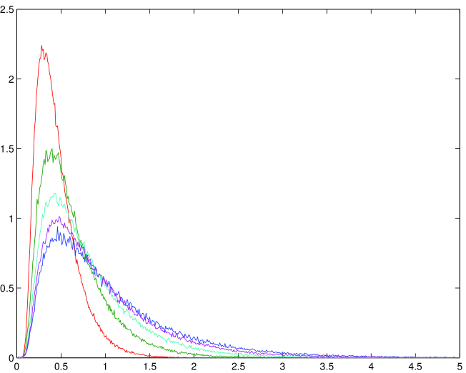
Figure 1: Estimated density of the first-passage area $A_{S}^{\mu}(x)$ of $X(t)=x+\mu t+B_{t}$ over $S,$ for $S=2,\ x=1$ and several values of $\mu.$ From top to bottom, with respect to the peak of the curve: $\mu=3;\ \mu=2;\ \mu=1.5;\ \mu=1.2;\ \mu=1.$

For some values of parameters we have compared the estimated density of the first-crossing area with a suitable Gamma density; in the Figure 2, we report for $S=2,\ x=1$ and $\mu=1.5,$ the comparison of the Laplace transform $M_{\lambda}(x)=E(e^{-\lambda A_{S}^{\mu}(x)})$ of the estimated first-crossing area density and the Laplace transform of the Gamma density with the same mean and variance. Although the two curves agree very well for small values of $\lambda>0$ (this implying a good agreement between the moments), for large values of $\lambda$ the graph of the Laplace transform of the estimated density of $A_{S}^{\mu}(x)$ lyes below the other one, which is compatible with an algebraic tail for the distribution of $A_{S}^{\mu}(x).$

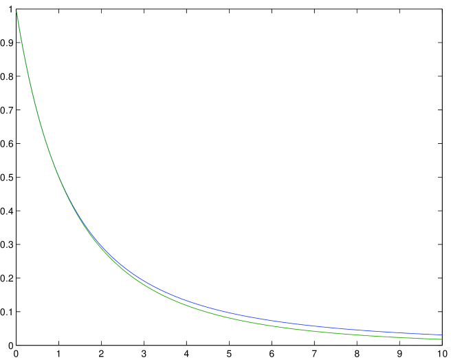
Figure 2: Comparison of the Laplace transform $M_{\lambda}(x)=E(e^{-\lambda A_{S}^{\mu}(x)})$ of the estimated density of the first-passage area $A_{S}^{\mu}(x)$ (lower curve) and the Laplace transform of the Gamma density with the same mean and variance (upper curve), as functions of $\lambda,$ for $S=2,\ x=1$ and $\mu=1.5.$

(iii) The distribution of the minimum $\mathfrak{m}^{\mu}(x).$

Set

$$\mathfrak{m}^{\mu}(x)=\min_{[0,\tau_{S}^{\mu}(x)]}\{x+\mu t+B_{t}\}.$$

Its distribution function $P(\mathfrak{m}^{\mu}(x)\leq z)=w(x)$ is the solution of the problem with boundary conditions:

$$\begin{cases}\frac{1}{2}w^{\prime\prime}(x)+\mu w^{\prime}(x)=0\\ w(z)=1,\ w(S)=0\end{cases}$$ (3.17)

By solving the above equation, we obtain, for $z\leq x:$

$$P(\mathfrak{m}^{\mu}(x)\leq z)=w(x)=\frac{e^{-2\mu x}-e^{2\mu S}}{e^{-2\mu z}-e^{-2\mu S}}$$ (3.18)

Then, calculating the derivative with respect to $z,$ we get the probability density of $\mathfrak{m}^{\mu}(x):$

$$f_{\mathfrak{m}^{\mu}(x)}(z)=\frac{2\mu e^{-2\mu z}\left(e^{-2\mu x}-e^{-2\mu S}\right)}{\left(e^{-2\mu z}-e^{-2\mu S}\right)^{2}}\ {\bf 1}_{(-\infty,x]}(z)$$ (3.19)

For $\mu=0,$ taking the limit in the above expression, we get $f_{\mathfrak{m}^{0}(x)}(z)=\frac{S-x}{(S-z)^{2}}\ {\bf 1}_{(-\infty,x]}(z),$ and so the moments of $\mathfrak{m}^{0}(x)$ of all orders $n\geq 1$ are infinite.

On the contrary, for $\mu>0$ the minimum $\mathfrak{m}^{\mu}(x)$ possesses finite moments of all orders, because $f_{\mathfrak{m}^{\mu}(x)}(z)$ behaves like $const/e^{-2\mu z},$ for $z\rightarrow-\infty.$

Definition 3.1

We say that a one-dimensional diffusion $X(t)$ with $X(0)=x,$ is conjugated to BM if there exists an increasing differentiable function $u(x),$ with $u(0)=0,$ such that $X(t)=u^{-1}\left(B_{t}+u(x)\right).$

Remark 3.2

If $X(t)$ is conjugated to Brownian motion via the function $u,$ then for $x<S:$

$$\tau_{S}(x)=\inf\{t>0:X(t)=S|X(0)=x\}=\inf\{t>0:u(X(t))=u(S)|u(X(0))=u(x)\}$$

$$=\inf\{t>0:B_{t}+u(x)=u(S)\}=\tau_{S^{\prime}}^{B}(u(x))$$

where $S^{\prime}=u(S)$ and $\tau_{S^{\prime}}^{B}(y)$ is the first hitting time to $S^{\prime}$ of $y+B_{t}$ (i.e. BM without drift starting from $y).$ Thus, the first-passage time through $S$ of the process $X(t)$ starting from $x<S,$ is nothing but the first hitting time to $S^{\prime}$ of BM starting from $u(x),$ and

$$A_{S}(x)=\int_{0}^{\tau_{S}(x)}X(t)dt=\int_{0}^{\tau_{S^{\prime}}^{B}(u(x))}u^{-1}(B_{t}+u(x))dt.$$

Notice that, though $\tau_{S}(x)$ turns out to be finite with probability one, it results $E(\tau_{S}(x))=+\infty.$ Moreover

$$M_{U,\lambda}(x)=E\left[\exp\left(-\lambda\int_{0}^{\tau_{S}(x)}U(X(t))dt\right)\right]=E\left[\exp\left(-\lambda\int_{0}^{\tau_{S^{\prime}}^{B}(u(x))}V(B_{t})dt\right)\right),$$

where $V(s)=U\left(u^{-1}(s+u(x))\right).$

Therefore, the Laplace transform $M_{U,\lambda}(x)$ of $\int_{0}^{\tau_{S}(x)}U(X(t))dt,$ associated to the functional $U$ of the process $X,$ is nothing but the Laplace transform $M_{V,\lambda}^{S^{\prime}}(y)$ of $\int_{0}^{\tau_{S^{\prime}}^{B}(y)}V(B_{t})dt,$ associated to the functional $V$ of BM, where $y=u(x).$

This means that the equation (3.4) is easily reduced to the analogous equation for BM starting from $u(x),$ with $U$ replaced by $V.$

Example 2.

A class of diffusions conjugated to BM is given by processes $X(t)$ which are solutions of SDEs such as

$$dX(t)=\frac{1}{2}\sigma(X(t))\sigma^{\prime}(X(t))dt+\sigma(X(t))dB_{t},\ X(0)=x_{0}$$ (3.20)

with $\sigma(\cdot)\geq 0.$ Indeed, if the integral $v(x)\doteq\int_{x_{0}}^{x}\frac{1}{\sigma(r)}dr$ is convergent for every $x,$ by It${\rm\hat{o}}$’s formula, we obtain that $X(t)=v^{-1}(B_{t}+v(x_{0})).$

(i)  (Feller process or Cox-Ingersoll-Ross (CIR) model)

For $a,b\geq 0,$ let $X(t)$ be the solution of the SDE

$$dX(t)=(a+bX(t))dt+\sqrt{X(t)\vee 0}\ dB_{t}\ ,X(0)=x_{0}\geq 0$$ (3.21)

(note that, although $\sqrt{x}$ is not Lipschitz-continuous, the solution is unique because $\sqrt{x}$ is H${\rm\ddot{o}}$lder-continuous of order $\frac{1}{2}$ (see condition A2)). The process $X(t)$ turns out to be non-negative for all $t\geq 0$ (see [7], [9]). If $b=0$ and $a=\frac{1}{4},$ the SDE (3.21) becomes:

$$dX(t)=\frac{1}{4}dt+\sqrt{X(t)\vee 0}\ dB_{t}\ ,X(0)=x_{0}$$

and $X(t)$ turns out to be conjugate to BM via the function $v(x)=2\sqrt{x}$ i.e. $X(t)=\frac{1}{4}(B_{t}+2\sqrt{x_{0}})^{2};$ the SDE is obtained by taking $\sigma(x)=\sqrt{x\vee 0}$ in (3.20).

(ii) (Wright & Fisher-like process).

The diffusion described by the SDE:

$$dX(t)=(a+bX(t))dt+\sqrt{X(t)(1-X(t))\vee 0}\ dB_{t},\ X(0)=x_{0}\in[0,1]$$ (3.22)

with $a\geq 0$ and $a+b\leq 0$ does not exit from the interval $[0,1]$ for any time (see [7], [9]). This equation is used for instance in the Wright-Fisher model for population genetics and in certain diffusion models for neural activity [22]. For $a=\frac{1}{4}$ and $b=-\frac{1}{2},$ $X(t)$ turns out to be conjugated to BM via the function $v(x)=2\arcsin\sqrt{x},$ i.e. $X(t)=\sin^{2}(B_{t}/2+\arcsin\sqrt{x_{0}}).$

For these special values of parameters, the SDE (3.22) becomes:

$$dX(t)=\left(\frac{1}{4}-\frac{1}{2}X(t)\right)dt+\sqrt{X(t)(1-X(t))}\ dB_{t}\ ,X(0)=x_{0}\in[0,1]$$

and it is obtained from (3.20) by taking $\sigma(x)=\sqrt{x(1-x)\vee 0}\ .$ Notice that, for $0\leq x<S\leq 1,$ it results $A_{S}(x)=\int_{0}^{\tau_{S}(x)}X(t)dt\leq\tau_{S}(x),$ since $0\leq X(t)\leq 1.$

Example 3 (Ornstein-Uhlenbeck process)

Let $X(t)$ be the solution of the SDE:

$$dX(t)=-\mu X(t)dt+\sigma dB_{t},\ X(0)=x$$ (3.23)

where $\mu$ and $\sigma$ are positive constants. By calculating the functions $\phi$ and $\xi$ in (3.2) and (3.3), we obtain:

$$\phi(x)=const\cdot\exp\left(\frac{\mu x^{2}}{\sigma^{2}}\right)$$

and

$$\xi(x)=const\cdot\frac{2}{\sigma}\sqrt{\frac{\pi}{\mu}}\exp\left(\frac{\mu x^{2}}{\sigma^{2}}\right)\left[\Phi\left(\frac{x\sqrt{2\mu}}{\sigma}\right)-\frac{1}{2}\right]$$

where $\Phi$ denotes the distribution function of the standard Gaussian variable. Since $\xi(x)$ is integrable in a neighbor of $x=S,$ the boundary $S$ is attainable.

The explicit solution of (3.23) is $X(t)=e^{-\mu t}\left(x+\int_{0}^{t}\sigma e^{\mu s}dB_{s}\right)$ (see e.g. [4], [6]). By using a time–change, we can write $\int_{0}^{t}\sigma e^{\mu s}dB_{s}=B_{\rho(t)},$ where $\rho(t)=\frac{\sigma^{2}}{2\mu}\left(e^{2\mu t}-1\right).$ Then, one gets $X(t)=e^{-\mu t}(x+B(\rho(t)).$ Let us consider e.g. the time dependent boundary $S(t)=H(t)=\alpha e^{-\mu t},$ then:

$$\tau_{H}(x)=\inf\{t>0:X(t)=H(t)|X(0)=x\}=\inf\{t>0:B(\rho(t))+x=\alpha\}$$

and so

$$\rho(\tau_{H}(x))=\inf\{s>0:x+B_{s}=\alpha\}=\tau_{\alpha}^{B}(x),$$

that is $\tau_{H}(x)=\rho^{-1}(\tau_{\alpha}^{B}(x)),$ where $\tau_{\alpha}^{B}(x)$ is the first-passage time through $\alpha$ of Brownian motion starting from $x.$ Thus, $\tau_{H}(x)$ has density

$$f_{\tau_{H}(x)}(t)=f_{\tau_{\alpha}^{B}(x)}(\rho(t))\rho^{\prime}(t)$$

where $f_{\tau_{\alpha}^{B}(x)}$ denotes the density of $\tau_{\alpha}^{B}(x),$ which is given by (3.9) with $\mu=0$ and $S=\alpha.$ Notice that even the mean of $\tau_{H}(x)$ is impractical to be directly calculated by using $f_{\tau_{H}(x)}(t).$

However, for a constant boundary $S$ it results (see e.g. [24]):

$$E(\tau_{S}(x))=\frac{1}{\mu}\big{\{}\sqrt{\pi}\left[\phi_{1}\left(S\sqrt{\mu}/\sigma\right)-\phi_{1}\left(x\sqrt{\mu}/\sigma\right)\right]+\psi_{1}\left(S\sqrt{\mu}/\sigma\right)-\psi_{1}\left(x\sqrt{\mu}/\sigma\right)\big{\}},$$

where

$$\phi_{1}(z)=\int_{0}^{z}e^{t^{2}}\ dt=\sum_{k=0}^{\infty}\frac{z^{2k+1}}{(2k+1)k!},$$

$$\psi_{1}(z)=2\int_{0}^{z}\ du\ e^{u^{2}}\int_{0}^{u}\ dv\ e^{-v^{2}}=\sum_{k=0}^{\infty}\frac{2^{k}}{(k+1)(2k+1)!!}z^{2k+2}.$$

Notice that, if $S>0,$ as seen by using Hospital’s rule, $\ E(\tau_{S}(x))$ tends to infinity, for $\mu\rightarrow 0,$ since the OU process reduces to BM; also for $\mu\rightarrow+\infty$ it tends to infinity, which is indeed natural, since the drift tends to $-\infty.$

As far as the minimum $\mathfrak{m}(x)$ is concerned, by Proposition 2.5 its distribution $w(x)=P(\mathfrak{m}(x)\leq z)$ satisfies the problem:

$$\begin{cases}\frac{1}{2}\sigma^{2}w^{\prime\prime}(x)-\mu xw^{\prime}(x)=0,\ z<x<S\\ w(z)=1,\ w(S)=0\end{cases}$$

whose solution is:

$$P(\mathfrak{m}(x)\leq z)=\left(\int_{x}^{S}e^{\frac{\mu}{\sigma^{2}}t^{2}}dt\right)\left(\int_{z}^{S}e^{\frac{\mu}{\sigma^{2}}t^{2}}dt\right)^{-1},\ z\leq x.$$

Thus, the density of $\mathfrak{m}(x)$ is:

$$\frac{d}{dz}P(\mathfrak{m}(x))\leq z)=\left[e^{\frac{\mu}{\sigma^{2}}z^{2}}\int_{x}^{S}e^{\frac{\mu}{\sigma^{2}}t^{2}}dt\left(\int_{z}^{S}e^{\frac{\mu}{\sigma^{2}}t^{2}}dt\right)^{-2}\right]\cdot{\bf 1}_{(-\infty,x]}(z).$$

3.2 Diffusions with jumps

Example 4 (Poisson process)

For $x>0,$ let us consider the jump-process $X(t)=x+N_{t},$ where $N_{t}$ is a homogeneous Poisson process with intensity $\theta>0,$ namely $N_{0}=0$ and its jumps, of amplitude $1,$ occur at independent instants, exponentially distributed with parameter $\theta.$ This means that

$$P(N_{t}=k)=\frac{e^{-\theta t}(\theta t)^{k}}{k!},\ {\rm for}\ k=0,1,\dots$$

The infinitesimal generator of the process is defined by:

$$Lg(x)=\theta[g(x+1)-g(x)],\ g\in C^{0}(\rm I\!R)$$

and, for $S>0$ and $x<S,$ $\tau_{S}(x)=\inf\{t>0:x+N_{t}\geq S\}.$

By Theorem 2.3 with $U(x)=1,$ it follows that the Laplace transform $M_{U,\lambda}(x)$ of $\tau_{S}(x)$ is the solution of the equation $LM_{U,\lambda}(x)=\lambda M_{U,\lambda}(x),$ with outer condition $M_{U,\lambda}(y)=1$ for $y\geq S.$ By solving this equation, we get:

$$M_{U,\lambda}(x)=\begin{cases}\left(\frac{\theta}{\theta+\lambda}\right)^{S-x}&{\rm if}\ S-x\in\rm I\!N\\ \left(\frac{\theta}{\theta+\lambda}\right)^{[S-x]+1}&{\rm if}\ S-x\notin\rm I\!N\end{cases}$$

where $[a]$ denotes the integer part of $a.$ Notice that the condition $M_{U,\lambda}(-\infty)=0$ also holds. Thus, recalling the expression of the Laplace transform of the Gamma density, we find that $\tau_{S}(x)$ has Gamma distribution with parameters $(S-x,\theta)$ if $S-x$ is a positive integer, while it has Gamma distribution with parameters $([S-x]+1,\theta)$ if $S-x$ is not an integer. This fact also follows directly, if one considers the nature of the Poisson process. The moments $T_{n}(x)=E\left[\tau_{S}^{n}(x)\right]$ are soon obtained from the density or also by the formula $T_{n}(x)=(-1)^{n}\left[\frac{\partial^{n}}{\partial\lambda^{n}}M_{U,\lambda}(x)\right]_{\lambda=0}.$ We have:

$$E(\tau_{S}(x))=\begin{cases}\frac{S-x}{\theta}&{\rm if}\ S-x\in\rm I\!N\\ \frac{[S-x]+1}{\theta}&{\rm if}\ S-x\notin\rm I\!N\end{cases}$$

and

$$E(\tau_{S}^{2}(x))=\begin{cases}\frac{(S-x)^{2}}{\theta^{2}}+\frac{S-x}{\theta^{2}}&{\rm if}\ S-x\in\rm I\!N\\ \frac{([S-x]+1)^{2}}{\theta^{2}}+\frac{[S-x]+1}{\theta^{2}}&{\rm if}\ S-x\notin\rm I\!N\end{cases}$$

Thus:

$$Var(\tau_{S}(x))=\begin{cases}\frac{S-x}{\theta^{2}}&{\rm if}\ S-x\in\rm I\!N\\ \frac{[S-x]+1}{\theta^{2}}&{\rm if}\ S-x\notin\rm I\!N\end{cases}$$

By Theorem 2.3 with $U(x)=x,$ we get the Laplace transform $M_{U,\lambda}(x)$ of $A_{S}(x)$ as the solution of the equation $LM_{U,\lambda}(x)=\lambda xM_{U,\lambda}(x),$ with outer condition $M_{U,\lambda}(y)=1$ for $y\geq S.$ By solving this equation, we get:

$$M_{U,\lambda}(x)=\begin{cases}\theta^{S-x}\cdot\{(\theta+\lambda x)(\theta+\lambda(x+1))\cdots(\theta+\lambda(x+(S-x)-1))\}^{-1}&{\rm if}\ S-x\in\rm I\!N\\ \theta^{[S-x]+1}\cdot\{(\theta+\lambda x)(\theta+\lambda(x+1))\cdots(\theta+\lambda(x+[S-x]))\}^{-1}&{\rm if}\ S-x\notin\rm I\!N\end{cases}$$

Notice that the condition $M_{U,\lambda}(-\infty)=0$ is fulfilled.

We observe that $M_{U,\lambda}(x)$ turns out to be the Laplace transform of a linear combination of $S-x$ independent exponential random variables with parameter $\theta,$ with coefficients $x,x+1,\dots,S-1,$   if $S-x$ is an integer, while it is the Laplace transform of a linear combination of $[S-x]+1$ independent exponential random variables with parameter $\theta,$ with coefficients $x,x+1,\dots,x+[S-x],$ if $S-x$ is not an integer.

The $n-$th order moment of $A_{S}(x)$ is given by $(-1)^{n}\left[\frac{\partial^{n}}{\partial\lambda^{n}}M_{U,\lambda}(x)\right]_{\lambda=0};$ calculating the first and second derivative, after some tedious computations, we obtain

$$E(A_{S}(x))=\begin{cases}\frac{S-x}{2\theta}(x+S-1)&{\rm if}\ S-x=k\in\rm I\!N\\ \frac{[S-x]+1}{2\theta}(2x+[S-x])&{\rm if}\ S-x\notin\rm I\!N\end{cases}$$

and

$$E(A_{S}^{2}(x))=\begin{cases}\frac{k}{12\theta^{2}}\{12x^{2}(k+1)+12x(k^{2}-1)+3k^{3}-2k^{2}-3k+2\}\ \ \ \ {\rm if}\ S-x=k\in\rm I\!N\\ \frac{[S-x]+1}{12\theta^{2}}\{12x([S-x]+2)(x+[S-x])+\\ +[S-x](3[S-x]^{2}+7[S-x]+2)\}\ \ \ \ \ \ \ \ \ \ \ \ \ \ \ \ \ \ \ \ \ \ \ \ \ \ \ \ \ \ \ \ \ {\rm if}\ S-x\notin\rm I\!N\end{cases}$$

Remark 3.3

Notice that

$$\tau_{S}(x)=\inf\{t>0:x+N_{t}\geq S\}=\inf\{t>0:S-x-N_{t}\leq 0\}=\widehat{\tau}(S-x)$$

where $\widehat{\tau}(y)$ is the first-passage time below zero of the process $Y(t):=y-N_{t}.$ Moreover, it holds $A_{S}(x)=S\tau_{S}(x)-\widehat{A}(S-x),$ where $\widehat{A}(y)$ is the area swept out by $Y(t)$ till its first passage below zero. Thus, the moments of $\tau_{S}$ and the mean of $A_{S}$ can be obtained by the moments of $\widehat{\tau}$ and $E(\widehat{A}),$ which were calculated in [2]. In this way, one can avoid the heavy computations above.

Example 5 (a Levy process)

Let us consider the process $X(t)=x+\beta t+B_{t}+N_{t},$ where $N_{t}$ is a homogeneous Poisson Process with intensity $\theta>0$ and let $S>0,\ \beta+\theta>S-x>0.$ We have $\tau_{S}(x)=\inf\{t>0:X(t)\geq S\}=\inf\{t>0:(S-x)-\beta t+W_{t}\leq N_{t}\}$ i.e. the first hitting time of BM $W_{t}$ with drift $-\beta$ starting from $S-x,$ and the Poisson process $N_{t}$ (see [10] as regards the density of $\tau_{S}(x))$ in a similar case). The condition $\beta+\theta>S-x$ assures that $\tau_{S}(x)$ is finite with probability one (see Remark 2.2). Now, the infinitesimal generator of the process is $Lf(x)=\frac{1}{2}f^{\prime\prime}(x)+\beta f^{\prime}(x)+f(x+1)-f(x)$ and the differential-difference equations involved to find the Laplace transforms of $\tau_{S}(x)$ and $A_{S}(x),$ as well as those for the moments of $\tau_{S}(x)$ and $A_{S}(x),$ cannot be solved explicitly; these quantities have to be found by a numerical procedure.

Remark 3.4

Until now we have supposed that the starting point $x<S$ is given and fixed. One could introduce a randomness in the starting point, replacing $X(0)=x$ with a random variable $\eta,$ having density $g(x)$ whose support is the interval $(-\infty,S).$ Thus, the quantities of interest become: $\tau_{S}=\inf\{t>0:X(t)>S\}$ and $A_{S}=\int_{0}^{\tau_{S}}X(t)dt,$ while $\tau_{S}(x)$ and $A_{S}(x)$ are the corresponding values conditional to $\eta=x.$ By using the found expressions for the moments of $\tau_{S}(x)$ and $A_{S}(x),$ one can easily calculate the moments of $\tau_{S}$ and $A_{S}.$ For instance, when $X(t)$ is BM with drift $\mu,$ it follows by (3.10) and (3.14) that:

$$E(\tau_{S}^{\mu})=\int_{-\infty}^{S}\frac{S-x}{\mu}\ g(x)dx=\frac{1}{\mu}E(S-\eta)$$

$$E((\tau_{S}^{\mu})^{2})=\int_{-\infty}^{S}\left(\frac{S-x}{\mu^{3}}+\frac{(S-x)^{2}}{\mu^{2}}\right)\ g(x)dx=\frac{1}{\mu^{3}}E(S-\eta)+\frac{1}{\mu^{2}}E((S-\eta)^{2})$$

$$E(A_{S}^{\mu})=\int_{-\infty}^{S}\frac{S-x}{2\mu}\left(S+x-\frac{1}{\mu}\right)\ g(x)dx=\frac{1}{2\mu}E\left[\left(S-\eta\right)\left(S+\eta-\frac{1}{\mu}\right)\right].$$

4 Conclusions and Final Remarks

For $S>0,$ we have considered a one-dimensional jump-diffusion process $X(t)$ starting from $x<S,$ that is, a diffusion to which jumps at Poisson-distributed instants are superimposed; then, we have studied the probability distribution of the (random) area $A_{S}(x)=\int_{0}^{\tau_{S}(x)}X(t)dt$ swept out by $X(t)$ till its first-passage time over the barrier $S,$ i.e. the (random) time $\tau_{S}(x)=\inf\{t>0:X(t)\geq S|X(0)=x\}.$ The analogous problem concerning the first passage of $X(t)$ below zero was studied in [2], while results for Brownian motion with negative drift were obtained e.g. in [16], [18], [19], [21], [23].

In particular, we have shown that the Laplace transforms of $A_{S}(x)$ and $\tau_{S}(x),$ their moments, as well as the probability distribution of the minimum of $X(t)$ in $[0,\tau_{S}(x)],$ are solutions to certain partial differential-difference equations (PDDEs) with outer conditions. Notice that, in the absence of jumps, these PDDEs with outer conditions become simply PDEs with boundary conditions. The quantities here investigated have interesting applications in Queueing Theory and in Economics (see the Introduction for a brief discussion).

After considering theoretical results for diffusions $X(t)$ with and without jumps, in the final part of the paper we reported some examples for which we have carried out explicit calculations. We remark that, in general it is not possible to solve explicitly the equations involved, in order to find closed formulae for the Laplace transform of the first-crossing area, and for its moments; moreover, even if one is able to find explicitly the Laplace transform, it is not always possible to invert it, to get the distribution of $A_{S}(x).$

When the analytical solution is not available, due to the complexity of calculations, one can resort to numerical solution of the PDDEs involved; alternatively, one can carry out computer simulation of a large enough number of trajectories of the process $X(t),$ in order to obtain statistical estimations of the quantities of interest.

References

• [1] Abramowitz, M.; Stegun, I. A. Handbook of Mathematical Functions with Formulas, Graphs, and Mathematical Tables. Dover, New York, 1965
• [2] Abundo, M. On the first-passage area of one-dimensional jump-diffusion process. Methodol. Comput. Appl. Probab. Online First 2011, DOI: 10.1007/s11009-011-9223-1.
• [3] Abundo, Marco; Abundo, Mario On the first-passage area of an emptying Brownian queue. International Journal of Applied Mathematics (IJAM) 2011, 24 (2), 259–266.
• [4] Abundo, M. First-Passage Problems for Asymmetric Diffusions and Skew-diffusion Processes. Open Systems $\&$ Information Dynamics 2009, 16 (4), 325–350.
• [5] Abundo, M. On the distribution of the time average of a jump-diffusion process. International Journal of Applied Mathematics 2008, 21 (3), 447–454.
• [6] Abundo, M. On first-passage problems for asymmetric one-dimensional diffusions. Lecture Notes in Computer Science, Computer Aided Systems Theory - EUROCAST 2007; 4739, 179–186. Springer Berlin/ Heidelberg, 2007.
• [7] Abundo, M. Limit at zero of the first-passage time density and the inverse problem for one-dimensional diffusions. Stochastic Anal. Appl. 2006, 24, 1119–1145.
• [8] Abundo, M. On first-passage-times for one-dimensional jump-diffusion processes. Prob. Math. Statis. 2000, 20 (2), 399–423.
• [9] Abundo, M. On some properties of one-dimensional diffusion processes on an interval. Prob. Math. Statis. 1997, 17 (2), 235–268.
• [10] Abundo, M. On the First Hitting Time of a One-dimensional Diffusion and a Compound Poisson Process. Methodol. Comput. Appl. Probab. 2010, 12, 473–490
• [11] Darling, D. A.; Siegert, A.J.F. The first passage problem for a continuous Markov process. Ann. Math. Statistics 1953, 24, 624–639.
• [12] Gihman, I.I.; Skorohod, A.V. Stochastic differential equations. Springer-Verlag, Berlin, 1972.
• [13] Grandshteyn, I.S.; Ryzhik, I. M. Tables of Integrals, Series and Products. 5th ed. Academic, London, 1980.
• [14] Has’ minskij, R.Z. Stochastic stability of differential equations. Alphen a/d Rijn, Sijthoff $\&$ Noordhoff, 1980
• [15] Ikeda, N.; Watanabe, S. Stochastic differential equations and diffusion processes. North-Holland Publishing Company, 1981
• [16] Janson, S. Brownian excursion area, Wright s constants in graph enumeration, and other Brownian areas. Probability Surveys 2007, 4, 80–145.
• [17] Karlin, S.; Taylor, H.M. A second course in stochastic processes. Academic Press, New York, 1975.
• [18] Kearney, M. J.; Majumdar, S.N. On the area under a continuous time Brownian motion till its first-passage time. J. Phys. A: Math. Gen. 2005, 38; 4097–4104.
• [19] Kearney, M. J.; Majumdar, S.N.; Martin R.J. The first-passage area for drifted Brownian motion and the moments of the Airy distribution. J. Phys. A: Math. Theor. 2007, 40, F863–F864.
• [20] Klebaner, F. C. Β Introduction to stochastic calculus with applications. Imperial College Press, Singapore, 1999.
• [21] Knight, F. B. The moments of the area under reflected Brownian Bridge conditional on its local time at zero. Journal of Applied Mathematics and Stochastic Analysis 2000, 13 (2), 99–124.
• [22] Lanska, V.; Lansky, P.; Smiths, C.E. Synaptic transmission in a diffusion model for neural activity. J. Theor. Biol. 1994, 166, 393–406.
• [23] Perman, M.; Wellner, J. A. On the Distribution of Brownian Areas. The Annals of Applied Probability 1996, 6 (4), 1091–1111.
• [24] Ricciardi, L.M; Di Crescenzo, A.; Giorno V.; Nobile, A.G. An outline of theoretical and algorithmic approaches to first passage time problems with applications to biological modeling. Math. Japonica 1999, 50 (2), 247–322.
• [25] Tuckwell, H.C. On the first exit time problem for temporally homogeneous Markov processes. The Annals of Applied Probability 1976, 13, 39–48.