Convex Relaxations for Learning Bounded Treewidth Decomposable Graphs

Abstract

We consider the problem of learning the structure of undirected graphical models with bounded treewidth, within the maximum likelihood framework. This is an NP-hard problem and most approaches consider local search techniques. In this paper, we pose it as a combinatorial optimization problem, which is then relaxed to a convex optimization problem that involves searching over the forest and hyperforest polytopes with special structures, independently. A supergradient method is used to solve the dual problem, with a run-time complexity of $O(k^{3}n^{k+2}\log n)$ for each iteration, where $n$ is the number of variables and $k$ is a bound on the treewidth. We compare our approach to state-of-the-art methods on synthetic datasets and classical benchmarks, showing the gains of the novel convex approach.

1 Introduction

Graphical models provide a versatile set of tools for probabilistic modeling of large collections of interdependent variables. They are defined by graphs that encode the conditional independences among the random variables, together with potential functions or conditional probability distributions that encode the specific local interactions leading to globally well-defined probability distributions [4, 32, 16].

In many domains such as computer vision, natural language processing or bioinformatics, the structure of the graph follows naturally from the constraints of the problem at hand. In other situations, it might be desirable to estimate this structure from a set of observations. It allows (a) a statistical fit of rich probability distributions that can be considered for further use, and (b) discovery of structural relationship between different variables. In the former case, distributions with tractable inference are often desirable, i.e., inference with run-time complexity does not scale exponentially in the number of variables in the model. The simplest constraint to ensure tractability is to impose tree-structured graphs [7]. However, these distributions are not rich enough, and following earlier work [21, 1, 22, 6, 13, 29], we consider models with bounded treewidth, not simply by one (i.e., trees), but by a small constant $k$.

Beyond the possibility of fitting tractable distributions (for which probabilistic inference has linear complexity in the number of variables), learning bounded-treewidth graphical models is a key to design approximate inference algorithms for graphs with higher treewidth. Indeed, as shown by [24, 32, 17], approximating general distributions by tractable distributions is a common tool in variational inference. However, in practice, the complexity of variational distributions is often limited to trees (i.e., $k=1$), since these are the only ones with exact polynomial-time structure learning algorithms. The convex relaxation designed in this paper enables us to augment the applicability of variational inference, by allowing a finer trade-off between run-time complexity and approximation quality.

Apart from trees, learning the structure of a directed or undirected graphical model, with or without constraints on the treewidth, remains a hard problem. Two types of algorithms have emerged, based on the two equivalent definitions of graphical models: (a) by testing conditional independence relationships [27] or (b) by maximizing the log-likelihood of the data using the factorized form of the distribution [11]. In the specific context of learning bounded-treewidth graphical models, the latter approach has been shown to be NP-hard [28] and led to various approximate algorithms based on local search techniques [21, 9, 15, 1, 26, 29] while the former approach led to algorithms based on independence tests [22, 6, 13], which have recovery guarantees when the data-generating distribution has low treewidth. Malvestuto [21] proposed a greedy heuristic of hyperedge selection with least incremental entropy. Deshpande et al. [9] proposed a simple edge selection technique that maintains decomposability of the graph while minimizing the KL-divergence to the original distribution. Karger et al. [15] proposed the first convex optimization approach to learn the maximum weighted $k$-windmill, a sub-class of the decomposable graph. Bach et al. [1] gave an approach which iteratively refines the hyperedge selection based on KL-divergence using iterative scaling. Shahaf et al. [26] proposed another convex optimization approach with Bethe approximation of the likelihood using graph-cuts. Szántai et al. [29] proposed a hyperedge selection criteria based on high mutual information within a hyperedge. Narasimhan et al. [22] performs independence tests by solving submodular optimization problems and derives a decomposable graph using dynamic programming. Chechetka et al. [6] used the weaker notion of conditional mutual information instead of conditional independence to learn approximate junction trees. Gogate et al. [13] uses low mutual information criteria to recursively split the state space to smaller subsets until no further splits are possible.

In this paper, we make the following contributions:

• We provide a novel convex relaxation for learning bounded-treewidth decomposable graphical models from data in polynomial time. This is achieved by posing the problem as a combinatorial optimization problem in Section 2, which is relaxed to a convex optimization problem that involves the graphic and hypergraphic matroids, as shown in Section 3.

• We show in Section 4 how a supergradient ascent method may be used to solve the dual optimization problem, using greedy algorithms as inner loops on the two matroids. Each iteration has a run-time complexity of $O(k^{3}n^{k+2}\log n)$, where $n$ is the number of variables. We also show how to round the obtained fractional solution.

• We compare our approach to state-of-the-art methods on synthetic datasets and classical benchmarks in Section 5, showing the gains of the novel convex approach.

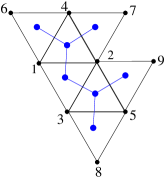
(a)	(b)	(c)

Figure 1: (a) A decomposable graph on the set of vertices $V=\{1,2,3,4,5,6,7,8,9\}$ having treewidth 2.(b) A junction tree embedded on the decomposable graph representing the maximal cliques by blue dots and the separator sets by blue lines. (c) The corresponding junction tree representation of the decomposable graph with ovals representing the maximal cliques and the rectangles representing the corresponding separator set.

2 Maximum Likelihood Decomposable Graphical Models

In this section, we first review the relevant concepts of decomposable graphs and junction trees; for more details, see [4, 32, 16]. We then cast the problem of learning the maximum likelihood bounded treewidth graph as a combinatorial optimization problem.

2.1 Decomposable graphs and junction trees

We assume we are given an undirected graph $G$ defined on the set of vertices $V=\{1,2,\ldots,n\}$. Let $\mathcal{C}(G)$ denote the set of maximal cliques of $G$ (which we will refer to as cliques). We consider $n$ random variables $X_{1},\dots,X_{n}$ (referred to as $X$), associated with each vertex indexed by $V$. For simplicity, they are assumed to be discrete, but this is not a restriction as maximum likelihood will use only entropies that can be extended to differentiable entropies [8].

The distribution $p(x)$ of $X$ is said to factorize in the graph $G$, if and only if it factorizes as a product of potentials that depend only on the variables within maximal cliques.

A graph is said to be decomposable if it has a junction tree, i.e., a spanning tree whose vertices are maximal cliques of $G$ (i.e., $\mathcal{C}(G)$ is the vertex set) such that:

• the junction tree connects only cliques that have a common element (clique tree property),

• for any vertex $i\in V$, the subgraph of cliques containing $i$ is a tree (running intersection property).

Let $\mathcal{T}(G)$ denote the edges of the junction tree over the set of cliques $\mathcal{C}(G)$. When the graph $G$ is decomposable, the distribution $p(x)$ of $X$ factorizes in $G$ if and only if it may be written as

$$p_{G}(x)=\frac{\prod_{C\in\mathcal{C}(G)}p_{C}(x_{C})}{\prod_{(C,D)\in\mathcal{T}(G)}p_{C\cap D}(x_{C\cap D})}\text{ ,}$$ (1)

where $x$ is an instance in the domain of $X$, which we denote by $\mathcal{X}$. $p_{C}(x_{C})$ denotes the marginal distribution of random variables belonging to $C\in\mathcal{C}(G)$ and $p_{C\cap D}(x_{C\cap D})$ denotes the marginal distribution of random variables belonging to the separator set $C\cap D$, such that $(C,D)\in\mathcal{T}(G)$. See Figure 1. The treewidth of $G$ is the maximal size of the cliques in $G$, minus one.

An alternative representation of decomposable graphs may be obtained by considering hypergraphs. Hypergraphs are defined by a base set $V$ and a set of hyperedges, i.e., subsets of $V$. A hypergraph is said to be acyclic if and only if the resulting graph obtained by connecting all elements within an hyperedge is decomposable. Unfortunately, the nice properties of acyclic graphs do not transfer to acyclic hypergraphs. Particulary, the matroid property, which allows exact greedy algorithms, does not hold. In Section 3.2, we will use a lesser known more general notion of acyclicity that will lead to exact greedy algorithms.

2.2 Maximum likelihood estimation

Given $N$ observations $x^{1},\dots,x^{N}$ of $X$, we denote the corresponding empirical distribution of $X$ by $\hat{p}(x)=\frac{1}{N}\sum_{i=1}^{N}\delta(x=x^{i})$. Given the structure of a decomposable graph $G$, the maximum likelihood distribution that factorizes in $G$ may be obtained by combining the marginal empirical distributions on all maximum cliques and their separators.

Let $\hat{p}(x)$ denote the empirical distribution and $\hat{p}_{G}(x)$ denotes the projected distribution on a decomposable graph $G$. Estimating the maximum likelihood decomposable graph which best approximates $\hat{p}$ is equivalent to finding the graph, $G$, which minimizes the KL-divergence between the target distribution and the projected distribution, $\hat{p}_{G}$, defined by $D(\hat{p}||\hat{p}_{G})$.

$$D(\hat{p}||\hat{p}_{G}) = \sum_{x\in\mathcal{X}}\hat{p}(x)\log\frac{\hat{p}(x)}{\hat{p}_{G}(x)}$$ (2)

$$\propto \sum_{x\in\mathcal{X}}-\hat{p}(x)\log\hat{p}_{G}(x)\text{ as $\hat{p}(x)$ is independent of $G$ }$$

$$= \sum_{x\in\mathcal{X}}-\hat{p}(x)\log\frac{\prod_{C\in\mathcal{C}(G)}\hat{p}_{C}(x_{C})}{\prod_{(C,D)\in\mathcal{T}(G)}\hat{p}_{C\cap D}(x_{C\cap D})}\text{ from Eq.~{}(\ref{eq:jpd}) }$$

$$= \sum_{x\in\mathcal{X}}\bigg{(}-\hat{p}(x)\log\prod_{C\in\mathcal{C}(G)}\hat{p}_{C}(x_{C})\bigg{)}-\sum_{x\in X}\bigg{(}-\hat{p}(x)\log\prod_{(C,D)\in\mathcal{T}(G)}\hat{p}_{C\cap D}(x_{C\cap D})\bigg{)}$$

$$= \sum_{C\in\mathcal{C}(G)}\sum_{x\in\mathcal{X}}-\hat{p}(x)\log\hat{p}_{C}(x_{C})-\sum_{(C,D)\in\mathcal{T}(G)}\sum_{x\in\mathcal{X}}-\hat{p}(x)\log\hat{p}_{C\cap D}(x_{C\cap D})$$

$$= \sum_{C\in\mathcal{C}(G)}\sum_{x_{C}\in\mathcal{X}_{C}}-\hat{p}_{C}(x_{C})\log\hat{p}_{C}(x_{C})-\sum_{(C,D)\in\mathcal{T}(G)}\sum_{x_{C\cap D}\in\mathcal{X}_{C\cap D}}-\hat{p}_{C\cap D}(x_{C\cap D})\log\hat{p}_{C\cap D}(x_{C\cap D})$$

$$= \sum_{C\in\mathcal{C}(G)}H(C)-\sum_{(C,D)\in\mathcal{T}(G)}H({C\cap D})\text{ ,}$$

where $H(S)$ is the empirical entropy of the random variables indexed by the set $S\subseteq V$, defined by $H(S)=\sum_{x_{S}}\{-\hat{p}_{S}(x_{S})\log\hat{p}_{S}(x_{S})\}$, and where the sum is taken over all possible values of $x_{S}$.

Note that in this paper, we will not be using a traditional model selection term [11] as we will only consider models of low tree-width (with a bounded number of parameters).

2.3 Combinatorial optimization problem

We now consider the problem of learning a decomposable graph of treewidth less than $k$. We assume that we are given all entropies $H(S)$ for subsets $S$ of $V$ of cardinality less than $k+1$.

Since we do not add any model selection term, without loss of generality [30], we restrict the search space to the space of maximal junction trees, i.e., junction trees with $n-k$ maximal cliques of size $k+1$ and $n-k-1$ separator sets of size $k$ between two cliques of size $k+1$. Our natural search spaces are thus characterized by $\mathcal{D}$, the set of all subsets of size $k+1$ of $V$, of cardinality ${n\choose k+1}$, and $\mathcal{E}$, the set of all potential edges in a junction tree, i.e., $\mathcal{E}=\{(C,D)\in\mathcal{D}\times\mathcal{D},C\cap D\neq\varnothing,|C\cap D|=k\}$. The cardinality of $\mathcal{E}$ is ${n\choose k+2}.{k+2\choose 2}$ (number of subsets of size $k+2$ times the number of possibility of excluding two elements to obtain a separator).

A decomposable graph will be represented by a clique selection function $\tau:\mathcal{D}\to\{0,1\}$ and an edge selection function $\rho:\mathcal{E}\to\{0,1\}$ so that $\tau(C)=1$ if $C$ is a maximal clique of the graph and $\rho(C,D)=1$ if $(C,D)$ is an edge in the junction tree. Both $\rho$ and $\tau$ will be referred to as incidence functions or incidence vectors, when seen as elements of $\{0,1\}^{\mathcal{D}}$ and $\{0,1\}^{\mathcal{E}}$.

Thus, minimizing the problem defined in Eq. (2) is equivalent to minimizing,

$$\mathcal{P}(\tau,\rho)\!=\!\sum_{C\in\mathcal{D}}H(C)\tau(C)-\!\!\!\!\sum_{(C,D)\in\mathcal{E}}\!\!\!\!H(C\cap D)\rho(C,D),$$ (3)

with the constraint that $(\tau,\rho)$ forms a decomposable graph.

At this time, we have merely reparameterized the problem with the clique and edge selection functions. We now consider a set of necessary and sufficient conditions for the pair to form a decomposable graph. Some are convex in $(\tau,\rho)$, while some are not. The latter ones will be relaxed in Section 3. From now on, we denote by $1_{i\in C}$ the indicator function for $i\in C$ (i.e., it is equal to 1 if $i\in C$ and zero otherwise).

• Covering $V$: Each vertex in $V$ must be covered by atleast one of the selected cliques,

  $$\forall i\in V,\ \sum_{C\in\mathcal{D}}1_{i\in C}\tau(C)\geq 1.$$ (4)

• Number of edges: Exactly $n-k-1$ edges from $\mathcal{E}$ must be selected,

  $$\sum_{(C,D)\in\mathcal{E}}\rho(C,D)=n-k-1.$$ (5)

• Number of cliques: Exactly $n-k$ cliques from $\mathcal{D}$ must be selected,

  $$\sum_{C\in\mathcal{D}}\tau(C)=n-k.$$ (6)

• Running intersection property: Every vertex, $i\in V$ must induce a tree, i.e., the number of selected edges containing the vertex, $i$, must be equal to the number of selected cliques containing the vertex, $i$ , minus one.

  $$\!\!\!\!\!\!\forall i\in V,\sum_{(C,D)\in\mathcal{E}}\!\!1_{i\in(C\cap D)}\rho(C,D)-\sum_{C\in\mathcal{D}}1_{i\in C}\tau(C)+1=0.$$ (7)

• Edges between selected cliques: An edge in $\mathcal{E}$ is selected by $\rho$ only if the cliques it is incident on is selected by $\tau$.

  $$\forall C\in\mathcal{D},\ \tau(C)=\max_{D\in\mathcal{D},\ (C,D)\in\mathcal{E}}\rho(C,D).$$ (8)

• Acyclicity of $\rho$: $\rho$ selects edges in $\mathcal{E}$ such that they do not have loops, e.g., the blue lines in Figure 1-(b) cannot form loops,

  $$\rho (\mathcal{D},\mathcal{E})$$ represents a subforest of the graph . (9)

• Acyclicity of $\tau$: $\tau$ selects the hyperedges of $V$ in $\mathcal{D}$ such that they are acyclic, i.e.,

  $$\tau (V,\mathcal{D})$$ represents an acyclic hypergraph of . (10)

The above constraints encode the classical definition of junction trees. Thus our combinatorial problem is exactly equivalent to minimizing $P(\tau,\rho)$ defined in Eq. (3), subject to the constraints in in Eq. (4), Eq. (5), Eq. (6), Eq. (7), Eq. (8), Eq. (9) and Eq. (10). Note that the constraint Eq. (10) that $\tau$ represents an acyclic hypergraph is implied by the other constraints.

Figure 2 shows clique and edge selections in blue which satisfy all these constraints and hence represent a decomposable graph. The clique and edge selections in red violates at least one of these constraints.

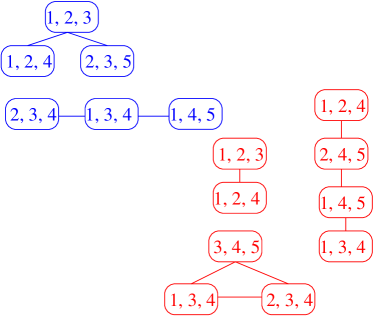
Figure 2: Space of cliques $\mathcal{D}$ denoted by ovals and the space of feasible edges $\mathcal{E}$ denoted by lines for $V=\{1,2,3,4,5\}$ and treewidth 2(in Black). Clique and edge selections in blue represent decomposable graphs while those in red denote graphs that are not decomposable (best seen in color).

3 Convex Relaxation

We now provide a convex relaxation of the combinatorial problem defined in Section 2.3. The covering constraint in Eq. (4), the number of edges and the number of cliques constraints in Eq. (5) and Eq. (6) respectively, and the running intersection property in Eq. (7) are already convex in $(\tau,\rho)$.

The constraint in Eq. (8) that $\forall C\in\mathcal{D},\ \tau(C)=\max_{D\in\mathcal{D},\ (C,D)\in\mathcal{E}}\rho(C,D)$ may be relaxed into:

• Edge constraint: selection of edges only if the both the incident cliques are selected, i.e.,

  $$\forall C\in\mathcal{D},\ \forall(C,D)\in\mathcal{E},\ \rho(C,D)\leq\tau(C).$$ (11)

• Clique constraint: selection of a clique if at least an edge incident on it is selected, i.e.,

  $$\forall C\in\mathcal{D},\ \tau(C)\leq\sum_{(C,D)\in\mathcal{E}}\rho(C,D).$$ (12)

We now consider the two acyclicity constraints in Eq. (9) and Eq. (10).

3.1 Forest polytope

Given the graph $(\mathcal{D},\mathcal{E})$, the forest polytope is the convex hull of all incidence vectors $\rho$ of subforests of $(\mathcal{D},\mathcal{E})$. Thus, it is exactly the convex hull of all $\rho:\mathcal{E}\to\{0,1\}$ such that $\rho$ satisfies the constraint in Eq. (9). We may thus relax it into:

• Tree constraint:

  $$\rho (\mathcal{D},\mathcal{E})$$ is in the forest polytope of . (13)

While the new constraint in Eq. (13) forms a convex constraint, it is crucial that it may be dealt with empirically in polynomial time. This is made possible by the fact that one may maximize any linear function over that polytope. Indeed, for a weight function $w:\mathcal{E}\times\mathcal{E}\to\mathbb{R}$, maximizing $\sum_{(C,D)\in\mathcal{E}}w(C,D)\rho(C,D)$ is exactly a maximum weight spanning forest problem, and its solution may be obtained by Kruskal’s algorithm, i.e., (a) order all (potentially negative) weights $w(C,D)$ and (b) greedily select edges $(C,D)$, i.e., set $\rho(C,D)=1$, with higher weights first, as long as they form a forest and as long as the weights are positive. When we add the restriction that the number of edges is fixed (in our case $n-k-1$), then the algorithm is stopped when exactly the desired number of edges is selected (whether the corresponding weights are positive or not). See, e.g., [25].

The polytope defined above may also be defined as the independence polytope of the graphic matroid, which is the traditional reason why the greedy algorithm is exact [25]. In the next section, we show how this can be extended to hypergraphs.

3.2 Hypergraphic matroid

Given the set of potential cliques $\mathcal{D}$ over $V$, we consider functions $\tau:\mathcal{D}\to\{0,1\}$ that are equal to one when a clique is selected, and zero otherwise. Ideally, we would like to treat the acyclicity of the associated hypergraph in a similar way than for regular graphs. However, the set of acyclic subgraphs of the hypergraph defined from $\mathcal{D}$ does not form a matroid, and thus the polytope defined as the convex hull of all incidence vectors/functions of acyclic hypergraphs may be defined, but the greedy algorithm is not applicable. In order to define what is referred to as the hypergraphic matroid, one needs to relax the notion of acyclicity.

We now follow [20, 10, 12] and define a different notion of acyclicity for hypergraphs. An hypergraph $(V,\mathcal{F})$ is an hyperforest if and only if for all $A\subset V$, the number of hyperedges in $\mathcal{F}$ contained in $A$ is less than $|A|-1$. A non-trivially equivalent definition is that we can select two elements in each hyperedege so that the graph with vertex set $V$ and with edge set composed of these pairs is a forest.

Given an hypergraph with hyperedge set $\mathcal{D}$, the set of sub-hypergraphs which are hyperforests forms a matroid. This implies that given a weight function on $\mathcal{D}$, one may find the maximum weight hyperforest with a greedy algorithm that ranks all hyperedges and select them as long as they don’t violate acyclicity (with the notion of acyclicity just defined and for which we exhibit a test below).

Testing acyclicity.

Checking acyclicity of an hypergraph $(V,\mathcal{F})$ (which is needed for the greedy algorithm above) may be done by minimizing with respect to $A\subset V$

$$|A|-\sum_{G\in\mathcal{F}}1_{G\subset A}.$$

The hypergraph is an hyperforest if and only if the minimum is greater or equal to one. The minimization of this function may be cast a min-cut/max-flow problem as follows [12]:

• single source, single sink, one node per hyperedge in $\mathcal{F}$, one node per vertex in $V$,

• the source points towards each hyperedge with unit capacity,

• each hyperedge points towards the vertices it contains, with infinite capacity,

• each vertex points towards the sink, with unit capacity.

Link with decomposability.

The hypergraph obtained from the maximal cliques of a decomposable graph can easily be seen to be an hyperforest. But the converse is not true.

Hyperforest polytope.

We can now naturally define the hyperforest polytope as the convex hull of all incidence vectors of hyperforests. Thus the constraint in Eq. (10) may be relaxed into:

• Hyperforest constraint:

  $$\tau (V,\mathcal{D})$$ is in the hyperforest polytope of . (14)

3.3 Relaxed optimization problem

We can now formulate our combinatorial problem from the constraints in Eq. (4), Eq. (5), Eq. (6), Eq. (7), Eq. (11), Eq. (12), Eq. (13) and Eq. (14) as follows

$$\min\mathcal{P}(\tau,\rho)\text{ subject to }\left\{\begin{array}[]{l}\tau\in\{0,1\}^{\mathcal{D}},\\ \rho\in\{0,1\}^{\mathcal{E}},\\ \forall i\in V,\sum_{C\in\mathcal{D}}1_{i\in C}\tau(C)\geq 1,\\ \sum_{(C,D)\in\mathcal{E}}\rho(C,D)=n-k-1,\\ \sum_{C\in\mathcal{D}}\tau(C)=n-k,\\ \forall i\in V,\sum_{(C,D)\in\mathcal{E}}1_{i\in(C\cap D)}\rho(C,D)-\sum_{C\in\mathcal{D}}1_{i\in C}\tau(C)+1=0,\\ \forall C\in\mathcal{D},\forall(C,D)\in\mathcal{E},\rho(C,D)\leq\tau(C),\\ \forall C\in\mathcal{D},\tau(C)\leq\sum_{(C,D)\in\mathcal{E}}\rho(C,D),\\ \text{$\rho$ is in the forest polytope of $(\mathcal{D},\mathcal{E})$},\\ \text{$\tau$ is in the hyperforest polytope of $(V,\mathcal{D})$.}\end{array}\right.$$ (15)

All constraints except the integrality constraints are convex. Let $\tau$-relaxed primal be the partially relaxed primal optimization problem formed by relaxing only the integral constraint on $\tau$ in Eq. (15), i.e., replacing $\tau\in\{0,1\}^{\mathcal{D}}$ by $\tau\in[0,1]^{\mathcal{D}}$. Note that this is not a convex problem due to the remaining integral constraint on $\rho$, but it remains equivalent to the original problem as the following proposition shows.

Proposition 1

The combinatorial problem in Eq. (15) and the $\tau$-relaxed primal problem are equivalent.

Proof  Let us assume $(\tau^{*},\rho^{*})$ be a feasible solution for the relaxed primal with $0<\tau^{*}(C)<1$ for some $C\in\mathcal{D}$. The edge constraint in Eq. (11) ensures that there are no incident edges on $C$ selected by $\rho^{*}$ (as $\rho^{*}$ is integral). This violates the clique constraint in Eq. (12). Therefore, the feasible solutions of relaxed primal are integral. Hence the optimal solutions of the primal and the relaxed primal are identical.  

The convex relaxation for the primal optimization problem formed by relaxing the integral constraint on both $\tau$ and $\rho$ can now be defined as

$$\min\mathcal{P}(\tau,\rho)\text{ subject to }\left\{\begin{array}[]{l}\tau\in[0,1]^{\mathcal{D}},\\ \rho\in[0,1]^{\mathcal{E}},\\ \forall i\in V,\sum_{C\in\mathcal{D}}1_{i\in C}\tau(C)\geq 1,\\ \sum_{(C,D)\in\mathcal{E}}\rho(C,D)=n-k-1,\\ \sum_{C\in\mathcal{D}}\tau(C)=n-k,\\ \forall i\in V,\sum_{(C,D)\in\mathcal{E}}1_{i\in(C\cap D)}\rho(C,D)-\sum_{C\in\mathcal{D}}1_{i\in C}\tau(C)+1=0,\\ \forall C\in\mathcal{D},\forall(C,D)\in\mathcal{E},\rho(C,D)\leq\tau(C),\\ \forall C\in\mathcal{D},\tau(C)\leq\sum_{(C,D)\in\mathcal{E}}\rho(C,D),\\ \text{$\rho$ is in the forest polytope of $(\mathcal{D},\mathcal{E})$},\\ \text{$\tau$ is in the hyperforest polytope of $(V,\mathcal{D})$.}\end{array}\right.$$ (16)

4 Solving the dual problem

We now show how the convex problem may be minimized in polynomial time. Among the constraints of our convex problem in Eq. (15), some are simple linear constraints, some are complex constraints depending on the forest and hyperforest polytopes defined in Section 3. We will define a dual optimization problem by introducing the least possible number of Lagrange multipliers (a.k.a. dual variables) [3] so that the dual function (and a supergradient) may be computed and maximized efficiently. We introduce the following dual variables:

• Set cover constraints in Eq. (4): $\gamma\in\mathbb{R}_{+}^{V}$.

• Running intersection property in Eq. (7): $\mu\in\mathbb{R}^{V}$.

• Edge constraints in Eq. (11): $\lambda\in\mathbb{R}_{+}^{2\mathcal{E}}$.

• Clique constraints in Eq. (12): $\eta\in\mathbb{R}_{+}^{\mathcal{D}}$.

Therefore, the dual variables are $(\gamma,\mu,\lambda,\eta)$. Let $\mathcal{L}(\tau,\rho,\gamma,\mu,\lambda,\eta)$ be the Lagrangian relating the primal and dual variables. It is derived from the primal cost function defined in Eq. (3) along with the covering constraint, running intersection property, the edge and the clique constraints defined in Eq. (4), Eq. (7), Eq. (11) and Eq. (12) respectively. The Lagrangian can be computed from the dual variables $(\gamma,\mu,\lambda,\eta)$ as follows:

$$\mathcal{L}(\tau,\rho,\gamma,\mu,\lambda,\eta)$$

$$= \sum_{C\in\mathcal{D}}H(C)\tau(C)-\sum_{(C,D)\in\mathcal{E}}H(C\cap D)\rho(C,D)$$

$$+ \sum_{i\in V}\gamma_{i}\bigg{(}1-\sum_{C\in\mathcal{D}}1_{i\in C}\tau(C)\bigg{)}+\sum_{i\in V}\mu_{i}\bigg{(}\sum_{(C,D)\in\mathcal{E}}1_{i\in(C\cap D)}\rho(C,D)-\sum_{C\in\mathcal{D}}1_{i\in C}\tau(C)+1\bigg{)}$$

$$+ \sum_{C\in\mathcal{D}}\sum_{(C,D)\in\mathcal{E}}\lambda_{CD}\bigg{(}\rho(C,D)-\tau(C)\bigg{)}+\sum_{C\in\mathcal{D}}\eta_{C}\bigg{(}\tau(C)-\sum_{(C,D)\in\mathcal{E}}\rho(C,D)\bigg{)}$$

$$= \sum_{C\in\mathcal{D}}\bigg{(}H(C)-\sum_{i\in C}(\mu_{i}+\gamma_{i})-\sum_{(C,D)\in\mathcal{E}}\lambda_{CD}+\eta_{C}\bigg{)}\tau(C)$$

$$- \sum_{(C,D)\in\mathcal{E}}\bigg{(}H(C\cap D)-\sum_{i\in(C\cap D)}\mu_{i}-\lambda_{CD}-\lambda_{DC}+\eta_{C}+\eta_{D}\bigg{)}\rho(C,D)+\sum_{i\in V}(\mu_{i}+\gamma_{i}),$$

with the following dual constraints on the Lagrange multipliers

$$\forall i\in V, \gamma_{i}\geq 0,$$

$$\forall C\in\mathcal{D}, \forall(C,D)\in\mathcal{E}, \lambda_{CD}\geq 0,$$

$$\forall C\in\mathcal{D}, \eta_{C}\geq 0.$$ (18)

We can now derive a dual optimization problem with $\mathcal{Q}(\gamma,\mu,\lambda,\eta)$ represent the dual cost function, which can be derived from the Lagrangian in Eq. (LABEL:eq:lagrangian). We use the the number of edges constraint, the number of cliques constraint, tree constraint and hyperforest constraint given by Eq. (5), Eq. (6), Eq. (13) and Eq. (14) respectively in deriving the dual as follows:

$$\mathcal{Q}(\gamma,\mu,\lambda,\eta)$$ (19)

$$= \inf_{\begin{subarray}{c}\tau(C)\in[0,1]^{\mathcal{D}}\\ \sum_{C\in\mathcal{D}}\tau(C)=n-k\\ \tau\in\text{ hyperforest polytope of }(V,\mathcal{D})\end{subarray}}\bigg{(}H(C)-\sum_{i\in C}(\mu_{i}+\gamma_{i})-\sum_{(C,D)\in\mathcal{E}}\lambda_{CD}+\eta_{C}\bigg{)}\tau(C)$$

$$- \sup_{\begin{subarray}{c}\rho\in[0,1]^{\mathcal{E}}\\ \sum_{(C,D)\in\mathcal{E}}\rho(C,D)=n-k-1\\ \rho\in\text{forest polytope of }(\mathcal{D},\mathcal{E})\end{subarray}}\sum_{(C,D)\in\mathcal{E}}\bigg{(}H(C\cap D)-\sum_{i\in(C\cap D)}\mu_{i}-\lambda_{CD}-\lambda_{DC}+\eta_{C}+\eta_{D}\bigg{)}\rho(C,D)$$

$$+ \sum_{i\in V}(\mu_{i}+\gamma_{i}).$$

It is decomposed in three parts defined in Eq. (21), Eq. (LABEL:eq:MWF) and Eq. (23) respectively :

$$\mathcal{Q}(\gamma,\mu,\lambda,\eta)=q_{1}(\gamma,\mu,\lambda,\eta)+q_{2}(\gamma,\mu,\lambda,\eta)+q_{3}(\gamma,\mu,\lambda,\eta),$$ (20)

where

$$\!\!\!\!q_{1}(\gamma,\mu,\lambda,\eta)\!\!\!\! = \inf_{\begin{subarray}{c}\tau(C)\in[0,1]^{\mathcal{D}}\\ \sum_{C\in\mathcal{D}}\tau(C)=n-k\\ \tau\in\text{ hyperforest polytope of }(V,\mathcal{D})\end{subarray}}\sum_{C\in\mathcal{D}}\bigg{(}H(C)-\sum_{i\in C}(\mu_{i}+\gamma_{i})-\sum_{(C,D)\in\mathcal{E}}\lambda_{CD}+\eta_{C}\bigg{)}\tau(C).$$ (21)

$$\!\!\!\!q_{2}(\gamma,\mu,\lambda,\eta)\!\!\!\! = -\!\!\!\!\!\!\!\!\!\!\!\!\!\!\!\!\!\sup_{\begin{subarray}{c}\rho\in[0,1]^{\mathcal{E}}\\ \sum_{(C,D)\in\mathcal{E}}\rho(C,D)=n-k-1\\ \rho\in\text{ forest polytope of }(\mathcal{D},\mathcal{E})\end{subarray}}\!\sum_{(C,D)\in\mathcal{E}}\!\!\bigg{(}H(C\cap D)-\!\!\!\sum_{i\in(C\cap D)}\mu_{i}-\lambda_{CD}-\lambda_{DC}+\eta_{C}+\eta_{D}\bigg{)}\rho(C,D).$$

$$\!\!\!\!q_{3}(\gamma,\mu,\lambda,\eta)\!\!\!\! = \sum_{i\in V}(\mu_{i}+\gamma_{i}).$$ (23)

Therefore, the dual optimization problem using the dual cost function defined in Eq. (19) and the dual constraints defined in Eq. (18) is given by

$$\max\mathcal{Q}(\gamma,\mu,\lambda,\eta)\text{ subject to }\left\{\begin{array}[]{l}\forall i\in V,\gamma_{i}\geq 0,\\ \forall C\in\mathcal{D},\forall(C,D)\in\mathcal{E},\lambda_{CD}\geq 0,\\ \forall C\in\mathcal{D},\eta_{C}\geq 0.\\ \end{array}\right.$$ (24)

The dual functions $q_{1}(\gamma,\mu,\lambda,\eta)$ and $q_{2}(\gamma,\mu,\lambda,\eta)$ may be computed using the greedy algorithms defined in Section 3.1 and Section 3.2; $q_{1}$ can be evaluated in $O(r\log(r))$, where $r$ is the cardinality of the space of cliques, $\mathcal{D}$, i.e., ${n\choose k+1}$ and $q_{2}$ can be evaluated in $O(m\log(m))$, where $m$ is the cardinality of feasible edges, $\mathcal{E}$, i.e., ${n\choose k+2}.{k+2\choose 2}$. This complexity is due to sorting the edges and hyperedges based on their weights. This leads to an overall complexity of $O(k^{3}n^{k+2}\log n)$ per iteration of the projected supergradient method which we now present.

Algorithm 1 Projected Supergradient

  Input: clique and edge entropies H, step-size constant $a$ and number of iterations T

  Output: sequence of clique and edge selections over iterations $(\tau^{t},\rho^{t})$

  Initialize $\gamma^{0}=0$, $\mu^{0}=0$, $\lambda^{0}=0$, $\eta^{0}=0$

  for $t=0$ to $T$ do

     solve Eq. (21) and evaluate $q_{1}(\gamma^{t},\mu^{t},\lambda^{t},\eta^{t})$ to obtain $\tau^{t}$

     solve Eq. (LABEL:eq:MWF) and evaluate $q_{2}(\gamma^{t},\mu^{t},\lambda^{t},\eta^{t})$ to obtain $\rho^{t}$

     update dual variables, $(\gamma^{t+1},\mu^{t+1},\lambda^{t+1},\eta^{t+1})$ using supergradients and stepsize: $\alpha_{t}=\frac{a}{{\sqrt{t}}}$$\gamma^{t+1}_{i}=\Big{[}\gamma^{t}_{i}+\alpha_{t}\Big{(}1-\sum_{C\in\mathcal{D}}1_{i\in C}\tau^{t}(C)\Big{)}\Big{]}^{+}$$\mu^{t+1}_{i}=\mu^{t}_{i}+\alpha_{t}\Big{(}\sum_{(C,D)\in\mathcal{E}}1_{i\in(C\cap D)}\rho^{t}(C,D)-\sum_{C\in\mathcal{D}}1_{i\in C}\tau^{t}(C)+1\Big{)}$$\lambda^{t+1}_{CD}=\Big{[}\lambda^{t}_{CD}+\alpha_{t}\Big{(}\tau^{t}(C)-\rho^{t}(C,D)\Big{)}\Big{]}^{+}$$\eta^{t+1}_{C}=\Big{[}\eta^{t}_{C}+\alpha_{t}\Big{(}\sum_{(C,D)\in\mathcal{E}}\rho^{t}(C,D)-\tau^{t}(C)\Big{)}\Big{]}^{+}$

  end for

Projected supergradient ascent.

The dual optimization problem defined by maximizing $Q(\gamma,\mu,\lambda,\eta)$ can be solved using the projected supergradient method. In each iteration $t$ of the algorithm, the dual cost function, $Q(\gamma^{t},\mu^{t},\lambda^{t},\eta^{t})$, is evaluated through estimation of $q_{1}$ and $q_{2}$ by solving Eq. (21) and Eq. (LABEL:eq:MWF) respectively. In the process of solving these equations, the corresponding primal variables $(\tau^{t},\rho^{t})$ are also estimated and allows the computations of the supergradients of $Q$ (i.e., opposites of subgradients of $-Q$) [3]. As shown in Algorithm 1, a step is made toward the direction of the supergradient and projection onto the positive orthant is performed for dual variables that are constrained to be nonnegative. With step sizes $\alpha_{t}$ proportional to $1/\sqrt{t}$, this algorithm is known to converge to a dual optimal solution [23] at rate $1/\sqrt{t}$. Moreover, the average of all visited primal variables, i.e., after $t$ steps, $({\hat{\tau}_{t}},{\hat{\rho}_{t}})=\frac{1}{t}\sum_{u=0}^{t}(\tau^{u},\rho^{u})$ is known to be approximately primal-feasible (i.e., it satisfies all the linear constraints that were dualized up to a small constant that is also going to zero at rate $1/\sqrt{t}$). The convergence to primal feasibility is illustrated in Figure 4(a), where, on one of the synthetic examples from Section 5, the different constraint violations. Note that these are not the number of each of these constraints violated but the maximum value by which they are violated. It can be observed that the constraint violations reduce to zero over iterations.

Proposition 2

If $k=1$, the convex relaxation in Eq. (16) is equivalent to Eq. (15).

Proof  If $k=1$, all the cliques in the clique space contain only 2 vertices, i.e., $\forall C\in\mathcal{D},|C|=2$ and the number of elements in the feasible edges is only 1, i.e., $\forall(C,D)\in\mathcal{E},|C\cap D|=1$.

Solving the convex relaxation defined in Eq. (16) is equivalent to solving the dual defined in Eq. (24). On solving the dual variables, the optimal dual solution is given by

$$\begin{array}[]{l}\forall i\in V,\mu_{i}=H(\{i\}),\\ \forall i\in V,\gamma_{i}=0,\\ \forall C\in\mathcal{D},\forall(C,D)\in\mathcal{E},\lambda_{CD}=0,\\ \forall C\in\mathcal{D},\eta_{C}=0,\\ \end{array}$$ (25)

where $H(\{i\})=-\hat{p}_{i}(x_{i})\log(\hat{p}_{i}(x_{i}))$.

The optimal solution to the dual problem is given by

$$\mathcal{Q}^{*}(\gamma,\mu,\lambda,\eta) = \inf_{\begin{subarray}{c}\tau(C)\in[0,1]^{\mathcal{D}}\\ \sum_{C\in\mathcal{D}}\tau(C)=n-k\\ \tau\in\text{ hyperforest polytope of }(V,\mathcal{D})\end{subarray}}\sum_{C\in\mathcal{D}}\bigg{(}H(C)-\sum_{i\in C}H(\{i\})\bigg{)}\tau(C)+\sum_{i\in V}H(\{i\})$$ (26)

$$= \inf_{\begin{subarray}{c}\tau(C)\in[0,1]^{\mathcal{D}}\\ \sum_{C\in\mathcal{D}}\tau(C)=n-k\\ \tau\in\text{ hyperforest polytope of }(V,\mathcal{D})\end{subarray}}-I(C).\tau(C)+\sum_{i\in V}H(\{i\}),$$

where $\forall C\in\mathcal{D},I(C)=\sum_{i\in C}H(\{i\})-H(C)$, which defines the mutual information of the elements in the clique, i.e., an edge if $k=1$. The constraints in Eq. (26) define a spanning tree polytope [25] and the optimal solution is a maximal information spanning tree, which is given by Chow-Liu trees [7]. They also form the optimal solution to the non-convex primal optimization defined in Eq. (15).  

Algorithm 2 Approximate Greedy Primal Solution

  Input: primal infeasible sequence $\tau^{t}$ for Algorithm 1, treewidth $k$, number of Vertices $n$, set of cliques $\mathcal{D}$ and integer $m$ such that $0<m\leq T$

  Output: approximate discrete primal feasible solution $\tau_{m}$ after $m$ iterations of Algorithm 1

  Initialize Adjacency Matrix $Adj=zeros(n,n)$, ${\hat{\tau}_{m}}=\frac{1}{m}\sum_{t=0}^{m}\tau^{t}$ and $\tau_{m}=zeros(length({\hat{\tau}_{m}}))$

  $order$ = Sorted indices in the descending order ${\hat{\tau}_{m}}$

  repeat

     Initialize $decomposable=false$, $treewidth=0$, $numConnectedComponents=0$, $i=1$

     update $TestAdj$ = AddClique($Adj$, $\mathcal{D}(order(i))$)

     update $[decomposable,treewidth]$ = checkGraphDecomposability($TestAdj$)

     if $decomposable$ = true and $treewidth\leq k$ then

        update $Adj=TestAdj$

        update $\tau_{m}(Order(i))=1$

     end if

     $[numConnectedComponents]$ = getNumberConnectedComponents($TestAdj$)

     update $i=i+1$

  until $decomposable=true$, $treewidth=k$, $numConnectedComponents=1$, $i$ = length($order$)

Approximate Greedy Primal Solution.

We describe an algorithm to project from the average of a sequence of fractional primary infeasible solutions, estimated during the iterations of projective supergradient, to an integral primary feasible solution. “AddClique” adds all the edges of a clique to the adjacency matrix. “checkGraphDecomposability” checks if the maximal cardinality search is a perfect elimination ordering. For decomposable graphs the maximal cardinality search yields a perfect elimination ordering [14]. We refer to this as decomposability test in this paper. “getNumberConnectedComponents” gives the number of connected components in the graph using breadth-first search. Note that the projection only uses the average clique selection function, ${\hat{\tau}_{m}}$, to obtain the primary feasible solutions, $\tau_{m}$. The corresponding edge selection, $\rho_{m}$, can be estimated from clique selection, $\tau_{m}$, by selecting the edges between consecutive cliques of the perfect sequence of selected cliques [19]. The time complexity of the projection algorithm is $O(n^{k+2})$. This is due to decomposability test with run time complexity $O(n^{k+1})$, that is performed on adding $O(n)$ cliques.

5 Experiments and Results

In this section, we show the performance of the proposed algorithm on synthetic datasets and classical benchmarks.

Decomposable covariance matrices.

In order to easily generate controllable distributions with entropies which are easy to compute, we use several decomposable graphs and we consider a Gaussian vector with covariance matrix $\Sigma$, generated as follows:

• sample a matrix $Z$ of dimensions $n\times d^{\prime}$ with entries uniform in $[0,1]$ and consider the matrix

  $$\Sigma^{\prime}=\frac{d}{d^{\prime}}ZZ^{\top}+(1-\frac{d}{d^{\prime}})I,$$ (27)

  where $Z$ is a random matrix of dimensions $n\times d^{\prime}$, $I$ is the $n$-dimensional identity matrix and $d$ is a parameter to determine the correlations between the nodes of the graph, which takes values in $\{0,d^{\prime}\}$. In our experiments, we choose $d^{\prime}$ to be $128$. We have tight correlations between the nodes with higher values of $d$.

• normalize $\Sigma^{\prime}$ to unit diagonal, and

• The normalized random positive definite covariance matrix, $\Sigma^{\prime}$, is projected onto a decomposable graph $G$ as follows:

  $$(\Sigma)^{-1}=\sum_{C\in\mathcal{C}(G)}[(\Sigma^{\prime}_{C})^{-1}]_{n}-\sum_{(C,D)\in\mathcal{T}(G)}[(\Sigma^{\prime}_{C\cap D})^{-1}]_{n},$$ (28)

  where the operator $[(\Sigma^{\prime}_{X})^{-1}]_{n}$ gives an $n\times n$ matrix whose columns and rows representing the set $X\subseteq V$ are filled by $(\Sigma^{\prime}_{X})^{-1}$ and the rest of the elements of the matrix are filled with zeroes. The matrix, $\Sigma$, thus generated represents the covariance matrix of a multivariate Gaussian on a decomposable graph, $G$.

The projection ensures the following relationship between the random positive definite matrix, $\Sigma^{\prime}$ and the projected covariance matrix $\Sigma$:

$$\Sigma(i,j) = \Sigma^{\prime}(i,j)\text{ if }A(i,j)=1\text{ or }i=j,$$

$${\Sigma}^{-1}(i,j) = 0\text{ if }A(i,j)=0.$$ (29)

where $A$ is the adjacency matrix of the decomposable graph $G$ onto which $\Sigma^{\prime}$ was projected.

The entropy of a multivariate Gaussian with a covariance matrix, $\Sigma$, is given by $\frac{1}{2}\log(2\pi e)^{n}|\Sigma|$, where $|\Sigma|$ denotes the determinant of the covariance matrix. However, for Gaussian distribution that is factored in $G\in\mathcal{G}$:

$$|\Sigma|=\frac{\prod_{C\in\mathcal{C}(G)}|\Sigma_{C}|}{\prod_{((C,D)\in\mathcal{T}(G)}|\Sigma_{C\cap D}|},$$ (30)

where $\Sigma_{X}$ is the sub-matrix of the covariance matrix whose rows and columns belong to the set $X\subseteq V$. Therefore, for any multivariate decomposable Gaussian graphical model, $G$:

$$H(G) = \frac{1}{2}\log((2\pi e)^{n}|\Sigma|)$$ (31)

$$= \frac{1}{2}(\sum_{C\in\mathcal{C}(G)}\log((2\pi e)^{n}|\Sigma_{C}|)-\sum_{(C,D)\in\mathcal{T}(G)}\log((2\pi e)^{n}|\Sigma_{C\cap D}|))$$

$$= \sum_{C\in\mathcal{C}(G)}H(C)-\sum_{(C,D)\in\mathcal{T}(G)}H(C\cap D).$$

Note that the entropy of any graph, G, is independent of the mean of the normal distribution, hence we consider only the covariance matrix.

We use the graph structures representing a chain junction tree as in Figure 3-(a) and a star junction tree as in Figure 3-(b) to analyze the performance of our algorithm for decomposable covariance matrices generated with different correlations.

Table 1 and Table 2 show the performance of our algorithm on these two graphs. Decomposable covariance matrices are generated as above with different values of the correlation parameter $d$ (all averaged over ten different random covariance matrices). We show the difference between the cost function in Eq. (3) and the optimal entropy, i.e., the one of the actual structure represented by the covariance matrices. The differences in the table are multiplied by $10^{3}$ for brevity.

The first column $\Delta$Dual represents the optimal value of our convex relaxation (obtained from the dual function), while the second column $\Delta$Dual^r represents the optimal value by replacing the hyperforest constraint by the simply $\tau\in[0,1]^{\mathcal{D}}$. We can see from the two tables, that the two values are strictly negative (i.e., we indeed have a relaxation) and that the hyperforest constraint is key to obtaining tighter relaxations. Note that the associated solutions are only fractional.

The third column $\Delta$Primal represents the cost function obtained by projection of the optimal fractional solution of the hyperforest constraint, using Approximate Greedy Primal Solution algorithm. The fourth column $\Delta$Primal^r represents the cost function obtained by projecting the optimal fractional solution of the hypercube constraint, i.e., the corresponding primal feasible solution related to $\Delta$Dual^r. They are compared to a simple greedy algorithm in the fifth column that sorts all mutual information and keep adding the cliques with largest mutual information as long as decomposability is maintained. Although the relaxation is not tight, our rounding scheme leads empirically to the optimal solution when the correlations are strong enough (i.e., large values of $d$) and outperform the simple greedy algorithm.

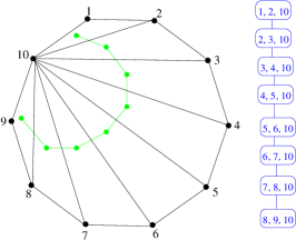
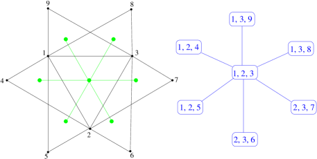
(a)	(b)

Figure 3: Graph representing (a) chain junction tree, (b) star junction tree, with an embedded junction tree in green and its junction tree representation in blue.

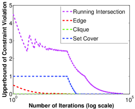
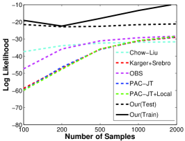
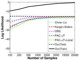
(a)	(b)	(c)

Figure 4: Left: (a) Upper bound of constraint violations for d=2 and a chain junction tree. Right: Log likelihood of the structures learnt using various algorithms on (b) TRAFFIC and (c) ALARM datasets with $k=3$ except Chow-Liu $(k=1)$.

Table 1: Performance on chain junction trees. See text for details.

d	$\Delta$Dual	$\Delta$Dualr	$\Delta$Primal	$\Delta$Primalr	$\Delta$Greedy
1	-0.7$\pm$0.1	-32.7$\pm$16.4	0.2$\pm$0.1	0.4$\pm$0.1	0.2$\pm$0.1
2	-0.4$\pm$0.1	-23.4$\pm$9.6	0	0.3$\pm$0.2	0.5$\pm$0.2
4	-1.1$\pm$0.1	-31.2$\pm$9.7	0	0.3$\pm$0.1	1.9$\pm$0.3
8	-0.6$\pm$0.1	-23.9$\pm$9.8	0	0.2$\pm$0.1	7.9$\pm$0.3
16	-1.9$\pm$0.2	- 3.4$\pm$2.7	0	0	25.6$\pm$1.2
32	-3.9$\pm$0.5	- 3.2$\pm$0.3	0	0	57.3$\pm$1.5

Table 2: Performance on star junction trees. See text for details.

d	$\Delta$Dual	$\Delta$Dualr	$\Delta$Primal	$\Delta$Primalr	$\Delta$Greedy
1	-0.8$\pm$0.1	-31.4$\pm$13.4	0.2$\pm$0.1	0.5$\pm$0.1	0.9$\pm$0.1
2	-0.5$\pm$0.2	-26.6$\pm$13.3	0	0.4$\pm$0.1	0.4$\pm$0.3
4	-0.3$\pm$0.0	-16.6$\pm$4.1	0	0.2$\pm$0.1	1.7$\pm$0.2
8	-0.4$\pm$0.0	-16.0$\pm$9.6	0	0	6.9$\pm$0.3
16	-1.2$\pm$0.5	-3.1$\pm$0.3	0	0	26.3$\pm$1.5
32	-6.8$\pm$0.4	-8.5$\pm$1.2	0	0	58.3$\pm$1.9

Performance Comparison.

We compare the quality of the graph structures learned by the proposed algorithm with the ones produced by Ordering Based Search (OBS) [31], the combinatorial optimization algorithm proposed by Karger and Srebro (Karger+Srebro) [15], the Chow-Liu trees (Chow-Liu) [7] and different variations of PAC-learning based algorithms (PAC-JT, PAC-JT+local) [6]. We use a real-world dataset, TRAFFIC [18] and an artificial dataset, ALARM [2] to compare the performances of these algorithms.

This ALARM dataset was sampled from a known Bayesian network [2] of 37 nodes, which has a treewidth equal to 4. We learn an approximate decomposable graph of treewidth 3. The TRAFFIC dataset is the traffic flow information every 5 minutes for a month at 8000 locations in California [18]. The traffic flow information is collected at 32 locations in San Francisco Bay area and the values are discretized into 4 bins. We learn an approximate decomposable graph of treewidth 3 using our approach. Empirical entropies are computed from the generated samples of each data set and we infer the underlying structure from them using our algorithm. Figure 4(b) and Figure 4(c) show the log-likelihoods of structures learnt using various algorithms on Traffic and Alarm datasets respectively. Note that the performance is better with higher values as we compare log-likelihoods. These figures illustrate the gains of the convex approach over the earlier non-convex approaches.

6 Conclusion and Future Work

In this paper, we have provided a convex relaxation to the problem of finding the maximum likelihood decomposable graph with bounded treewidth, with a polynomial-time optimization algorithm, which empirically outperforms previously proposed algorithms. We are currently exploring two avenues for improvements: (a) design sufficient conditions for tightness of our relaxation, following the recent literature on relaxation of variable selection problems [5], and (b) use heuristics to speed-up the algorithms to allow application to larger graphs.

Acknowledgements

We acknowledge support from the European Research Council grant SIERRA (project 239993), and would like to thank Anton Chechetka, Carlos Guestrin, Nathan Srebro and Percy Liang for sharing code and datasets. We would also like to thank other members of the SIERRA and WILLOW project-teams for helpful discussions.

References

- [1] F. Bach and M. Jordan. Thin junction trees. In Adv. NIPS, 2002.
- [2] I. A. Beinlich, H. J. Suermondt, R. M. Chavez, and G. F. Cooper. The ALARM Monitoring System: A Case Study with Two Probabilistic Inference Techniques for Belief Networks. In Proc. of Euro. Conf. on AI in Medicine, 1989.
- [3] D. P. Bertsekas. Nonlinear Programming. Athena Scientific, 1999.
- [4] C. Bishop et al. Pattern recognition and machine learning. springer New York, 2006.
- [5] E. Candès and T. Tao. Decoding by linear programming. IEEE Trans. Information Theory, 51(12):4203–4215, 2005.
- [6] A. Chechetka and C. Guestrin. Efficient principled learning of thin junction trees. In Adv. NIPS, 2007.
- [7] C. I. Chow and C. N. Liu. Approximating discrete probability distributions with dependence trees. IEEE Trans. Inf. Theory, 14, 1968.
- [8] T. M. Cover and J. A. Thomas. Elements of information theory. John Wiley & Sons, 2006.
- [9] A. Deshpande, M. Garofalakis, and M. Jordan. Efficient stepwise selection in decomposable models. In Proc. UAI, 2001.
- [10] A. Frank, T. Király, and M. Kriesell. On decomposing a hypergraph into k connected sub-hypergraphs. Discrete Applied Mathematics, 131(2):373–383, 2003.
- [11] N. Friedman and D. Koller. Being Bayesian about network structure. a bayesian approach to structure discovery in bayesian networks. Machine learning, 50(1):95–125, 2003.
- [12] T. Fukunaga. Computing minimum multiway cuts in hypergraphs from hypertree packings. Integer Prog. Comb. Optimization, pages 15–28, 2010.
- [13] V. Gogate, W. Webb, and P. Domingos. Learning efficient Markov networks. In Adv. NIPS, 2010.
- [14] M. C. Golumbic. Algorithmic Graph Theory and Perfect Graphs. North Holland, 2004.
- [15] D. Karger and N. Srebro. Learning Markov networks: maximum bounded tree-width graphs. In Proc. ACM-SIAM symposium on Discrete algorithms, 2001.
- [16] D. Koller and N. Friedman. Probabilistic graphical models: principles and techniques. MIT press, 2009.
- [17] V. Kolmogorov and T. Schoenemann. Generalized sequential tree-reweighted message passing. ArXiv e-prints, May 2012.
- [18] A. Krause and C. Guestrin. Near-optimal nonmyopic value of information in graphical models. In Proc. UAI, 2005.
- [19] S. L. Lauritzen. Graphical Models. Oxford University Press, Oxford, 1996.
- [20] M. Lorea. Hypergraphes et matroides. Cahiers Centre Etud. Rech. Oper, 17:289–291, 1975.
- [21] F. Malvestuto. Approximating discrete probability distributions with decomposable models. IEEE Trans. Systems, Man, Cybernetics, 21(5), 1991.
- [22] M. Narasimhan and J. Bilmes. PAC-learning bounded tree-width graphical models. In Proc. UAI, 2004.
- [23] A. Nedić and A. Ozdaglar. Approximate primal solutions and rate analysis for dual subgradient methods. SIAM J. Opt., 19(4), Feb. 2009.
- [24] L. Saul and M. Jordan. Exploiting tractable substructures in intractable networks. In Adv. NIPS, 1995.
- [25] A. Schrijver. Combinatorial optimization: Polyhedra and efficiency. Springer, 2004.
- [26] D. Shahaf, A. Chechetka, and C. Guestrin. Learning thin junction trees via graph cuts. In Artificial Intelligence and Statistics (AISTATS), 2009.
- [27] P. Spirtes, C. Glymour, and R. Scheines. Causation, prediction, and search, volume 81. MIT press, 2001.
- [28] N. Srebro. Maximum likelihood bounded tree-width Markov networks. In Proc. UAI, 2002.
- [29] T. Szántai and E. Kovács. Discovering a junction tree behind a Markov network by a greedy algorithm. ArXiv e-prints, Apr. 2011.
- [30] T. Szántai and E. Kovács. Hypergraphs as a mean of discovering the dependence structure of a discrete multivariate probability distribution. Annals OR, 193(1), 2012.
- [31] M. Teyssier and D. Koller. Ordering-based search: A simple and effective algorithm for learning bayesian networks. In Proc. UAI, 2005.
- [32] M. Wainwright and M. Jordan. Graphical models, exponential families, and variational inference. Found. and Trends in Mach. Learn., 1(1-2), 2008.