PoS(Lattice 2012)116
ADP-12-50/T817
DESY 12-229
Edinburgh 2012/23
Liverpool LTH 967

The effects of flavour symmetry breaking on hadron matrix elements

Abstract:

By considering a flavour expansion about the $SU(3)$-flavour symmetric point, we investigate how flavour-blindness constrains octet baryon matrix elements after $SU(3)$ is broken by the mass difference between the strange and light quarks. We find the expansions to be highly constrained along a mass trajectory where the singlet quark mass is held constant, which proves beneficial for extrapolations of 2+1 flavour lattice data to the physical point. We investigate these effects numerically via a lattice calculation of the flavour-conserving and flavour-changing matrix elements of the vector and axial operators between octet baryon states.

1 Introduction

Understanding the pattern of flavour symmetry breaking and mixing, and the origin of CP violation, remains one of the outstanding problems in particle physics. In [1, 2] we have outlined a program to systematically investigate the pattern of flavour symmetry breaking. The program has been successfully applied to meson and baryon masses involving up, down and strange quarks. In these talks we will extend the investigations to include matrix elements.

The QCD interaction is flavour-blind. Neglecting electromagnetic and weak interactions, the only difference between flavours comes from the mass matrix. We investigate how flavour-blindness constrains matrix elements after flavour $SU(3)$ is broken by the mass difference between the strange and light quarks, to help us extrapolate $2+1$ flavour lattice data to the physical point.

We have our best theoretical understanding when all 3 quark flavours have the same masses (because we can use the full power of flavour $SU(3)$); nature presents us with just one instance of the theory, with $m_{s}/m_{l}\approx 25.$ On the lattice we can choose our quark masses, so we can investigate fictional universes where $m_{s}/m_{l}\neq 25$, and so gain a clearer understanding of flavour symmetry breaking.

We have previously used a symmetry analysis, similar in spirit to that used by Gell-Mann and Okubo [3, 4] in the earliest days of the quark picture, to find formulae for the quark mass dependence of hadron masses [1, 2]. We now extend this analysis to hadron matrix elements. In the first part of these proceedings we discuss the group theory, in the second part we compare our expectations with lattice data. We shall then discuss briefly the further steps needed to compute form factors relevant to the determination of the CKM matrix element $|V_{us}|$.

In this work we concentrate on the $2+1$ case, in which symmetry breaking is due to mass differences between the strange and light quarks; but our methods are also applicable to isospin breaking effects coming from a non-zero $m_{d}-m_{u}$, e.g. [5].

2 $SU(3)$ breaking

How severely does the strange quark mass break $SU(3)$ symmetry? In this approach it is not the strange-light ratio, $m_{s}/m_{l}\sim 25$, which matters. A more natural way to judge the severity of symmetry breaking is to compare $(m_{s}-m_{l})$ with a typical hadronic mass. Since $(m_{s}-m_{l})\ll M_{B}$ we can hope for an expansion with very good convergence.

We can see how well this works in practice by looking, for example, at the physical masses of the decuplet baryons. We can construct mass combinations which first appear at different orders of the symmetry breaking, starting with quantities that would be non-zero even with perfect $SU(3)$, and working up to quantities which first appear at the third order in the symmetry breaking parameter

$$4M_{\Delta}+3M_{\Sigma^{*}}+2M_{\Xi^{*}}+M_{\Omega} = +13.82{\rm\ GeV}\qquad\quad\ {\rm singlet}\quad\propto(m_{s}-m_{l})^{0}$$

$$-2M_{\Delta}\qquad\ \quad+M_{\Xi^{*}}+M_{\Omega} = +0.742{\rm\ GeV}\qquad\quad\ {\rm octet}\quad\,\,\,\,\,\,\propto(m_{s}-m_{l})^{1}$$

$$4M_{\Delta}-5M_{\Sigma^{*}}-2M_{\Xi^{*}}+3M_{\Omega} = -0.044{\rm\ GeV}\qquad\quad\mbox{27-plet}\quad\propto(m_{s}-m_{l})^{2}$$

$$-M_{\Delta}+3M_{\Sigma^{*}}-3M_{\Xi^{*}}+M_{\Omega} = -0.006{\rm\ GeV}\qquad\quad\mbox{64-plet}\quad\propto(m_{s}-m_{l})^{3}\,,$$ (1)

where we have used the isospin-averaged experimental masses for each decuplet baryon. Clearly we see a strong hierarchy in values. Each additional factor of $(m_{s}-m_{l})$ reduces the value by about an order of magnitude, the final $O((m_{s}-m_{l})^{3})$ quantity is about $2000$ times smaller than the leading quantity. An expansion that yields a factor of $10$ for each order is very good compared with most approaches available for QCD.

To investigate flavour symmetry breaking systematically, we need to vary the amount of symmetry beaking we have, while keeping all the flavour singlet terms in the action constant. We therefore follow a strategy in which the average quark mass $\overline{m}\equiv(m_{u}+m_{d}+m_{s})/3$ is kept constant, while the mass splitting is increased. Our notation for the quark masses and their splittings is

$$\overline{m} \equiv \frac{1}{3}(m_{u}+m_{d}+m_{s})\quad{\rm fixed}$$

$$\delta{m}_{u} \equiv m_{u}-\overline{m}$$

$$\delta{m}_{d} \equiv m_{d}-\overline{m}$$ (2)

$$\delta{m}_{s} \equiv m_{s}-\overline{m}$$

$$m_{l} \equiv \frac{1}{2}(m_{u}+m_{d})$$

$$\delta{m}_{l} \equiv m_{l}-\overline{m}\,.$$

From these definitions we have the identity $\delta{m}_{u}+\delta{m}_{d}+\delta{m}_{s}=0$. In this notation the quark mass matrix is

$${\cal M} = \pmatrix{m_{u}&0&0\cr 0&m_{d}&0\cr 0&0&m_{s}}$$ (3)

$$= \overline{m}\pmatrix{1&0&0\cr 0&1&0\cr 0&0&1}+{\textstyle\frac{1}{2}}(\delta{m}_{u}-\delta{m}_{d})\pmatrix{1&0&0\cr 0&-1&0\cr 0&0&0}+{\textstyle\frac{1}{2}}\delta{m}_{s}\pmatrix{-1&0&0\cr 0&-1&0\cr 0&0&2}\,.$$

${\cal M}$ has a flavour singlet part (proportional to $I$) and a flavour octet part, proportional to $\lambda_{3}$, $\lambda_{8}$. It is important to note that there are no terms in the QCD Lagrangian which are in representations higher than the octet. The only way to give a value to a quantity in a higher $SU(3)$ representation is to have multiple powers of the flavour-breaking term, i.e. multiple powers of $\delta m_{q}$.

Therefore we adopt the following strategy. We classify physical quantities by their representation of $SU(3)$ and its sub-group $SU(2)$, and classify quark mass polynomials in the same way. The Taylor expansion of a quantity of known symmetry can only involve polynomials of the matching symmetry. This strongly constrains the Taylor expansion of physical quantities about a symmetric point with all three quark masses equal.

In this work we are investigating non-singlet matrix elements (e.g. vector and axial-vector currents for weak decays) acting between octet baryons. This octet is illustrated in Fig. 1.

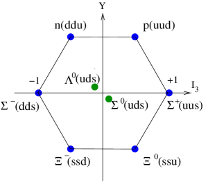
Figure 1: The (lowest) octet baryon states.

The matrix elements have the form $\langle B^{i}|O^{j}|B^{k}\rangle$ with $i,j,k\in\{1,\cdots,8\}$ because the hadrons and operators are both in flavour octets. Our choice of indices is set out in Table 1. We use the corresponding meson name to refer

Index	Baryon ($B$)	Meson ($M$)	Operator ($O$)
1	$n$	$K^{0}$	$\bar{d}\gamma s$
2	$p$	$K^{+}$	$\bar{u}\gamma s$
3	$\Sigma^{-}$	$\pi^{-}$	$\bar{d}\gamma u$
4	$\Sigma^{0}$	$\pi^{0}$	$\frac{1}{\sqrt{2}}\left(\bar{u}\gamma u-\bar{d}\gamma d\right)$
5	$\Lambda^{0}$	$\eta$	$\frac{1}{\sqrt{6}}\left(\bar{u}\gamma u+\bar{d}\gamma d-2\bar{s}\gamma s\right)$
6	$\Sigma^{+}$	$\pi^{+}$	$\bar{u}\gamma d$
7	$\Xi^{-}$	$K^{-}$	$\bar{s}\gamma u$
8	$\Xi^{0}$	$\bar{K}^{0}$	$\bar{s}\gamma d$

Table 1: Our numbering of the octet states, used internally. Whenever possible, final results will be presented in ways that are independent of the index choice. We use the convention that operator number $i$ has the same effect as absorbing a meson with the index $i$.

to the flavour of bilinear quark operators, for example

$$\langle p|\pi^{0}|p\rangle\equiv\langle p|\frac{1}{\sqrt{2}}(\overline{u}\gamma u-\overline{d}\gamma d)|p\rangle\equiv\langle B^{2}|O^{4}|B^{2}\rangle\,,$$ (4)

where $\gamma$ is a generic gamma matrix. Since we need three indices, $i$, $j$, $k$, to specify a matrix element, we now need to classify $8\times 8\times 8$ tensors under $SU(3)$, in just the same way as we needed to give the classification of $8\times 8$ and $10\times 10$ matrices for baryon masses.

To find the allowed mass-dependence of octet matrix elements of octet hadrons we need the $SU(3)$ decomposition of $8\otimes 8\otimes 8$. Using the intermediate result

$$8\otimes 8=1\oplus 8\oplus 8\oplus 10\oplus{\overline{10}}\oplus 27\,,$$ (5)

we find

$$\!\!8\otimes 8\otimes 8\!\! = \!\!1\oplus 1\oplus 8\oplus 8\oplus 8\oplus 8\oplus 8\oplus 8\oplus 8\oplus 8$$ (6)

$$\!\!\oplus 27\oplus 27\oplus 27\oplus 27\oplus 27\oplus 27\oplus{64}$$

$$\!\!\oplus 10\oplus 10\oplus 10\oplus 10\oplus{\overline{10}}\oplus{\overline{10}}\oplus{\overline{10}}\oplus{\overline{10}}$$

$$\!\!\oplus 35\oplus 35\oplus{\overline{35}}\oplus{\overline{35}}\,.$$

The allowed quark mass Taylor expansion for a hadronic matrix element must follow the schematic pattern

$$\langle H^{i}|O^{j}|H^{k}\rangle = \sum(\mbox{singlet mass polynomial})\times(\mbox{singlet tensor})^{ijk}$$

$$+\sum(\mbox{octet mass polynomial})\times(\mbox{octet tensor})^{ijk}$$

$$+\sum(\mbox{27-plet mass polynomial})\times(\mbox{27-plet tensor})^{ijk}$$

$$+\sum(\mbox{64-plet mass polynomial})\times(\mbox{64-plet tensor})^{ijk}$$

$$+\ \cdots\,.$$

The tensors in this equation are three-dimensional arrays of integers and square-roots of integers, objects somewhat analogous to three-dimensional Gell-Mann matrices.

Mass polynomials with the symmetry $10$, $\overline{10}$, $35$, $\overline{35}$ all have factors of $(m_{u}-m_{d})$. So they only appear if we consider the $1+1+1$ case of symmetry breaking. At present we are only considering the $2+1$ case, $m_{u}=m_{d}\neq m_{s}$ so we can neglect the $10$, $\overline{10}$, $35$, $\overline{35}$ representations.

We found just two singlet tensors in the expansion of $8\otimes 8\otimes 8$, so at the symmetric point there are only two independent coefficients (usually called $F,D$ or $f,d$) needed to completely specify all the matrix elements between the members of the octet. These give the classic $SU(3)$ inter-relations between octet amplitudes. These are generally found to work rather well. We should however be able to do better by also including higher terms in the mass expansion.

There are $8$ octets in the expansion of $8\otimes 8\otimes 8$, so if we work to first order $\delta m_{q}$, the $SU(3)$ flavour violation, we have $8$ new coefficients. There are still many fewer coefficients than there are amplitudes, so there are numerous constraints and cross-relations between amplitudes. The singlet and octet tensors are given explicitly in Table 2.

		1		8
$I$	$A_{\overline{B}^{\prime}MB}$	$f$	$d$	$r_{1}$	$r_{2}$	$r_{3}$	$r_{4}$	$r_{5}$	$s_{1}$	$s_{2}$	$s_{3}$
$0$	${\overline{N}\eta N}$	$\sqrt{3}$	$-1$	1	0	0	0	0	0	$-1$	0
$0$	${\overline{\Sigma}\eta\Sigma}$	0	2	1	0	$2\sqrt{3}$	0	0	0	0	0
$0$	${\overline{\Lambda}\eta\Lambda}$	0	$-2$	1	2	0	0	0	0	0	0
$0$	${\overline{\Xi}\eta\Xi}$	$-\sqrt{3}$	$-1$	1	0	0	0	0	0	1	0
$1$	${\overline{N}\pi N}$	1	$\sqrt{3}$	0	0	$-2$	0	0	2	0	0
$1$	${\overline{\Sigma}\pi\Sigma}$	2	0	0	0	0	0	0	$-2$	$\sqrt{3}$	0
$1$	${\overline{\Xi}\pi\Xi}$	1	$-\sqrt{3}$	0	0	$2$	0	0	2	0	0
$1$	${\overline{\Sigma}\pi\Lambda}$	0	2	0	1	$-\sqrt{3}$	$i$	0	0	0	0
$1$	${\overline{\Lambda}\pi\Sigma}$	0	2	0	1	$-\sqrt{3}$	$-i$	0	0	0	0
$\frac{1}{2}$	${\overline{N}K\Sigma}$	$-\sqrt{2}$	$\sqrt{6}$	0	0	$\sqrt{2}$	0	$i\sqrt{2}$	$\sqrt{2}$	0	$i\sqrt{6}$
$\frac{1}{2}$	${\overline{N}K\Lambda}$	$-\sqrt{3}$	$-1$	0	1	0	$i$	$i\sqrt{3}$	$-\sqrt{3}$	1	$-i$
$\frac{1}{2}$	${\overline{\Lambda}K\Xi}$	$\sqrt{3}$	$-1$	0	1	0	$-i$	$-i\sqrt{3}$	$\sqrt{3}$	$-1$	$-i$
$\frac{1}{2}$	${\overline{\Sigma}K\Xi}$	$\sqrt{2}$	$\sqrt{6}$	0	0	$\sqrt{2}$	0	$-i\sqrt{2}$	$-\sqrt{2}$	0	$i\sqrt{6}$
$\frac{1}{2}$	${\overline{\Sigma}\overline{K}N}$	$-\sqrt{2}$	$\sqrt{6}$	0	0	$\sqrt{2}$	0	$-i\sqrt{2}$	$\sqrt{2}$	0	$-i\sqrt{6}$
$\frac{1}{2}$	${\overline{\Lambda}\overline{K}N}$	$-\sqrt{3}$	$-1$	0	1	0	$-i$	$-i\sqrt{3}$	$-\sqrt{3}$	1	$i$
$\frac{1}{2}$	${\overline{\Xi}\overline{K}\Lambda}$	$\sqrt{3}$	$-1$	0	1	0	$i$	$i\sqrt{3}$	$\sqrt{3}$	$-1$	$i$
$\frac{1}{2}$	${\overline{\Xi}\overline{K}\Sigma}$	$\sqrt{2}$	$\sqrt{6}$	0	0	$\sqrt{2}$	0	$i\sqrt{2}$	$-\sqrt{2}$	0	$-i\sqrt{6}$

Table 2: Coefficients in the mass Taylor expansion of operator amplitudes: $SU(3)$ singlet and octet. These coefficients are sufficient for the linear expansion of hadronic amplitudes.

This table gives the amplitudes for the baryons $p$, $\Lambda^{0}$, $\Sigma^{+}$, $\Xi^{0}$; the amplitudes for the other baryons can be deduced from isospin symmetry (which we are, for now, treating as unbroken). We have used the notation for the matrix element transition $B\to B^{\prime}$ of

$$A_{\overline{B}^{\prime}MB}=\langle B^{\prime}|M|B\rangle\,,$$ (8)

where $M$ is the appropriate operator from Table 1. We illustrate how this table works by reading off the mass expansion for the first two amplitudes

$$\langle p|\eta|p\rangle=A_{\overline{N}\eta N} = \sqrt{3}f-d+(r_{1}-s_{2})\delta{m}_{l}$$

$$\langle\Sigma^{+}|\eta|\Sigma^{+}\rangle=A_{\overline{\Sigma}\eta\Sigma} = 2d+(r_{1}+2\sqrt{3}r_{3})\delta{m}_{l}$$ (9)

$$\vdots$$

3 ‘Fan’ Plots

In the case of hadron masses we found that ‘fan’ plots were a useful way to display our results, see e.g. Fig. 20 of [2]. We plotted the masses of the hadrons in a multiplet against $\delta{m}_{l}=m_{l}-\overline{m}$. When $\delta{m}_{l}=0$ (the $SU(3)$ symmetric point) all masses are equal, as we increase the symmetry breaking the masses fan out, about an ‘average’ mass which is almost constant.

We can display matrix elements in a similar way. Some matrix elements, however, will be protected from first order flavour symmetry breaking effects. The Ademollo–Gatto theorem, [6], for example, states that certain form factors for vector currents will not display $\delta{m}_{l}$ effects.

3.1 The $f$-fan

Using Table 2 we can construct five quantities $F_{i}$, which all have the same value ($2f$) at the symmetric point, but which can differ once $SU(3)$ is broken.

$$F_{1}\equiv\frac{1}{\sqrt{3}}(A_{\bar{N}\eta N}-A_{\bar{\Xi}\eta\Xi}) = 2f-\frac{2}{\sqrt{3}}s_{2}\delta{m}_{l}$$

$$F_{2}\equiv(A_{\bar{N}\pi N}+A_{\bar{\Xi}\pi\Xi}) = 2f+4s_{1}\delta{m}_{l}$$

$$F_{3}\equiv A_{\bar{\Sigma}\pi\Sigma} = 2f+(-2s_{1}+\sqrt{3}s_{2})\delta{m}_{l}$$ (10)

$$F_{4}\equiv\frac{1}{\sqrt{2}}\Re(A_{\bar{\Sigma}K\Xi}-A_{\bar{N}K\Sigma}) = 2f-2s_{1}\delta{m}_{l}$$

$$F_{5}\equiv\frac{1}{\sqrt{3}}\Re(A_{\bar{\Lambda}K\Xi}-A_{\bar{N}K\Lambda}) = 2f+\frac{2}{\sqrt{3}}(\sqrt{3}s_{1}-s_{2})\delta{m}_{l}\,.$$

Plotting these quantities gives a ‘fan’ plot with $5$ lines, but only $2$ slope parameters ($s_{1}$, $s_{2}$), so the splittings between these observables are highly constrained.

A useful ‘average F’ can be constructed from the diagonal amplitudes

$$X_{F}=\frac{1}{6}(3F_{1}+F_{2}+2F_{3})=2f+O(\delta{m}_{l}^{2})\,.$$ (11)

We expect that a ‘fan’ plot of $\tilde{F}_{i}\equiv F_{i}/X_{F}$ might be less noisy than a plot of $F_{i}$ alone. (Using $\tilde{F}_{i}$ rather than $F_{i}$ would also remove renormalisation constants, see eq. (27).) In general we shall denote quantities with a tilde that have been normalised with an appropriate $X$.

3.2 The $d$-fan

Similarly, we can construct seven quantities $D_{i}$, which all have the same value ($2d$) at the symmetric point, but which can differ once $SU(3)$ is broken.

$$D_{1}\equiv-(A_{\bar{N}\eta N}+A_{\bar{\Xi}\eta\Xi}) = 2d-2r_{1}\delta{m}_{l}$$

$$D_{2}\equiv A_{\bar{\Sigma}\eta\Sigma} = 2d+(r_{1}+2\sqrt{3}r_{3})\delta{m}_{l}$$

$$D_{3}\equiv{}-A_{\bar{\Lambda}\eta\Lambda} = 2d-(r_{1}+2r_{2})\delta{m}_{l}$$

$$D_{4}\equiv\frac{1}{\sqrt{3}}(A_{\bar{N}\pi N}-A_{\bar{\Xi}\pi\Xi}) = 2d-\frac{4}{\sqrt{3}}r_{3}\delta{m}_{l}$$ (12)

$$D_{5}\equiv\Re A_{\bar{\Sigma}\pi\Lambda} = 2d+(r_{2}-\sqrt{3}r_{3})\delta{m}_{l}$$

$$D_{6}\equiv\frac{1}{\sqrt{6}}\Re(A_{\bar{N}K\Sigma}+A_{\bar{\Sigma}K\Xi}) = 2d+\frac{2}{\sqrt{3}}r_{3}\delta{m}_{l}$$

$$D_{7}\equiv-\Re(A_{\bar{N}K\Lambda}+A_{\bar{\Lambda}K\Xi}) = 2d-2r_{2}\delta{m}_{l}\,.$$

Plotting these quantities gives a ‘fan’ plot with $7$ lines, but only $3$ slope parameters ($r_{1},r_{2}$ and $r_{3}$), so once again the splittings between these observables are highly constrained. Again it is possible to construct an ‘average D’ similar to $X_{F}$

$$X_{D}=\frac{1}{4}(D_{1}+2D_{2}+D_{4})=2d+O(\delta{m}_{l}^{2})\,,$$ (13)

in order to produce a less noisy ‘fan’ plot.

4 Lattice Calculations

In order to extract the matrix elements for some operator $O$, it is necessary to take an appropriate ratio of three and two-point correlation functions, [7, 8]

$${\cal R}=\frac{C_{3}^{B\rightarrow B^{\prime}}(t,\tau;p,p^{\prime})}{C_{2}^{B^{\prime}}(t,p^{\prime})}\sqrt{\frac{C_{2}^{B^{\prime}}(t,p^{\prime})C_{2}^{B^{\prime}}(\tau,p^{\prime})C_{2}^{B}(t-\tau,p)}{C_{2}^{B}(t,p)C_{2}^{B}(\tau,p)C_{2}^{B^{\prime}}(t-\tau,p^{\prime})}}\,,$$ (14)

where

$$C_{3}^{B\to B^{\prime}}(t,\tau;p,p^{\prime}) = \mbox{tr}_{D}\,\Gamma\langle{\cal B}_{B^{\prime}}(t;\vec{p}^{\prime})O(\tau;\vec{q})\overline{\cal B}_{B}(0;\vec{p})\rangle$$

$$C_{2}^{B}(t,p) = \mbox{tr}_{D}\,\Gamma_{unpol}\langle{\cal B}_{B}(t;\vec{p})\overline{\cal B}_{B}(0;\vec{p})\rangle\,.$$ (15)

This is designed so that any smearing for the source (at time $0$) and sink operators (at time $t$) is cancelled in the ratios, [9]; of course smearing improves the overlap with the lowest lying state. The baryon operators used are as follows

$${\cal B}_{N\,\alpha}(t;\vec{p}) = \sum_{\vec{x}}e^{-i\vec{p}\cdot\vec{x}}\epsilon_{ijk}u_{i\alpha}(\vec{x},t)(u^{T_{D}}_{j}(\vec{x},t)C\gamma_{5}d_{k}(\vec{x},t))$$

$${\cal B}_{\Sigma\,\alpha}(t;\vec{p}) = \sum_{\vec{x}}e^{-i\vec{p}\cdot\vec{x}}\epsilon_{ijk}u_{i\alpha}(\vec{x},t)(u^{T_{D}}_{j}(\vec{x},t)C\gamma_{5}s_{k}(\vec{x},t))$$

$${\cal B}_{\Lambda\,\alpha}(t;\vec{p}) = \sum_{\vec{x}}e^{-i\vec{p}\cdot\vec{x}}\epsilon_{ijk}s_{i\alpha}(\vec{x},t)(u^{T_{D}}_{j}(\vec{x},t)C\gamma_{5}d_{k}(\vec{x},t))$$

$${\cal B}_{\Xi\,\alpha}(t;\vec{p}) = \sum_{\vec{x}}e^{-i\vec{p}\cdot\vec{x}}\epsilon_{ijk}s_{i\alpha}(\vec{x},t)(s^{T_{D}}_{j}(\vec{x},t)C\gamma_{5}u_{k}(\vec{x},t))\,,$$ (16)

where $C$ is the charge conjugation matrix and $i,j,k$ are colour indices and $\alpha$ is a Dirac index. The $u$ and $d$ quarks are treated distinctly, but with degenerate mass. The transferred momentum from the initial, $B$, to final, $B^{\prime}$ state is given by

$$q=p-p^{\prime}=\left(i(E_{B}(\vec{p})-E_{B^{\prime}}(\vec{p}^{\prime})),\vec{p}-\vec{p}^{\prime}\right)\,.$$ (17)

In this study we shall restrict ourselves to zero $3$-momentum transfer, i.e. $\vec{p}=\vec{p}^{\prime}=0$ when

$$q^{2}\to q^{2}_{max}=-(M_{B}-M_{B^{\prime}})^{2}\,,$$ (18)

such that postive $q^{2}$ is spacelike while negative $q^{2}$ is a timelike quantity. The energy of the initial and final states are now simply the rest masses $M_{B}$ and $M_{B^{\prime}}$ respectively. We shall also consider the time-like component of the vector and axial-vector currents as described in Table 1 by taking $M=\pi^{0}$ (or $\pi^{+}$) and $\gamma=\gamma_{4}$ or $M=K^{+}$ and $\gamma=\gamma_{3}\gamma_{5}$ respectively. For example we can set $O$ to be

$$\left.\begin{array}[]{ccc}V_{4}&=&\overline{u}\gamma_{4}d\\ A_{3}&=&\overline{u}\gamma_{3}\gamma_{5}d\\ \end{array}\right\}\,\,\mbox{for $\Delta S=0$ decays}\,,\qquad\left.\begin{array}[]{ccc}V_{4}&=&\overline{u}\gamma_{4}s\\ A_{3}&=&\overline{u}\gamma_{3}\gamma_{5}s\\ \end{array}\right\}\,\,\mbox{for $\Delta S=1$ decays}\,.$$ (23)

Even though in this case $\vec{p}=\vec{p}^{\prime}=0$, in general there is still a $4$-momentum transfer and we usually have a non-forward matrix element. Thus we have

$${\cal R}\rightarrow A_{\overline{B}^{\prime}MB}(q^{2}_{max})\,,\quad\mbox{as}\quad t\,,\,t-\tau\to\infty\,,$$ (24)

depending on whether we are considering the vector $O=V_{4}$, $\Gamma=\Gamma_{unpol}$ or axial-vector $O=A_{3}$, $\Gamma=\Gamma_{pol}$ three-point function.

The computed matrix elements are bare (or lattice) quantities and must be renormalised,

$$V_{4}^{\mbox{\tiny$R$}}=Z_{V}V_{4}\,,\qquad A_{3}^{\mbox{\tiny$R$}}=Z_{A}A_{3}\,,$$ (25)

where we have denoted the renormalised matrix elements with a superscript R. If $A^{\mbox{\tiny$R$}}_{\overline{B}^{\prime}M^{V}B}$ is known then the renormalisation constant can simply be determined from

$$Z_{V}={A^{\mbox{\tiny$R$}}_{\overline{B}^{\prime}M^{V}B}\over A_{\overline{B}^{\prime}M^{V}B}}\,,\qquad Z_{A}={A^{\mbox{\tiny$R$}}_{\overline{B}^{\prime}M^{A}B}\over A_{\overline{B}^{\prime}M^{A}B}}\,.$$ (26)

Alternatively by considering ratios in the ‘fan’ plots the renormalisation constant cancels, for example

$$\tilde{F}^{A}_{i}={F_{i}^{A}\over X_{F^{A}}}={F_{i}^{A\,\mbox{\tiny$R$}}\over X^{\mbox{\tiny$R$}}_{F^{A}}}=\tilde{F}_{i}^{A\,\mbox{\tiny$R$}}\,,\quad i=1\,\ldots\,,5\,,$$ (27)

and similarly for $\tilde{F}_{i}^{V}$, $\tilde{D}_{i}^{A}$ and $\tilde{D}_{i}^{V}$.

The renormalised vector $f$ and $d$ coefficients are known (i.e. the matrix elements at the $SU(3)$ flavour symmetric point). The vector current, being conserved there, essentially just counts the number of quarks. For example using eq. (9) we have

$$A_{\overline{N}\eta^{V}N}^{\mbox{\tiny$R$}} = {1\over\sqrt{6}}(2+1-0)=\sqrt{3}f_{V}^{\mbox{\tiny$R$}}-d_{V}^{\mbox{\tiny$R$}}\,,$$

$$A_{\overline{\Sigma}\eta^{V}\Sigma}^{\mbox{\tiny$R$}} = {1\over\sqrt{6}}(2+0-2)=2d_{V}^{\mbox{\tiny$R$}}\,,$$ (28)

giving

$$f_{V}^{\mbox{\tiny$R$}}={1\over\sqrt{2}}\,,\qquad\mbox{and}\quad d_{V}^{\mbox{\tiny$R$}}=0\,.$$ (29)

This result can be used to estimate the renormalisation constant. Either eq. (26) can be used at the symmetric point or equivalently if we have measured $X_{F_{V}}$ ($\gamma=\gamma_{4}$) then from eq. (11) we have up to $O(\delta m_{l}^{2})$

$$Z_{V}={X_{F_{V}}^{\mbox{\tiny$R$}}\over X_{F_{V}}}={2f_{V}^{\mbox{\tiny$R$}}\over X_{F_{V}}}={\sqrt{2}\over X_{F_{V}}}\,,$$ (30)

For the axial current we can connect our conventions with others in the literature, e.g. [12, 13], via

$$f_{A}^{\mbox{\tiny$R$}}={1\over\sqrt{2}}F_{A}\,,\qquad\mbox{and}\quad d_{A}^{\mbox{\tiny$R$}}={1\over\sqrt{6}}D_{A}\,,$$ (31)

at the symmetric point. Similarly to $Z_{V}$ for $Z_{A}$ again either eq. (26) can be used, for example for neutron $\beta$-decay

$$A_{\overline{N}KN}={1\over\sqrt{2}}g_{A}^{\mbox{\tiny$R$}}\,,$$ (32)

where $g_{A}^{\mbox{\tiny$R$}}$ the axial-vector coupling in $\beta$-decay at the physical point. Equivalently from measuring $X_{F_{A}}$ and $X_{D_{A}}$ yields

$$Z_{A}={X_{F_{A}}^{\mbox{\tiny$R$}}\over X_{F_{A}}}={2f_{A}^{\mbox{\tiny$R$}}\over X_{F_{A}}}\,,\qquad\mbox{or}\quad Z_{A}={X_{D_{A}}^{\mbox{\tiny$R$}}\over X_{D_{A}}}={2d_{A}^{\mbox{\tiny$R$}}\over X_{D_{A}}}\,,$$ (33)

(provided that either $X_{F_{A}}^{\mbox{\tiny$R$}}$ or $X_{D_{A}}^{\mbox{\tiny$R$}}$ is known). Alternatively the ratio where $Z_{A}$ cancels is

$${f_{A}\over d_{A}}={X_{F_{A}}\over X_{D_{A}}}\,.$$ (34)

5 Results

In a similar manner to previous simulations [1, 2] our gauge field configurations have been generated with $N_{f}=2+1$ flavours of dynamical fermions, using the tree-level Symanzik improved gluon action and nonperturbatively $O(a)$ improved Wilson fermions, [14]. The quark masses are chosen by first finding the $SU(3)$ flavour symmetric point where flavour singlet quantities take on their physical values and vary the individual quark masses while keeping the singlet quark mass $\overline{m}=(m_{u}+m_{d}+m_{s})/3=(2m_{l}+m_{s})/3$ constant, as described in section 2. Simulations are performed on lattice volumes of $24^{3}\times 48$ at $\beta=5.50$ corresponding to a lattice spacing of $a\approx 0.079$, [2]. Our calculations are performed on $5$ ensembles chosen by methods as also outlined in [2] presently using $\sim 400$–$500$ trajectories for off–diagonal matrix elements $B^{\prime}\not=B$ and $\sim 2000$ trajectories for diagonal matrix elements $B^{\prime}=B$. In Table 3

Ensemble	$\kappa_{l}$	$\kappa_{s}$
1	0.12083	0.12104
2	0.12090	0.12090
3	0.12095	0.12080
4	0.12100	0.12070
5	0.12104	0.12062

Table 3: Ensembles used in calculations here.

we give these $(\kappa_{l},\kappa_{s})$ values used here. Ensemble $2$ corresponds to the symmetric point. Note that for ensemble $1$ we have a universe where the $l$ quarks are heavier than the $s$ quark.

In [5] (see also [2]) the value of the distance away from the symmetric point to the physical point was determined to be $\delta m_{l}^{*}=-0.01102(3)$ in lattice units. (The $*$ denotes the physical point; see eq. (2) for the definition of $\delta m_{l}$.)

5.1 $X_{D}$, $X_{F}$

We first consider $X_{F}$, eq. (11), and $X_{D}$, eq. (13) for the axial-vector case. In Fig. 2

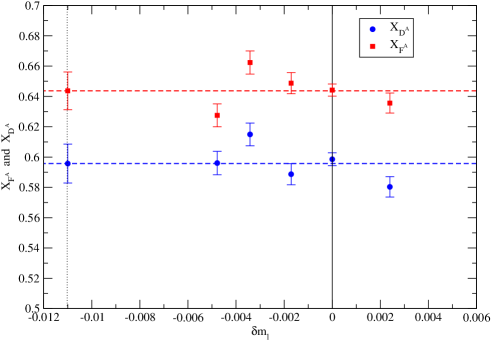
Figure 2: $X_{F^{A}}$ (filled squares), $X_{D^{A}}$ (filled circles) against $\delta m_{l}$ each together with a constant fit.

we plot $X_{F^{A}}$, $X_{D^{A}}$ against $\delta m_{l}$. We expect these quantities to be constant (up to $O(\delta m_{l}^{2})$ terms) and within error bars this is indeed the case. From the values of the constant fits and using eq. (34), we find $f_{A}/d_{A}=1.08(3)$. As it is well known that axial current matrix elements suffer from large finite size effects, we are presently repeating the determination of the matrix elements on larger $32^{3}\times 64$ lattices.

5.2 ‘Fan’ plots

We now turn to a discussion of ‘fan’ plots. As noted previously [2], it is better to consider ratios, which are less noisy. In Fig. 3 we show $\tilde{F}^{A}_{i}=F^{A}_{i}/X_{F_{A}}$

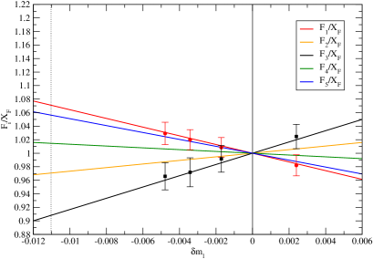
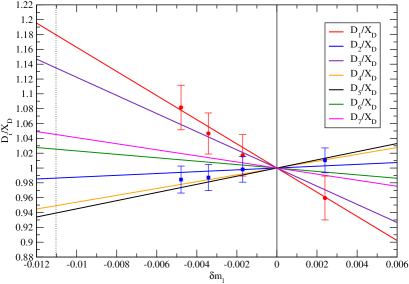
Figure 3: Left panel: $\tilde{F}^{A}_{i}=F^{A}_{i}/X_{F_{A}}$ ($i=1,\,\ldots,\,5$), right panel: $\tilde{D}^{A}_{i}=D^{A}_{i}/X_{D_{A}}$ ($i=1,\,\ldots,\,7$). Shown are just the numerical results for $\tilde{F}^{A}_{1}$ (circles), $\tilde{F}^{A}_{2}$ (squares) and $\tilde{D}^{A}_{1}$ (circles), $\tilde{D}^{A}_{3}$ (squares) against $\delta m_{l}$ together with the (normalised) fits from eqs. (3.2), (3.1).

(left panel) and $\tilde{D}^{A}_{i}=D^{A}_{i}/X_{D_{A}}$ (right panel) together with representive numerical results. (Due to our relatively low number of configurations used in the analysis, error bars overlap if all numerical results are plotted.) Note that because we have normalised the data with $X_{F^{A}}$ or $X_{D^{A}}$ so at the symmetric point the ratios are $1$ exactly.

We make a simultaneous fit to the data to arrive at a determination for the constants $\tilde{s}^{A}_{1}$, $\tilde{s}^{A}_{2}$, $\tilde{s}^{A}_{3}$ and $\tilde{r}^{A}_{1}$, $\tilde{r}^{A}_{2}$, (where $\tilde{s}^{A}_{i}=s^{A}_{i}/2f^{A}$, $\tilde{r}^{A}_{i}=r^{A}_{i}/2d^{A}$) based upon eqs. (3.1), (3.2). Using these parameters it is then possible to reconstruct the equations describing the $SU(3)$ flavour symmetry breaking effects on matrix elements up to $O(\delta m_{l})$. It should be noted that we have yet to perform calculations for certain correlators, though we are progressing in this direction [10]. Those missing include $A_{\bar{\Sigma}K^{A}\Xi}$ which then precludes the use of $F^{A}_{4}$ and $D^{A}_{6}$ in our simultaneous fits. The axial-vector matrix elements clearly have linear terms in $\delta m_{l}$.

For the vector case due to the Ademello–Gatto theorem, [6], the linear terms in $\delta m_{l}$ are absent. So instead of a ‘fan’ plot we show in Fig. 4 a

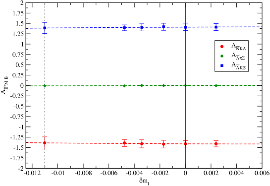
Figure 4: The matrix elements $A_{\overline{N}K^{V}\Lambda}$ (red filled circles), $A_{\overline{\Lambda}\pi^{V}\Sigma}$ (green filled diamonds) and $A_{\overline{\Lambda}K^{V}\Xi}$ (blue filled squares) against $\delta m_{l}$, together with a quadratic fit.

selection of matrix elements $A_{\overline{N}K^{V}\Lambda}$, $A_{\overline{\Lambda}\pi^{V}\Sigma}$, and $A_{\overline{\Lambda}K^{V}\Xi}$. As a check, from Table 2 we see that to leading order $A^{\mbox{\tiny$R$}}_{\overline{\Lambda}\pi^{V}\Sigma}=0+d^{\mbox{\tiny$R$}}_{V}$ i.e. it contains only a $d^{\mbox{\tiny$R$}}_{V}$ term and no $f^{\mbox{\tiny$R$}}_{V}$ term. However $d_{V}^{\mbox{\tiny$R$}}=0$, eq. (29), so we expect to $O(\delta m_{l}^{2})$ that $A_{\overline{\Lambda}\pi^{V}\Sigma}$ vanishes, which is clearly seen in Fig. 4. The other decays are also flat. At the symmetric point (or indeed at other points) we can estimate $Z_{V}$ from eq. (26). As $A^{\mbox{\tiny$R$}}_{\overline{N}K^{V}\Lambda}=-\sqrt{3/2}=-A^{\mbox{\tiny$R$}}_{\overline{\Lambda}K^{V}\Xi}$ then we expect one result in Fig. (4) to be the mirror image of the other. This is the case and choosing $A_{\overline{N}K^{V}\Lambda}$ gives upon using eq. (26), $Z_{V}=0.87(5)$.

6 Octet hyperon semi-leptonic decays

The theory outlined in previous sections is general; most phenomenological calculations are directed towards the semi-leptonic decays $B\to B^{\prime}e\overline{\nu}_{e}$ of various octet hyperons in order to help determine $|V_{us}|$, e.g. [11]. We now briefly indicate how far our programme has reached this goal.

In the Euclidean metric the general form of the matrix element for semi-leptonic transitions $B\to B^{\prime}e\overline{\nu}_{e}$ is

$$\langle B^{\prime}(p^{\prime})|V_{\alpha}(q)+A_{\alpha}(q)|B(p)\rangle=\bar{u}_{B^{\prime}}(p^{\prime})({\cal O}_{\alpha}^{V}(q)+{\cal O}_{\alpha}^{A}(q))u_{B}(p)\,,$$ (35)

where

$${\cal O}_{\alpha}^{V}(q)=\gamma_{\alpha}f_{1}^{\mbox{\tiny$R$}}(q^{2})+\sigma_{\alpha\beta}q_{\beta}\frac{f_{2}^{\mbox{\tiny$R$}}(q^{2})}{M_{B}+M_{B^{\prime}}}+iq_{\alpha}\frac{f_{3}^{\mbox{\tiny$R$}}(q^{2})}{M_{B}+M_{B^{\prime}}}\,,$$ (36)

and

$${\cal O}_{\alpha}^{A}(q)=\gamma_{\alpha}\gamma_{5}g_{1}^{\mbox{\tiny$R$}}(q^{2})+\sigma_{\alpha\beta}q_{\beta}\gamma_{5}\frac{g_{2}^{\mbox{\tiny$R$}}(q^{2})}{M_{B}+M_{B^{\prime}}}+iq_{\alpha}\gamma_{5}\frac{g_{3}^{\mbox{\tiny$R$}}(q^{2})}{M_{B}+M_{B^{\prime}}}\,.$$ (37)

(Note that in our definition we follow [15], by symmetrising the mass terms appearing in the denominator.) The form factors $f_{1}^{\mbox{\tiny$R$}}$ (vector), $f_{2}^{\mbox{\tiny$R$}}$ (weak magnetism) and $f_{3}^{\mbox{\tiny$R$}}$ (induced scalar) correspond to the vector component, while $g_{1}^{\mbox{\tiny$R$}}$ (axial-vector), $g_{2}^{\mbox{\tiny$R$}}$ (weak electricity) and $g_{3}^{\mbox{\tiny$R$}}$ (induced pseudoscalar) correspond to the axial-vector component of the current.

Our longer term aim is primarily to determine the CKM matrix element $|V_{us}|$ from the $\Delta S=1$ semi-leptonic decays, [12, 16]

$$\Gamma={G_{F}^{2}\over 60\pi^{2}}(M_{B}-M_{B^{\prime}})^{5}(1-3\delta)|V_{us}|^{2}|f_{1}^{\mbox{\tiny$R$}}(0)|^{2}\left(1+3\left|{g_{1}^{\mbox{\tiny$R$}}(0)\over f_{1}^{\mbox{\tiny$R$}}(0)}\right|^{2}+\ldots\right)\,,$$ (38)

where $G_{F}$ is the Fermi constant, $\delta=(M_{B}-M_{B^{\prime}})/(M_{B}+M_{B^{\prime}})$. Hence for a determination of $|V_{us}|$ we require a knowledge of the form factors $f_{1}^{\mbox{\tiny$R$}}(q^{2})$ and $g_{1}^{\mbox{\tiny$R$}}(q^{2})$ at zero $4$-momentum transfer, $q^{2}=0$, together with a chiral extrapolation to the physical point. (When at zero momentum transfer the form factors $f_{1}^{\mbox{\tiny$R$}}$ and $g_{1}^{\mbox{\tiny$R$}}$ are simply the vector, $g_{V}^{\mbox{\tiny$R$}}$, and axial-vector, $g_{A}^{\mbox{\tiny$R$}}$, coupling.) Although this is a complementary determination to the more common kaon semi-leptonic decay determination, it is more complicated, not least because it involves an axial form factor.

However, as a first step, in this work we have restricted our calculations to the specific case of zero $3$-momentum transfer. Thus from eq. (36) for the vector case, we compute the linear combination

$$A^{\mbox{\tiny$R$}}_{\overline{B}^{\prime}K^{V}B}(q^{2}_{\max})=f_{1}^{\mbox{\tiny$R$}}(q^{2}_{\max})-\frac{M_{B}-M_{B^{\prime}}}{M_{B}+M_{B^{\prime}}}f_{3}^{\mbox{\tiny$R$}}(q^{2}_{\max})\equiv f_{0}^{\mbox{\tiny$R$}}(q^{2}_{\max})\,.$$ (39)

Similarly for the axial vector case, from eq. (37) we have the combination

$$A^{\mbox{\tiny$R$}}_{\overline{B}^{\prime}K^{A}B}(q^{2}_{\max})=g_{1}^{\mbox{\tiny$R$}}(q^{2}_{\max})-\frac{M_{B}-M_{B^{\prime}}}{M_{B}+M_{B^{\prime}}}g_{2}^{\mbox{\tiny$R$}}(q^{2}_{\max})\equiv g_{0}^{\mbox{\tiny$R$}}(q^{2}_{\max})\,.$$ (40)

(The notation $f_{0}^{\mbox{\tiny$R$}}$, $g_{0}^{\mbox{\tiny$R$}}$ is customary for these form factor combinations.) This is not enough to determine $f_{1}^{\mbox{\tiny$R$}}$ and $g_{1}^{\mbox{\tiny$R$}}$ at $q^{2}=0$ and at the physical point. (Form factors of matrix elements are functions of both $q^{2}$ and $\delta m_{l}$.) So in order to disentangle the form factors and to explore the effects on $f_{1}^{\mbox{\tiny$R$}}$, $g_{1}^{\mbox{\tiny$R$}}$ of symmetry breaking it will be required, in the future, to examine these form factors at various values of transferred momenta so that they can be separated as discussed in [15, 17, 18]. Phenomenological analyses are given in e.g. [11, 13, 19]. In particular [19] introduces a method similar to ours. The Ademello–Gatto theorem actually complicates the determination: we now have to find small second order $SU(3)$ flavour symmetry effects, which appear here to be very small.

Note that this determination does not require an explicit determination of the lattice renormalisation constants $Z_{V}$ and $Z_{A}$; as we are interested in deviations from the $SU(3)$ flavour symmetric value, it is sufficient to normalise the result either at the symmetric point or (equivalently) with the averages $X_{F_{V}}$ and $X_{D_{A}}$, $X_{F_{A}}$.

7 Conclusions

We have taken the first steps in determining $SU(3)$ symmetry breaking effects for matrix elements of all bilinear quark operators for the baryon octet. The strategy of lattice simulations from a point on the $SU(3)$ flavour symmetric along the path to the physical point keeping the average quark mass constant is ideally suited to investigating these effects. While of intrinsic interest themselves, of more phenomenological interest is the determination of form factors relevant to determination of the CKM matrix element $|V_{us}|$. This requires more complicated momentum transfer computations, and an investigation of $O(\delta m_{l}^{2})$ effects, both of which we are now embarking upon.

8 Acknowledgements

The numerical configuration generation was performed using the BQCD lattice QCD program, [20], on the IBM BlueGeneL at EPCC (Edinburgh, UK), the BlueGeneL and P at NIC (Jülich, Germany), the SGI ICE 8200 at HLRN (Berlin–Hannover, Germany) and the JSCC (Moscow, Russia). The BlueGene codes were optimised using Bagel, [21]. The Chroma software library, [22], was used in the data analysis. This investigation has been supported partly by the DFG under contract SFB/TR 55 (Hadron Physics from Lattice QCD) and by the EU grants 283286 (Hadron Physics3), 227431 (Hadron Physics2) and 238353 (ITN STRONGnet). JMZ is supported by the Australian Research Council grant FT100100005. We thank all funding agencies.

References

- [1] W. Bietenholz et al., [QCDSF–UKQCD Collaboration], Phys. Lett. B690 436 (2010), [arXiv:1003.1114[hep-lat]].
- [2] W. Bietenholz et al., [QCDSF–UKQCD Collaboration], Phys. Rev. D84 054509 (2011), [arXiv:1102.5300[hep-lat]].
- [3] M. Gell-Mann, Phys. Rev. 125 (1962) 1067.
- [4] S. Okubo, Prog. Theor. Phys. 27 (1962) 949.
- [5] R. Horsley et al., arXiv:1206.3156[hep-lat].
- [6] M. Ademollo and R. Gatto, Phys. Rev. Lett. 13 (1964) 264.
- [7] G. Martinelli and C. T. Sachrajda, Nucl. Phys. B316 (1989) 355.
- [8] W. Wilcox et al., Phys. Rev. D46 (1992) 1109, [arXiv:hep-lat/9205015].
- [9] S. Capitani et al., Nucl. Phys. Proc. Suppl. 73 (1999) 294, arXiv:hep-lat/9809172.
- [10] M. Göckeler et al., PoS(Lattice 2010) 165 (2010), [arXiv:1101.2806[hep-lat]].
-
[11]
N. Cabibbo et al.,
Ann. Rev. Nucl. Part. Sci. 53 (2003) 39,
[arXiv:hep-ph/0307298];
Phys. Rev. Lett. 92 (2004) 251803, [arXiv:hep-ph/0307214]. - [12] J.-M. Gaillard and G. Sauvage, Ann. Rev. Nucl. Part. Sci. 34 (1984) 351.
- [13] V. Mateu and A. Pich, JHEP 0510 (2005) 041, [arXiv:hep-ph/0509045].
- [14] N. Cundy et al., [QCDSF–UKQCD Collaboration], Phys. Rev. D79 (2009) 094507, [arXiv:0901.3302[hep-lat]].
- [15] S. Sasaki and T. Yamazaki, Phys. Rev. D79 (2009) 074508, [arXiv:0811.1406[hep-lat]].
- [16] I. Bender et al., Zeit. für Physik 212 (1968) 190.
- [17] S. Sasaki, arXiv:1209.6115[hep-lat].
- [18] D. Guadagnoli et al., Nucl. Phys. B761 (2007) 63, [arXiv:hep-ph/0606181].
- [19] T. Yamanishi, Phys. Rev. D76 (2007) 014006, [arXiv:0705.4340[hep-ph]].
- [20] Y. Nakamura and H. Stüben, PoS(Lattice 2010) 040 (2010), arXiv:1011.0199[hep-lat].
- [21] P. A. Boyle, Comp. Phys. Comm. 180 (2009) 2739.
- [22] R. G. Edwards and B. Joó, Nucl. Phys. Proc. Suppl. 140 (2005) 832, arXiv:hep-lat/0409003.