Weighted projected networks: mapping hypergraphs to networks

Abstract

Many natural, technological, and social systems incorporate multiway interactions, yet are characterized and measured on the basis of weighted pairwise interactions. In this article, I propose a family of models in which pairwise interactions originate from multiway interactions, by starting from ensembles of hypergraphs and applying projections that generate ensembles of weighted projected networks. I calculate analytically the statistical properties of weighted projected networks, and suggest ways these could be used beyond theoretical studies. Weighted projected networks typically exhibit weight disorder along links even for very simple generating hypergraph ensembles. Also, as the size of a hypergraph changes, a signature of multiway interaction emerges on the link weights of weighted projected networks that distinguishes them from fundamentally weighted pairwise networks. This signature could be used to search for hidden multiway interactions in weighted network data. I find the percolation threshold and size of the largest component for hypergraphs of arbitrary uniform rank, translate the results into projected networks, and show that the transition is second order. This general approach to network formation has the potential to shed new light on our understanding of weighted networks.

I Introduction

Recent years have seen the growth of complex networks theory, a research area concerned with the general theory of systems of interacting elements rev-Albert . Its relevance has been illustrated in a number of problems, such as infectious disease propagation Colizza , the strength of social ties Onnela , data routing in technological networks Sreenivasan , and motifs in biological networks Shen-Orr . An underlying driver for the growth of this field has been the increased availability of digitized information, which can be efficiently analyzed to uncover relations between system elements.

A simplifying assumption that is made in networks theory is to characterize interactions as being exclusively pairwise (each interaction represented by a link between two nodes), often with an associated interaction intensity or weight, generating so-called weighted networks (also known as weighted graphs in Mathematics). The reason for this approach is that usually the information available for real systems is relatively limited. Despite these limitations, weighted networks have proven very useful, as a number of measurable network quantities have shown their relevance in application. Examples of these quantities are the distribution of node degree Albert-perc ; Cohen (number of links connecting to a node), optimal path lengths between network nodes Chen , and node clustering Watts (a measure of loops of length three). Other properties that depend on specific groups of links (e.g., network communities) have also proven quite useful Fortunato ; Porter .

There are situations, however, where it is known that interactions extend to groups larger than two (multiway interactions), and one can use such information to create more accurate models, avoiding the possibility of oversimplified or misleading results. Examples of these situations are, for instance, networks of affiliations Wasserman ; Borgatti ; Wang , where nodes representing individuals connect to each other by virtue of their membership to a group such as their family or workplace colleagues; another example are folksonomies Ghoshal , systems that encode information of triplets of the following three ingredients: objects, descriptors of the objects, and the individuals making the descriptions. Characterizing these examples by avoiding the pairwise simplification should lead to more informative and reliable results.

Through various independent approaches, researchers focusing on problems of multiway interactions have proposed mechanisms by which pairwise network weights are generated as a consequence of these interactions (see, e.g. Wasserman and fn-bipartite ). For instance, in affiliation networks, when two nodes belong simultaneously to multiple groups, a feature called co-membership, it is assumed that their relationship intensity is equal to the number of groups they both belong to. Perhaps the most appealing feature of these ideas is that they provide a unifying principle to the structure of some interacting systems: the presence of a group generates links, and being part of multiple groups generates weights. Surprisingly, these unifying ideas have received limited attention, perhaps because some of the mathematical models that are required are less straightforward than typical networks. Here, I focus on a systematic approach grounded in statistical mechanics to relate multiway interactions to weighted networks.

To model multiway interactions, it is appropriate to use hypergraphs, which are generalizations of networks hypergraphs . They are composed of a set of nodes and a set of hyperedges. Each hyperedge is a group of interconnected nodes (a clique), and the hypergraph is the collection of all the hyperedges and isolated nodes; networks are the specialization of hypergraphs in which all hyperedges are cliques each with only two nodes, i.e., links. The size of a hyperedge is called rank. In a statistical mechanics formulation (random) hypergraphs are called homogeneous when all hyperedges are equally likely to be present, or heterogeneous when each hyperedge has its own (possibly unique) probability to appear. For the examples mentioned above: in a folksonomy, for instance, hyperedges are all of rank three, whereas in affiliation networks, in principle, hyperedges can have different ranks; both examples are likely to be heterogeneous hypergraphs.

The notion of hypergraphs generating weights is equivalent to constructing networks that represent a projection of a hypergraph. In other words, starting from a hypergraph, one can create an associated set of links that form a weighted projected network, where each link weight is given by the structure of the hypergraph and a projection rule. This construction suggests some intriguing possibilities: some data that is typically studied as a network may in fact emerge from underlying hypergraphs. If that is the case, it should be possible in principle to construct hypergraph models and accompanying projections that can fit observed data and narrow down its origins.

In this article, I study homogeneous and heterogeneous entropy maximizing hypergraph ensembles of arbitrary uniform rank $r$ and define general projections of hypergraphs that lead to ensembles of weighted projected networks. Some specific projection examples that have been used in the literature are explored Wasserman ; fn-bipartite , the properties of their respective projected networks calculated, and their interpretations briefly discussed. The percolation threshold and size of the largest connected component of hypergraphs of arbitrary uniform rank are also derived by use of the mapping between the Potts model and percolation theory Fortuin , and the results are then translated into the percolation properties of the projected networks. These results show that the transition is of second order. I find that, as a function of size, the link weights on weighted projected networks can display a signature of the presence of hidden multiway relations: when faced with a weighted network, this signature could provide indications that there is an associated hypergraph hidden in the data.

The article is structured in the following way: Sec. II focuses on the general definitions of projections of hypergraphs onto networks, and on models of entropy maximizing ensembles of hypergraphs. With these results, in Sec. III I study in greater detail the statistical properties of general projected networks, as well as some concrete examples. These results suggest how to explore network data for possible signatures of multiway relations. Completing the results, Sec. IV focuses on the percolation properties of hypergraphs and their projected networks, and explores the general notion of sparsity. I finalize the article in Sec. V with some discussion and conclusions.

II Maximum entropy hypergraphs and the network projection

Consider a hypergraph, represented by $\boldsymbol{\sigma}$, consisting of a set of nodes $1,\dots,N$, and for each possible hyperedge of $r$ nodes $i_{1},\dots,i_{r}$, an indicator $\sigma_{i_{1},\dots,i_{r}}$ equal to 1 if the hyperedge is present and 0 if it is absent; all subindices $i_{1},\dots,i_{r}$ take non-repeated values from the set $\{1,\dots,N\}$. In general, a hypergraph does not require $r$ to be the same for all hyperedges. However, for the sake of simplicity, I focus on single rank (all hyperedges have the same $r$) undirected hypergraphs, with the indicator $\sigma_{i_{1},\dots,i_{r}}$ symmetric under permutations of $i_{1},\dots,i_{r}$ (if one is interested in studying combinations of rank, one merely requires the introduction of the proper parameters for this, but the qualitative nature of the problem is the same as that studied here). Unweighted undirected networks correspond to $r=2$.

The general hypergraph projection onto a network is defined as a function $\mathcal{P}$ applied over hyperedges of $\boldsymbol{\sigma}$ that produces the adjacency matrix $w_{ij}$ for the weighted projected network $G$. Network $G$ is formed by the same node set as $\boldsymbol{\sigma}$, and its adjacency matrix is $w_{ij}$. If a node does not belong to any hyperedge, it is isolated in both $\boldsymbol{\sigma}$ and $G$. For given $\boldsymbol{\sigma}$, one can define the subset $O_{ij}(\boldsymbol{\sigma}):=\{(i_{1},\dots,i_{r})|(i_{1},\dots,i_{r})\in\boldsymbol{\sigma}\wedge i\in\{i_{1},\dots,i_{r}\}\wedge j\in\{i_{1},\dots,i_{r}\}\}$ of its hyperedges that include simultaneously nodes $i$ and $j$. The kinds of projections studied here are of the type

$$w_{ij}(G)=\mathcal{P}\left(\left|O_{ij}(\boldsymbol{\sigma})\right|\right),$$ (1)

where $o_{ij}\equiv\left|O_{ij}(\boldsymbol{\sigma})\right|$ is the size (cardinality) of $O_{ij}(\boldsymbol{\sigma})$. Thus, the weight of link $ij$ in $G$ only depends on the number of hyperedges that contain $i$ and $j$, an intuitive choice, although certainly not the only possible model (in the literature, all examples I have found are limited to this kind of projection Wasserman ; fn-bipartite ; Yoon ).

On a concrete empirical case, the projection $\mathcal{P}$ should reflect the understanding of the relation between $\boldsymbol{\sigma}$ and $G$. Here, I present results for some reasonable sample choices of $\mathcal{P}(O_{ij})$, namely $\mathcal{P}_{a}(O_{ij})=o_{ij}$ (additive projection) and $\mathcal{P}_{n}(O_{ij})=\theta(o_{ij})$ (nominal projection), where $\theta$ is the Heaviside step function ($=0$ if the argument is 0 or less, and 1 otherwise). In addition, I show some features satisfied by the projected networks generated by a large class of projections with the general form of Eq. (1). To perform calculations, note that the additive projection can be written in terms of $\sigma_{i_{1},\dots,i_{r}}$ as

$$\mathcal{P}_{a}(O_{ij}(\boldsymbol{\sigma}))=o_{ij}=\sum_{(i_{1},\dots,i_{r})\in O_{ij}(\boldsymbol{\sigma})}\sigma_{i_{1},\dots,i_{r}},$$ (2)

whereas the nominal projection is represented by

$$\mathcal{P}_{n}(O_{ij}(\boldsymbol{\sigma}))=\theta\left(\sum_{(i_{1},\dots,i_{r})\in O_{ij}(\boldsymbol{\sigma})}\sigma_{i_{1},\dots,i_{r}}\right).$$ (3)

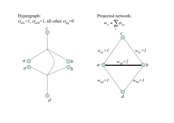
Figure 1: Illustration for the projection $\mathcal{P}_{a}$ from hypergraphs to networks. On the left, a hypergraph is composed of a multitude of hyperedges that exist when $\sigma=1$, and do not when $\sigma=0$. The projected network (right) has a link between all nodes that belong to the same hyperedge, and the weight of the link is the number of hyperedges that share the same pair of nodes.

An illustration of $\mathcal{P}_{a}$ for the case of $r=3$ is shown in Fig. 1.

In the literature, both hypergraphs and projections have been used to study interaction data qualitatively embedded in complex networks theory, but without a sense of unification. For instance, the choice $\mathcal{P}_{n}(O_{ij})$ is implicit in work such as Yoon ; there, if $\sigma_{i_{1},\dots,i_{r}}$ is interpreted as a specific motif (structural pattern), the model generates unweighted networks guaranteed to posses those motifs. In another approach, found in Refs. Newman-clusters ; Miller-clusters , each hypergraph (containing $r=2$ and 3 only) treats each rank separately in that the interactions of nodes by way of pairs is counted independently to the triplet interactions, with no notion of projection onto a simple network. Refs. Ghoshal ; Wasserman do consider projections in some form, but are limited by rank $r$ of hypergraph and by the nature of the projection. Projection $\mathcal{P}_{a}$ is in fact common Wasserman , and it is often used as a way to characterize the one-mode networks that emerge from bipartite graphs fn-bipartite (recent work also uses the notion of projection in the context of time evolving networks Barrat ). Eq. (1) offers a unified way to relate networks and hypergraphs, which can be applied to the models cited above to develop additional understanding of the problems.

To build unbiased statistical models, I adapt to hypergraphs the canonical ensemble approach developed in Ref. Park . The set of all possible hypergraphs $\boldsymbol{\sigma}$ is given by $\{\boldsymbol{\sigma}\}_{\rm conf}$ (the ensemble), or in other words, $\{\boldsymbol{\sigma}\}_{\rm conf}$ is the union of all possible unique hypergraphs $\boldsymbol{\sigma}$. To analytically formulate the ensemble problem, consider the entropy $S$, defined as

$$S=-\sum_{\{\boldsymbol{\sigma}\}_{\rm conf}}P(\boldsymbol{\sigma})\ln P(\boldsymbol{\sigma}),$$ (4)

where $P(\boldsymbol{\sigma})$ represents the probability of a given configuration within the hypergraph ensemble, and the sum over configurations is equivalent to summing over all hyperedge combinations, or $\sum_{\{\boldsymbol{\sigma}\}_{\rm conf}}\rightarrow\sum_{\sigma_{1,\dots,r}=0}^{1}\dots\sum_{\sigma_{N-r+1,\dots,N}=0}^{1}$. The canonical ensemble approach finds the distribution $P(\boldsymbol{\sigma})$ that maximizes $S$ while satisfying conditions that define the ensemble of interest. Such conditions, say $\{\langle X_{\alpha}\rangle\}$, with $\alpha$ an enumeration index, are taken to be of the form

$$\sum_{\{\boldsymbol{\sigma}\}_{\rm conf}}X_{\alpha}(\boldsymbol{\sigma})P(\boldsymbol{\sigma})=\langle X_{\alpha}\rangle.$$ (5)

Finally, since $P(\boldsymbol{\sigma})$ are probabilities, one must guarantee normalization, which translates into

$$\sum_{\{\boldsymbol{\sigma}\}_{\rm conf}}P(\boldsymbol{\sigma})=1.$$ (6)

The solution to this problem ($P(\boldsymbol{\sigma})$ satisfying the conditions above) is obtained via Lagrange multipliers. Each condition is related to a multiplier, and one solves the equations

$$\frac{\partial}{\partial P(\boldsymbol{\sigma})}\left[S+\eta\left(1-\sum_{\{\boldsymbol{\sigma}\}_{\rm conf}}P(\boldsymbol{\sigma})\right)+\sum_{\alpha}\beta_{\alpha}\left(\langle X_{\alpha}\rangle-\sum_{\{\boldsymbol{\sigma}\}_{\rm conf}}X_{\alpha}(\boldsymbol{\sigma})P(\boldsymbol{\sigma})\right)\right]=0,$$ (7)

for $P(\boldsymbol{\sigma})$, with $\eta,\beta_{1},\dots$ the Lagrange multipliers. The solution to the problem can be expressed as

$$P(\boldsymbol{\sigma})=\frac{e^{-H(\boldsymbol{\sigma})}}{Z}.$$ (8)

The partition function $Z$, and $H(\boldsymbol{\sigma})$ (defined as the Hamiltonian), are respectively given by

$$Z=\sum_{\{\boldsymbol{\sigma}\}_{\rm conf}}e^{-H(\boldsymbol{\sigma})}$$ (9)

and

$$H(\boldsymbol{\sigma})=\sum_{\alpha}\beta_{\alpha}X_{\alpha}(\boldsymbol{\sigma}).$$ (10)

Among the simplest non-trivial problems one can address is that of the fully random hypergraph with equal probability for any hyperedge to exist. The constraint associated with this example is the requirement that there is a given average number of hyperedges, $\langle L_{r}\rangle$, over the hypergraph ensemble. Since $L_{r}$ for a given configuration $\boldsymbol{\sigma}$ is given by $L_{r}(\boldsymbol{\sigma})=\sum_{(i_{1},\dots,i_{r})\in\boldsymbol{\sigma}}\sigma_{i_{1},\dots,i_{r}}$, the set of constraints reduces to two Lagrange multipliers, one for the normalization, and another parameter, labelled $\beta$, for $\langle L_{r}\rangle$. Introducing this in Eq. (7) generates the Hamiltonian

$$H(\boldsymbol{\sigma})=\beta\sum_{(i_{1},\dots,i_{r})\in\boldsymbol{\sigma}}\sigma_{i_{1},\dots,i_{r}}=\beta L_{r}(\boldsymbol{\sigma})$$ (11)

and the partition function

$$Z=\sum_{\{\boldsymbol{\sigma}\}_{\rm conf}}e^{-\beta\sum_{(i_{1},\dots,i_{r})\in\boldsymbol{\sigma}}\sigma_{i_{1},\dots,i_{r}}}\\ =\sum_{\sigma_{1,\dots,r}=0}^{1}\dots\sum_{\sigma_{N-r+1,\dots,N}=0}^{1}\prod_{(i_{1},\dots,i_{r})\in\boldsymbol{\rm T}(N,r)}e^{-\beta\sigma_{i_{1},\dots,i_{r}}}\\ =\sum_{\sigma_{1,\dots,r}=0}^{1}e^{-\beta\sigma_{1,\dots,r}}\dots\sum_{\sigma_{N-r+1,\dots,N}=0}^{1}e^{-\beta\sigma_{N-r+1,\dots,N}}=(1+e^{-\beta})^{{N\choose r}},$$ (12)

where $\boldsymbol{\rm T}(N,r)$ is the set of all possible hyperedges $\{(1,\dots,r),\dots,(N-r+1,\dots,N)\}$, i.e., the complete hypergraph of single rank $r$ and size $N$. The last equality can also be obtained from the symmetry of the Hamiltonian over exchange of indices among $\sigma_{i_{1},\dots,i_{r}}$. The result expresses that there are ${N\choose r}$ possible hyperedges $(i_{1},\dots,i_{r})$ among the $N$ nodes. Using this result one can show that the $\langle L_{r}\rangle$ constraint is satisfied for the proper choice of $\beta$, as seen from averaging $L_{r}(\boldsymbol{\sigma})$ in the $P(\boldsymbol{\sigma})$ ensemble

$$\langle L_{r}\rangle=\frac{1}{Z}\sum_{\{\boldsymbol{\sigma}\}_{\rm conf}}\sum_{(i_{1},\dots,i_{r})\in\boldsymbol{\sigma}}\sigma_{i_{1},\dots,i_{r}}e^{-\beta\sum_{(j_{1},\dots,j_{r})\in\boldsymbol{\sigma}}\sigma_{j_{1},\dots,j_{r}}}=\frac{1}{Z}\sum_{L_{r}=0}^{{N\choose r}}{{N\choose r}\choose L_{r}}L_{r}e^{-\beta L_{r}}={N\choose r}p,$$ (13)

and $p\equiv(1+e^{\beta})^{-1}$ is the probability for a hyperedge to be present, which is evident from writing $\langle L_{r}\rangle/{N\choose r}=(1+e^{\beta})^{-1}=p$; $p$ also corresponds to the expectation value of any hyperedge $\langle\sigma_{i_{1},\dots,i_{r}}\rangle=\sum_{\{\boldsymbol{\sigma}\}_{\rm conf}}\sigma_{i_{1},\dots,i_{r}}P(\boldsymbol{\sigma})=(1+e^{\beta})^{-1}=p$, i.e., the probability for any hyperedge to exist. The fact that all hyperedges are equally likely suggests referring to this case as the homogeneous hypergraph ensemble. The probability of a specific hypergraph configuration to be observed is given by Eq. (8), which in this case yields

$$P(\boldsymbol{\sigma},p)=p^{L_{r}(\boldsymbol{\sigma})}(1-p)^{{N\choose r}-L_{r}(\boldsymbol{\sigma})}$$ (14)

where the relations $1+e^{-\beta}=(1-p)^{-1}$ and $e^{-\beta}=p(1-p)^{-1}$ have been used. The application of the $\mathcal{P}_{a}$ and $\mathcal{P}_{n}$ to the homogeneous ensemble is tackled below in a more general ensemble.

The solution to the simple homogeneous problem above, helps to identify some basic features of the canonical approach, including quantities such as the probability of a hyperedge, and of a specific hypergraph $\boldsymbol{\sigma}$. Building on this, one can construct the more general heterogeneous case, where each hyperedge has its own expectation $\langle\sigma_{i_{1},\dots,i_{r}}\rangle$. Thus, the Hamiltonian of Eq. (10) becomes

$$H(\boldsymbol{\sigma})=\sum_{(i_{1},\dots,i_{r})\in\boldsymbol{\sigma}}\beta_{i_{1},\dots,i_{r}}\sigma_{i_{1},\dots,i_{r}}.$$ (15)

In analogy with the homogeneous case, one defines $p_{i_{1},\dots,i_{r}}\equiv\langle\sigma_{i_{1},\dots,i_{r}}\rangle=(1+e^{\beta_{i_{1},\dots,i_{r}}})^{-1}$. The partition function becomes

$$Z(\boldsymbol{\rm p})=\prod_{(i_{1},\dots,i_{r})\in\boldsymbol{\rm T}(N,r)}(1+e^{-\beta_{i_{1},\dots,i_{r}}})=\prod_{(i_{1},\dots,i_{r})\in\boldsymbol{\rm T}(N,r)}(1-p_{i_{1},\dots,i_{r}})^{-1},$$ (16)

where $\boldsymbol{\rm p}$ represents the hyperedge expectations $\{p_{1,\dots,r},\dots,p_{N-r+1,\dots,N}\}$. The probability of a hypergraph configuration $\boldsymbol{\sigma}$ is then

$$P(\boldsymbol{\sigma},\boldsymbol{\rm p})=\prod_{(i_{1},\dots,i_{r})\in\boldsymbol{\rm T}(N,r)}p^{\sigma_{i_{1},\dots,i_{r}}}_{i_{1},\dots,i_{r}}(1-p_{i_{1},\dots,i_{r}})^{1-\sigma_{i_{1},\dots,i_{r}}},$$ (17)

which is the joint probability that hyperedges with $\sigma_{i_{1},\dots,i_{r}}=1$ are present, and those with $\sigma_{i_{1},\dots,i_{r}}=0$ are absent. If for all $(i_{1},\dots,i_{r})\in\boldsymbol{\rm T}(N,r)$, $p_{i_{1},\dots,i_{r}}=p$, one recovers the homogeneous case. The heterogeneous ensemble possesses the most degrees of freedom among non-interacting undirected hypergraph models. If more specific constraints are imposed such as, for instance, conditions on the average number of hyperedges visiting a node, they would translate into additional constraints on the values of the set $\boldsymbol{\rm p}$ (see e.g. discussion at end of Sec. III).

III Application of the hypergraph projection

Since only projections of the form $\mathcal{P}(O_{ij})=\mathcal{P}(o_{ij})$ are considered here, the statistical properties of the projected networks depend on the statistical properties of $o_{ij}$. It is most useful to focus on the distribution of $o_{ij}$ in the heterogeneous ensemble, $\phi_{ij}(o_{ij},\boldsymbol{\rm p})$, and determine how this translates into the homogeneous case (Table 1 summarizes the notation used to compute $\phi_{ij}(o_{ij},\boldsymbol{\rm p})$). Let us define $\boldsymbol{\rm T}_{ij}(N,r)$ as the set of all hyperedges on the complete hypergraph that visit $i$ and $j$ simultaneously. I also define $\overline{\boldsymbol{\rm T}}_{ij}(N,r)$, the complement of $\boldsymbol{\rm T}_{ij}(N,r)$ with respect to $\boldsymbol{\rm T}(N,r)$. In addition, for each configuration $\boldsymbol{\sigma}$, $V_{ij}(\boldsymbol{\sigma})$ is the set of hyperedges visiting $i$ and $j$ which may or may not have cardinality $o_{ij}$ (if it does, it is represented as before with $O_{ij}(\boldsymbol{\sigma})$). The complement of $V_{ij}(\boldsymbol{\sigma})$ with respect to $\boldsymbol{\rm T}_{ij}(N,r)$ is $\overline{V}_{ij}(\boldsymbol{\sigma})$, and thus $\boldsymbol{\rm T}_{ij}(N,r)=V_{ij}(\boldsymbol{\sigma})\bigcup\overline{V}_{ij}(\boldsymbol{\sigma})$. Taking this into account, $\phi_{ij}(o_{ij},\boldsymbol{\rm p})$ can be calculated through the expression

$$\phi_{ij}(o_{ij},\boldsymbol{\rm p})=\sum_{\{\boldsymbol{\sigma}\}_{\rm conf}}\delta\left(o_{ij},\sum_{(i_{1},\dots,i_{r})\in V_{ij}(\boldsymbol{\sigma})}\sigma_{i_{1},\dots,i_{r}}\right)P(\boldsymbol{\sigma},\boldsymbol{\rm p}),$$ (18)

where $\delta(x,y,\dots,z)$ is the Kronecker delta which can have two or more arguments, and is equal to 1 if all the arguments are equal, and 0 otherwise. In the sum above, only those configurations for which delta is 1 contribute to $\phi_{ij}(o_{ij},\boldsymbol{\rm p})$, and this occurs only when there are exactly $o_{ij}$ hyperedges in $\boldsymbol{\sigma}$ that include $ij$.

To perform the calculation, note the independence of each component of $\boldsymbol{\rm p}$ in Eq. (17). This allows factoring the sum over configurations in Eq. (18) into a product of i) the configurations of hyperedges $\overline{\boldsymbol{\rm T}}_{ij}(N,r)$, which cannot affect the delta, and ii) the configurations of hyperedges $\boldsymbol{\rm T}_{ij}(N,r)$, which can. The hyperedges $(i_{1},\dots,i_{r})\in\overline{\boldsymbol{\rm T}}_{ij}(N,r)$ each contribute a factor $\sum_{\sigma_{i_{1}\dots,i_{r}}=0}^{1}p_{i_{1},\dots,i_{r}}^{\sigma_{i_{1},\dots,i_{r}}}(1-p_{i_{1},\dots,i_{r}})^{1-\sigma_{i_{1},\dots,i_{r}}}=1$. Therefore, the remaining factors of Eq. (18) lead to

$$\phi_{ij}(o_{ij},\boldsymbol{\rm p})=\sum_{V_{ij}(\boldsymbol{\sigma})\subset\boldsymbol{\rm V}_{ij}}\delta\left(o_{ij},\sum_{(i_{1},\dots,i_{r})\in V_{ij}(\boldsymbol{\sigma})}\sigma_{i_{1},\dots,i_{r}}\right)\prod_{(i_{1},\dots,i_{r})\in\boldsymbol{\rm T}_{ij}(N,r)}p_{i_{1},\dots,i_{r}}^{\sigma_{i_{1},\dots,i_{r}}}(1-p_{i_{1},\dots,i_{r}})^{1-\sigma_{i_{1},\dots,i_{r}}}\\ =\sum_{V_{ij}(\boldsymbol{\sigma})\subset\boldsymbol{\rm V}_{ij}}\delta\left(o_{ij},\sum_{(i_{1},\dots,i_{r})\in V_{ij}(\boldsymbol{\sigma})}\sigma_{i_{1},\dots,i_{r}}\right)\prod_{(i_{1},\dots,i_{r})\in V_{ij}(\boldsymbol{\sigma})}p_{i_{1},\dots,i_{r}}\prod_{(i_{1},\dots,i_{r})\in\overline{V}_{ij}(\boldsymbol{\sigma})}(1-p_{i_{1},\dots,i_{r}})\\ =\sum_{O_{ij}(\boldsymbol{\sigma})\subset\boldsymbol{\rm O}_{ij}}\prod_{(i_{1},\dots,i_{r})\in O_{ij}(\boldsymbol{\sigma})}p_{i_{1},\dots,i_{r}}\prod_{(i_{1},\dots,i_{r})\in\overline{O}_{ij}(\boldsymbol{\sigma})}(1-p_{i_{1},\dots,i_{r}}),$$ (19)

where $\boldsymbol{\rm V}_{ij}$ and $\boldsymbol{\rm O}_{ij}$ are the unions of all possible sets $V_{ij}(\boldsymbol{\sigma})$ and $O_{ij}(\boldsymbol{\sigma})$, respectively, and $\overline{O}_{ij}(\boldsymbol{\sigma})$ is the complement of $O_{ij}(\boldsymbol{\sigma})$ with respect to $\boldsymbol{\rm T}_{ij}(N,r)$.

Equation (19) has been expressed in a way that makes it straightforward to explain and convert into an algorithm for calculation, as I attempt to explain now. The expression can be described in the following terms: i) separate the hyperedges from $\boldsymbol{\rm T}(N,r)$ into two groups, one that can influence $ij$ over all possible configurations, namely $\boldsymbol{\rm T}_{ij}(N,r)$, and another that cannot ($\overline{\boldsymbol{\rm T}}_{ij}(N,r)$), ii) identify out of $\boldsymbol{\rm T}_{ij}(N,r)$ the hyperedges of $\boldsymbol{\sigma}$ visiting $i$ and $j$, $V_{ij}(\boldsymbol{\sigma})$, iii) only when $|V_{ij}(\boldsymbol{\sigma})|\equiv|O_{ij}(\boldsymbol{\sigma})|=o_{ij}$, $\boldsymbol{\sigma}$ contributes to $\phi_{ij}(o_{ij},\boldsymbol{\rm p})$, and iv) since there are numerous ways to choose $O_{ij}(\boldsymbol{\sigma})$ from $\boldsymbol{\rm T}_{ij}(N,r)$, one requires the set $\boldsymbol{\rm O}_{ij}$, which contains all those choices, i.e., is the ensemble of allowed configurations. Consequently, the last line of Eq. (19) can be read as the sum of probabilities over all possible configurations $\boldsymbol{\rm O}_{ij}$ of hyperedge sets $O_{ij}(\boldsymbol{\sigma})$, where each hyperedge belongs to $\boldsymbol{\rm T}_{ij}(N,r)$. Note that there are $|\boldsymbol{\rm T}_{ij}(N,r)|={N-2\choose r-2}$ hyperedges to choose from and each $O_{ij}(\boldsymbol{\sigma})$ (configuration $\boldsymbol{\sigma}$) picks $o_{ij}$ of them, and therefore $|\boldsymbol{\rm O}_{ij}|={{N-2\choose r-2}\choose o_{ij}}$. It is worth mentioning that $\boldsymbol{\sigma}$ is used in $O_{ij}(\boldsymbol{\sigma})$ to emphasize its origin as a particular hypergraph configuration, but that it becomes redundant when the meaning of $\boldsymbol{\rm O}_{ij}$ is fixed as the collection of configurations (the ensemble) contributing to $\phi_{ij}(o_{ij},\boldsymbol{\rm p})$; at this point, each $O_{ij}$ specifies a unique configuration and no further reference to $\boldsymbol{\sigma}$ is necessary.

In fact, dropping $\boldsymbol{\sigma}$ from $O_{ij}$ offers a combinatorial picture for the last line of Eq. (19) and other distributions in this section. Since each $\boldsymbol{\sigma}$ is a set of hyperedges connecting non-repeated nodes in cliques of rank $r$, one can think of each hyperedge as an $r$-tuple of non-repeated indices taken from $\{1,\dots,N\}$, and a configuration $\boldsymbol{\sigma}$ as a collection of non-repeated $r$-tuples. Therefore, $\boldsymbol{\rm T}(N,r)$ is the collection of all possible $r$-tuples, $\boldsymbol{\rm T}_{ij}(N,r)$ the subset of $\boldsymbol{\rm T}(N,r)$ containing all $r$-tuples that have indices $i$ and $j$ simultaneously, each $O_{ij}$ a sample without replacement of $o_{ij}$ $r$-tuples taken from $\boldsymbol{\rm T}_{ij}(N,r)$, and $\boldsymbol{\rm O}_{ij}$ the collection of all possible samplings. This way to think about Eq. (19) transfers the emphasis from a graph theoretic problem to a purely combinatorial one. The cardinalities of all the sets calculated before follow naturally.

The average of $o_{ij}$ can be determined from Eq. (19), through $\langle o_{ij}(\boldsymbol{\rm p})\rangle=\sum_{o_{ij}=0}^{N-2\choose r-2}o_{ij}\phi(o_{ij},\boldsymbol{\rm p})$, or by calculating $\sum_{\{\boldsymbol{\sigma}\}_{\rm conf}}o_{ij}(\boldsymbol{\sigma})P(\boldsymbol{\sigma})$. The result is

$$\langle o_{ij}(\boldsymbol{\rm p})\rangle=\sum_{(i_{1},\dots,i_{r})\in\boldsymbol{\rm T}_{ij}(N,r)}p_{i_{1},\dots,i_{r}}$$ (20)

which fits intuition, stating that the expectation of the number of hyperedges visiting the pair $ij$, is the sum of expectations of each hyperedge that can visit $ij$ to be present over the ensemble.

In the homogeneous case, where $p_{i_{1},\dots,i_{r}}=p$ for all $(i_{1},\dots,i_{r})$, $\phi_{ij}(o_{ij},\boldsymbol{\rm p})\to\phi_{ij}(o_{ij},p)$ becomes

$$\phi_{ij}(o_{ij},p)={{N-2\choose r-2}\choose o_{ij}}p^{o_{ij}}(1-p)^{{N-2\choose r-2}-o_{ij}},$$ (21)

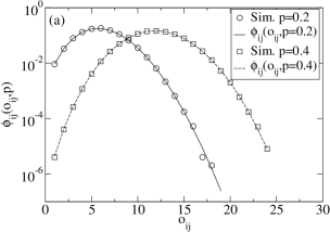
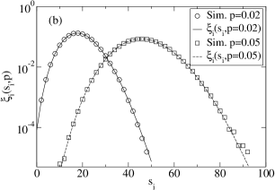
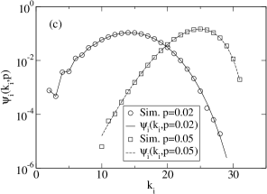
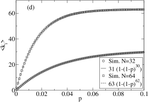
Figure 2: Comparison between theoretical distributions (lines) and simulations (symbols) for distributions of homogeneous projected networks for $N=32$ and $r=3$: (a) $\phi_{ij}(o_{ij},p)$ from Eq. (21) for $N=32$ and corresponding simulations ($\bigcirc$ for $p=0.2$ and $\square$ for $p=0.4$); (b) $\xi_{i}(s_{i},p)$ from Eq. (27) for $N=32$ and corresponding simulation ($\bigcirc$ for $p=0.02$ and $\square$ for $p=0.05$); (c) $\psi_{i}(k_{i},p)$ from Eq. (36) for $N=32$ and corresponding simulations ($\bigcirc$ for $p=0.02$ and $\square$ for $p=0.05$). (d) Average degree $\langle k_{i}\rangle$ as a function of $p$ in homogeneous networks from Eq. (38) and from simulations ($\bigcirc$ for $N=32$ and $\square$ for $N=64$).

a binomial distribution with $\langle o_{ij}\rangle={N-2\choose r-2}p$ (Fig. 2(a)). Both this average, and more generally Eq. (20), have an interesting interpretation explained below regarding signatures of multiway interactions in observational studies. Another noteworthy fact exhibited by Eq. (21), even in this very simple case of homogeneous $p$, is that $o_{ij}$ does not have a fixed value but instead follows a probability distribution consequence of the projection process.

Some general features of $\mathcal{P}$ can now be described if one conditions it to be a monotonic smooth projection, satisfying the inverse function theorem. This condition offers a way to formally write the distribution of $w_{ij}$ from the distribution of $o_{ij}$ because there is a one-to-one relation between the two quantities. Furthermore, one can make use of the monotonicity in both the discrete and continuous variable cases. For the discrete case, defining the distribution $\mu_{ij}(w_{ij},\boldsymbol{\rm p})$ of weights, it is simple to see that $\mu_{ij}(w_{ij},\boldsymbol{\rm p})=\phi_{ij}(\mathcal{P}(o_{ij}),\boldsymbol{\rm p})$ and the set of possible $w_{ij}$ is obtained by applying Eq. (1) to the domain of $o_{ij}$. In the continuous case, introducing the densities $\mu_{ij}(w_{ij},\boldsymbol{\rm p})\to\tilde{\mu}_{ij}(w_{ij},\boldsymbol{\rm p})dw_{ij}$ and $\phi_{ij}(o_{ij},\boldsymbol{\rm p})\to\tilde{\phi}_{ij}(o_{ij},\boldsymbol{\rm p})do_{ij}$, the change of variables theorem for probability distributions implies

$$\tilde{\mu}_{ij}(w_{ij},\boldsymbol{\rm p})=\frac{\tilde{\phi}_{ij}(\mathcal{P}^{-1}(w_{ij}),\boldsymbol{\rm p})}{\mathcal{P}^{\prime}(\mathcal{P}^{-1}(w_{ij}))},$$ (22)

where $\mathcal{P}^{\prime}$ is the derivative of $\mathcal{P}$. The additive projection $\mathcal{P}_{a}$ satisfies monotonicity in a trivial way because it is just the identity function. However, a large class of functions also satisfy monotonicity, including all power law and logarithmic growth functions. The nominal projection, on the other hand, does not satisfy the condition because any value of $o_{ij}\geq 1$ leads to the same weight $w_{ij}=1$, and thus the inverse of $\mathcal{P}_{n}$ is not uniquely defined. Regarding the influence of $\tilde{\phi}_{ij}$, if this distribution is sufficiently narrow in comparison to the shape of $\mathcal{P}$, asymptotic estimates of $\tilde{\mu}_{ij}(w_{ij},p)$ and it properties (e.g., moments) can be straightforwardly obtained.

As I now describe, $\langle o_{ij}(\boldsymbol{\rm p})\rangle$ carries a signature of multiway interactions ($r>2$) that can emerge in a large class of weighted projected networks; if such signature is observed in independently collected weighted network data for which there is no direct observation of multiway interactions, it would be reasonable to suspect the presence of these interactions hidden underneath the weighted network. To explain this, consider Eq. (20) for the ensemble of hypergraphs (although the following results are also valid for a single typical large enough hypergraph) and label $\boldsymbol{\rm p}_{ij}$ the set of probabilities $\{p_{i_{1},\dots,i_{r}}|(i_{1},\dots,i_{r})\in\boldsymbol{\rm T}_{ij}(N,r)\}$ of the hyperedges that visit $ij$, with $\overline{p}_{ij}$ the average and $\Delta p_{ij}$ the variance over the $\boldsymbol{\rm p}_{ij}$ elements. For simplicity, let us assume that $N$ increases to $N+\delta N$, and each new node $N+1,N+2,\dots,N+\delta N$ connects to $ij$ via new hyperedges. Thus, e.g. for nodes $i,j$, and $N+1$ there are ${N+\delta N-3\choose r-3}$ new hyperedges which can potentially occur in a hypergraph, and similarly for all other new nodes. Let us also assume that the total set of hyperedges $\boldsymbol{\rm p}_{ij}+\boldsymbol{\delta}\boldsymbol{\rm p}_{ij}=\{p_{i_{1},\dots,i_{r}}|(i_{1},\dots,i_{r})\in\boldsymbol{T}_{ij}(N+\delta N,r)\}$ after the addition of $\delta N$ has the same average as $\boldsymbol{\rm p}_{ij}$, i.e., $\overline{p_{ij}+\delta p_{ij}}=\overline{p}_{ij}$ and variance $\Delta(p_{ij}+\delta p_{ij})=\Delta p_{ij}$; this is satisfied if the $p_{i_{1},\dots,i_{r}}$ in our model are all drawn from the same distribution. Both $\overline{p}_{ij}$ and $\Delta p_{ij}$ are finite because $0\leq p_{i_{1},\dots,i_{r}}\leq 1$. Under these conditions, the central limit theorem Feller applies to the elements of $\boldsymbol{\rm p}_{ij}+\boldsymbol{\delta}\boldsymbol{\rm p}_{ij}$ and $\boldsymbol{\rm p}_{ij}$. Hence, $\langle o_{ij}(\boldsymbol{\rm p}+\boldsymbol{\delta}\boldsymbol{\rm p})\rangle\to{N+\delta N-2\choose r-2}\overline{p}_{ij}$ asymptotically in $N$. In fact, if every (large enough) subset of $\boldsymbol{\rm p}_{ij}$ is such that $\overline{p}_{ij}$ and $\Delta p_{ij}$ are constant, $\langle o_{ij}(\boldsymbol{\rm p})\rangle\to{N-2\choose r-2}\overline{p}_{ij}$. The set of conditions stipulated above are naturally attained in the heterogeneous hypergraph model, where the elements of $\boldsymbol{\rm p}_{ij}$ can be looked at as independent random variables. The homogeneous case, with all $p_{i_{1},\dots,i_{r}}=p$, satisfies this average exactly even away from the large $N$ limit as seen from the average of Eq. (21).

The relevance of this result lies in the fact that there is a qualitative change in the behavior of $\langle o_{ij}(\boldsymbol{\rm p})\rangle$ for $r=2$ and $r>2$. In the former $\langle o_{ij}(\boldsymbol{\rm p})\rangle\to\overline{p}_{ij}$ which does not scale with $N$, but in the later it scales as $\overline{p}_{ij}N^{r-2}/(r-2)!$ fn-other-quantities ; i.e., $r>2$ makes $\langle o_{ij}(\boldsymbol{\rm p})\rangle$ monotonically increasing with $N$. To appreciate the importance of this, consider a weighted network where one observes that link weights $\langle w_{ij}\rangle$ and size $N$ evolve together with positive correlation (say, both $N$ and the set of $\langle w_{ij}\rangle$ grow together). Two possible qualitative pictures come to mind to explain this behavior: i) the underlying system is in fact composed of a number of multiway interactions that superimpose to produce a weighted network, roughly as described in this article, or ii) the system is pairwise, but the addition of nodes not only introduces edges between each new node and an old existing node, but also the existing nodes tend to strengthen the connections between each other by some additional mechanism. The later model, although possible, is much less natural, and represents a less economical explanation of the correlation between $N$ and link weights. Therefore, being conservative in our interpretation, if $N$ is positively correlated with some or all of the $\langle w_{ij}\rangle$, this should be taken as a first indication that multiway interactions can be present. Note that the absence of correlations between $N$ and $\langle w_{ij}\rangle$ does not exclude the presence of multiway interactions, as specific cases may have additional effects not covered here that may obscure the signatures, e.g., local multiway relations, interactions between hyperedges, etc.

Certainly, one could argue that for there to be a weighted network with the behavior described here, it is also necessary to impose conditions on the type of projection that applies. This is indeed true, but the conditions necessary to obtain correlation between $\langle w_{ij}\rangle$ and $N$ are relatively modest and well justified in numerous circumstances. For instance, here I focus on a monotonically increasing $\mathcal{P}$, which proves sufficient. Furthermore, it is even acceptable to have a $\overline{p}_{ij}$ that decreases with $N$, just as long as the decrease is slower than $N^{-(r-2)}$. The level of detail known about $\mathcal{P}$ and $\boldsymbol{\rm p}_{ij}$ goes hand in hand with the detail that can be learned about the multiway interactions. For instance, if $\overline{p}_{ij}=p$ (homogeneous) and $\mathcal{P}=\mathcal{P}_{a}$, then $\ln\langle w_{ij}\rangle$ vs. $\ln N$ would yield the value of $r$. If, on the other hand, all one knows is that $\mathcal{P}$ is monotonically increasing, the $\ln\langle w_{ij}\rangle$ vs. $\ln N$ would offer an estimate of the combined effects of $\mathcal{P}$ and $\boldsymbol{\rm p}_{ij}$. Overall, the present discussion suggest that in the case of evolving networks with correlations between $N$ and the set of $\langle w_{ij}\rangle$, it is reasonable to suspect multiway interactions active in the background, and further exploration for evidence of such interactions is well justified. These results are general, and do not need to be specialized into a particular example. However, if one is interested in using the results of this article as a method to attempt to determine quantitative details of the multiway interactions that may be present, additional work is needed to extend the results to more detailed and perhaps slightly different situations.

The two projections $\mathcal{P}_{a}$ and $\mathcal{P}_{n}$ can now be explained further. For $\mathcal{P}_{a}$, the properties of $w_{ij}$ are those of $o_{ij}$, and thus already calculated. The other property to describe is the so-called strength $s_{i}$ of node $i$, equal to $\sum_{j}o_{ij}$. It is intuitively helpful to calculate the distribution of strengths $\xi_{i}(s_{i},\boldsymbol{\rm p})$ by making use of the relation between $s_{i}$ and $\ell_{i}$, the number of hyperedges visiting $i$. These two quantities relate via $s_{i}=(r-1)\ell_{i}$, and one can determine the distribution $\zeta_{i}(\ell_{i},\boldsymbol{\rm p})$ of $\ell_{i}$ and from it compute $\xi_{i}(s_{i},\boldsymbol{\rm p})$. Note that while $s_{i}$ is a property of the graph, $\ell_{i}$ is a property of the hypergraph. Once again, the independence of the components of $\boldsymbol{\rm p}$ simplifies the sum over configurations $\{\boldsymbol{\sigma}\}_{\rm conf}$ (notation in Table 2). The hyperedges that could affect $\ell_{i}$ belong to $\boldsymbol{\rm T}_{i}(N,r)$, the collection of all hyperedges visiting $i$ in $\boldsymbol{\rm T}(N,r)$, and $L_{i}(\boldsymbol{\sigma})$ is the set of hyperedges from $\boldsymbol{\rm T}_{i}(N,r)$ in configuration $\boldsymbol{\sigma}$ (when $|L_{i}(\boldsymbol{\sigma})|=\ell_{i}$ one writes it as $\lambda_{i}(\boldsymbol{\sigma})$). From the definition $\zeta_{i}(\ell_{i},\boldsymbol{\rm p})=\sum_{\{\boldsymbol{\sigma}\}_{\rm conf}}\delta(\ell_{i},\sum_{(i_{1},\dots,i_{r})\in L_{i}(\boldsymbol{\sigma})}\sigma_{i_{1},\dots,i_{r}})P(\boldsymbol{\sigma},\boldsymbol{\rm p})$, one can quickly conclude that

$$\zeta_{i}(\ell_{i},\boldsymbol{\rm p})=\sum_{\lambda_{i}(\boldsymbol{\sigma})\in\boldsymbol{\Lambda}_{i}}\prod_{(i_{1},\dots,i_{r})\in\lambda_{i}(\boldsymbol{\sigma})}p_{i_{1},\dots,i_{r}}\prod_{(i_{1},\dots,i_{r})\in\overline{\lambda}_{i}(\boldsymbol{\sigma})}(1-p_{i_{1},\dots,i_{r}}),$$ (23)

where $\boldsymbol{\Lambda}_{i}$ is the ensemble of configurations $\lambda_{i}(\boldsymbol{\sigma})$, and $\lambda_{i}(\boldsymbol{\sigma})\bigcup\overline{\lambda}_{i}(\boldsymbol{\sigma})=\boldsymbol{\rm T}_{i}(N,r)$. Then

$$\xi_{i}(s_{i},\boldsymbol{\rm p})=\zeta_{i}(s_{i}/(r-1),\boldsymbol{\rm p})/(r-1),$$ (24)

where $s_{i}$ takes values $0,r-1,2(r-1),\dots,(r-1){N-1\choose r-1}$. Once again, an equivalence between hyperedge sets and combinatorics can be drawn: $\boldsymbol{\rm T}_{i}(N,r)$ is the union of all $r$-tuples drawn from $\{1,\dots,N\}$ with one element always $i$, and thus there are $|\boldsymbol{\rm T}_{i}(N,r)|={N-1\choose r-1}$ $r$-tuples in total. Each $\lambda_{i}$ is a distinct choice of $\ell_{i}$ of these $r$-tuples; clearly $|\boldsymbol{\Lambda}_{i}|={{N-1\choose r-1}\choose\ell_{i}}$. The sum $\sum_{\lambda_{i}\in\boldsymbol{\Lambda}_{i}}$ is a sum over all choices of $\ell_{i}$ $r$-tuples from $\boldsymbol{\rm T}_{i}(N,r)$. The averages of these quantities are given by

$$\langle\ell_{i}(\boldsymbol{\rm p})\rangle=\sum_{(i_{1},\dots,i_{r})\in\boldsymbol{\rm T}_{i}(N,r)}p_{i_{1},\dots,i_{r}}$$ (25)

and

$$\langle s_{i}(\boldsymbol{\rm p})\rangle=(r-1)\langle\ell_{i}(\boldsymbol{\rm p})\rangle=(r-1)\sum_{(i_{1},\dots,i_{r})\in\boldsymbol{\rm T}_{i}(N,r)}p_{i_{1},\dots,i_{r}}.$$ (26)

For the homogeneous case, $\zeta_{i}(\ell_{i},p)={{N-1\choose r-1}\choose\ell_{i}}p^{\ell_{i}}(1-p)^{{N-1\choose r-1}-\ell_{i}}$, with average $\langle\ell_{i}\rangle={N-1\choose r-1}p$. Therefore,

$$\xi_{i}(s_{i},p)={{N-1\choose r-1}\choose s_{i}/(r-1)}p^{s_{i}/(r-1)}(1-p)^{{N-1\choose r-1}-s_{i}/(r-1)},$$ (27)

and $\langle s_{i}\rangle=(r-1){N-1\choose r-1}p$ (see Fig. 2(b)).

The nominal interaction $\mathcal{P}_{n}$ needs a different treatment. Note that under this projection, $w_{ij}$ can be either 0 or 1. To determine the probability for $w_{ij}$, $\pi_{ij}(w_{ij},\boldsymbol{\rm p})$, one merely needs to determine the probabilities that $o_{ij}$ is either 0 or $\geq 1$, that is $\pi_{ij}(w_{ij},\boldsymbol{\rm p})=\phi_{ij}(o_{ij}=0,\boldsymbol{\rm p})$ or $\pi_{ij}(w_{ij}=1,\boldsymbol{\rm p})=1-\phi_{ij}(o_{ij}=0,\boldsymbol{\rm p})$. Therefore,

$$\pi_{ij}(w_{ij},\boldsymbol{\rm p})=\left\{\begin{array}[]{ll}1-\prod_{(i_{1},\dots,i_{r})\in\boldsymbol{\rm T}_{ij}(N,r)}(1-p_{i_{1},\dots,i_{r}});&\qquad w_{ij}=1\\ \prod_{(i_{1},\dots,i_{r})\in\boldsymbol{\rm T}_{ij}(N,r)}(1-p_{i_{1},\dots,i_{r}});&\qquad w_{ij}=0.\end{array}\right.$$ (28)

In the homogeneous case,

$$\pi_{ij}(w_{ij},p)=\left\{\begin{array}[]{ll}1-(1-p)^{N-2\choose r-2};&\qquad w_{ij}=1\\ (1-p)^{N-2\choose r-2};&\qquad w_{ij}=0.\end{array}\right.$$ (29)

Both Eqs. (28) and (29) are closely related to the average number of connections for each node of a projected network, as explained next.

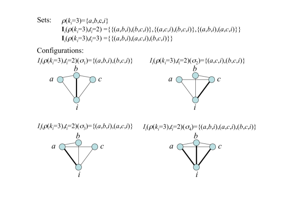
Figure 3: Illustration ($r=3$) of the emergence of degree $k_{i}$ as a consequence of various possible hyperedge configurations. The figure also illustrates $Q_{r-1}(k_{i},\ell_{i})$. There are 4 possible ways in which $i$ can be connected to nodes $\{a,b,c\}$, each case corresponding to one of the configurations shown above ($\boldsymbol{\sigma}_{1},\boldsymbol{\sigma}_{2},\boldsymbol{\sigma}_{3},\boldsymbol{\sigma}_{4}$) in the projected network. The sets $\boldsymbol{\rm I}_{i}(\rho(k_{i}),\ell_{i})$ are defined for both $\ell_{i}=2$ and 3, the only two possible cases. Note also that if one focuses only on the nodes $\{a,b,c\}$ ignoring $i$, all configurations can be mapped to the construction of all possible cliques of size 2 of these nodes, generating $Q_{r-1=2}(k_{i}=3,\ell_{i}=2)=3$ and $Q_{r-1=2}(k_{i}=3,\ell_{i}=3)=1$. The fact that all configurations are globally connected is an accident due to the small value of $k_{i}=3$, but in general, nodes simply need to belong to $\ell_{i}$ cliques of size $r-1$. Finally, note the thickness of links, representative of $o_{ij}$.

For any weighted projected network generated from a $\mathcal{P}$ satisfying $o_{ij}>0\Rightarrow w_{ij}>0$ and $o_{ij}=0\Rightarrow w_{ij}=0$, such as $\mathcal{P}_{a}$ and $\mathcal{P}_{n}$, the number of connections $k_{i}$ visiting node $i$ are characterized by $\psi_{i}(k_{i},\boldsymbol{\rm p})$, the distribution of $k_{i}$ (an expanded and pedagogical exposition of the calculation and its consequences can be found in Lopez-pk ). The degree can be either 0 or take any value from $r-1\leq k_{i}\leq N-1$. To determine $\psi_{i}(k_{i},\boldsymbol{\rm p})$ (notation in Table 3), one can proceed in a similar way as before: in configuration $\boldsymbol{\sigma}$, the set of hyperedges visiting $i$ and producing degree $k_{i}$ is $K_{i}(\boldsymbol{\sigma})$. This means that hyperedges in $K_{i}(\boldsymbol{\sigma})$ visit exactly $k_{i}$ nodes and node $i$. It is interesting to note that another configuration $\boldsymbol{\sigma}^{\prime}$, associated with $K_{i}(\boldsymbol{\sigma}^{\prime})$, with a different set and/or number of hyperedges can lead to the same $k_{i}$, because these hyperedges still visit the same number of nodes $k_{i}$ (see Fig. 3 for an illustration). With this definition, one can write

$$\psi_{i}(k_{i},\boldsymbol{\rm p})=\sum_{K_{i}(\boldsymbol{\sigma})\in\boldsymbol{\rm K}_{i}}\prod_{(i_{1},\dots,i_{r})\in K_{i}(\boldsymbol{\sigma})}p_{i_{1},\dots,i_{r}}\prod_{(i_{1},\dots,i_{r})\in\overline{K}_{i}(\boldsymbol{\sigma})}(1-p_{i_{1},\dots,i_{r}}),$$ (30)

where $\boldsymbol{\rm K}_{i}$ is the union of all possible sets $K_{i}(\boldsymbol{\sigma})$, and the complement set $\overline{K}_{i}(\boldsymbol{\sigma})$ satisfies $K_{i}(\boldsymbol{\sigma})\bigcup\overline{K}_{i}(\boldsymbol{\sigma})=\boldsymbol{\rm T}_{i}(N,r)$. Since the number of hyperedges is not fixed across members of $\boldsymbol{\rm K}_{i}$, one can further organize the $K_{i}(\boldsymbol{\sigma})$ by their numbers of hyperedges $\ell_{i}(\boldsymbol{\sigma})$. The bounds of $\ell_{i}$ are dictated by the following: for degree $k_{i}$, a minimum of $\lceil k_{i}/(r-1)\rceil$ hyperedges is required ($\lceil.\rceil$ represents the ceiling function), and there can be no more than ${k_{i}\choose r-1}$ hyperedges. Using this organization, and introducing the notation $K^{(\ell_{i})}_{i}(\boldsymbol{\sigma})$ and $\boldsymbol{\rm K}_{i}(\ell_{i})$ to represent, respectively, the sets $K_{i}(\boldsymbol{\sigma})$ involving exactly $\ell_{i}$ hyperedges and their unions, one can write

$$\psi_{i}(k_{i},\boldsymbol{\rm p})=\sum_{\ell_{i}=\left\lceil\frac{k_{i}}{r-1}\right\rceil}^{k_{i}\choose r-1}\sum_{K^{(\ell_{i})}_{i}(\boldsymbol{\sigma})\in\boldsymbol{\rm K}_{i}(\ell_{i})}\prod_{(i_{1},\dots,i_{r})\in K^{(\ell_{i})}_{i}(\boldsymbol{\sigma})}p_{i_{1},\dots,i_{r}}\prod_{(i_{1},\dots,i_{r})\in\overline{K}^{(\ell_{i})}_{i}(\boldsymbol{\sigma})}(1-p_{i_{1},\dots,i_{r}}).$$ (31)

The sets $\boldsymbol{\rm K}_{i}(\ell_{i})$ are only subsets of $\boldsymbol{\Lambda}_{i}$ in which the $\ell_{i}$ hyperedges involve exactly $i$ and $k_{i}$ other nodes. Finally, it is possible to exploit one more symmetry that facilitates an algorithmic understanding of $\psi_{i}(k_{i},\boldsymbol{\rm p})$: the sets that make up $\boldsymbol{\rm K}_{i}(\ell_{i})$ involve several possible distinct node sets. However, one can further segregate these sets by the specific nodes in them. Hence, if one takes a set, $\rho(k_{i})$, of $k_{i}$ specific nodes and $i$, there are several configurations in which their associated $K^{(\ell_{i})}_{i}(\boldsymbol{\sigma})$ contain $\ell_{i}$ hyperedges visiting only those nodes. Thus, a configuration with specific $\rho(k_{i})$ nodes connected to $i$, using $\ell_{i}$ hyperedges is labelled $I^{(\rho(k_{i}),\ell_{i})}_{i}(\boldsymbol{\sigma})$, and the union of configurations is labelled $\boldsymbol{\rm I}_{i}(\rho(k_{i}),\ell_{i})$. The union of all sets $\boldsymbol{\rm I}_{i}(\rho(k_{i}),\ell_{i})$ (which are non-intersecting) is equal to $\boldsymbol{\rm K}_{i}(\ell_{i})$. This leads to the final expression

$$\psi_{i}(k_{i},\boldsymbol{\rm p})=\sum_{\rho(k_{i})\in\boldsymbol{\rm R}_{i}(N,k_{i})}\\ \sum_{\ell_{i}=\left\lceil\frac{k_{i}}{r-1}\right\rceil}^{k_{i}\choose r-1}\sum_{I^{(\rho(k_{i}),\ell_{i})}_{i}(\boldsymbol{\sigma})\in\boldsymbol{\rm I}_{i}(\rho(k_{i}),\ell_{i})}\prod_{(i_{1},\dots,i_{r})\in I^{(\rho(k_{i}),\ell_{i})}_{i}(\boldsymbol{\sigma})}p_{i_{1},\dots,i_{r}}\prod_{(i_{1},\dots,i_{r})\in\overline{I}^{(\rho(k_{i}),\ell_{i})}_{i}(\boldsymbol{\sigma})}(1-p_{i_{1},\dots,i_{r}}),$$ (32)

where $\overline{I}^{(\rho(k_{i}),\ell_{i})}_{i}(\boldsymbol{\sigma})$ is the complement of $I^{(\rho(k_{i}),\ell_{i})}_{i}(\boldsymbol{\sigma})$ with respect to $\boldsymbol{\rm T}_{i}(N,r)$, and $\boldsymbol{\rm R}_{i}(N,k_{i})$ is the union of all possible $\rho(k_{i})$, each one a distinct $(k_{i}+1)$-tuple taken from the set $\{1,\dots,N\}$ with one choice always being $i$. The sizes of sets are: $|\boldsymbol{\rm R}_{i}(N,k_{i})|={N-1\choose k_{i}}$, and $|\boldsymbol{\rm I}_{i}(\rho(k_{i}),\ell_{i})|=Q_{r-1}(k_{i},\ell_{i})$; the later is the result of a combinatorial problem that can be defined in terms of general graph theory. Specifically, $Q_{r-1}(k_{i},\ell_{i})$ corresponds to the number of distinct hypergraphs that can be constructed with $k_{i}$ nodes and $\ell_{i}$ hyperedges of rank $r-1$, and each node belongs to at least one of the hyperedges Lopez-pk . In fact, each $I^{(\rho(k_{i}),\ell_{i})}_{i}(\boldsymbol{\sigma})$ can be mapped to each one of these hypergraphs. To determine $\langle k_{i}(\boldsymbol{\rm p})\rangle$, it is convenient to use the relation

$$\langle k_{i}(\boldsymbol{\rm p})\rangle=\sum_{\{\boldsymbol{\sigma}\}_{\rm conf}}k_{i}(\boldsymbol{\sigma})P(\boldsymbol{\sigma})=\sum_{\{\boldsymbol{\sigma}\}_{\rm conf}}\sum_{j=1;j\neq i}^{N}\theta(o_{ij}(\boldsymbol{\sigma}))P(\boldsymbol{\sigma})=\sum_{j=1;j\neq i}^{N}\sum_{\{\boldsymbol{\sigma}\}_{\rm conf}}\theta(o_{ij}(\boldsymbol{\sigma}))P(\boldsymbol{\sigma}).$$ (33)

By first summing over a single $j$, one notices that only hyperedges in $\boldsymbol{\rm T}_{ij}(N,r)$ must be considered in detail. Given that

$$\theta(o_{ij}(\boldsymbol{\sigma}))=\theta\left(\sum_{(i_{1},\dots,i_{r})\in O_{ij}(\boldsymbol{\sigma})}\sigma_{i_{1},\dots,i_{r}}\right)=1-\delta\left(\sum_{(i_{1},\dots,i_{r})\in O_{ij}(\boldsymbol{\sigma})}\sigma_{i_{1},\dots,i_{r}},0\right),$$ (34)

one arrives at

$$\langle k_{i}(\boldsymbol{\rm p})\rangle=\sum_{j=1;j\neq i}^{N}\left[1-\prod_{(i_{1},\dots,i_{r})\in\boldsymbol{\rm T}_{ij}(N,r)}(1-p_{i_{1},\dots,i_{r}})\right].$$ (35)

When compared with Eq. (28), it becomes evident that each link $ij$ contributes to $k_{i}$ independently.

In the homogeneous case, making use of the combinatorial results presented, one obtains (Fig. 2(c))

$$\psi_{i}(k_{i},p)={N-1\choose k_{i}}\sum_{\ell_{i}=\left\lceil\frac{k_{i}}{r-1}\right\rceil}^{k_{i}\choose r-1}Q_{r-1}(k_{i},\ell_{i})p^{\ell_{i}}(1-p)^{{N-1\choose r-1}-\ell_{i}}.$$ (36)

Without diving into too much detail, $Q_{r-1}(k_{i},\ell_{i})$ can be calculated via the inclusion-exclusion principle of combinatorics Riordan ; Lopez-pk , which produces

$$Q_{r-1}(k_{i},\ell_{i})=\sum_{m=0}^{k_{i}}(-1)^{k_{i}-m}{k_{i}\choose m}{{m\choose r-1}\choose\ell_{i}}.$$ (37)

Among the identities satisfied by $Q_{r-1}(k,\ell)$ Lopez-pk , one finds that ${{N-1\choose r-1}\choose\ell}=\sum_{k}{N-1\choose k}Q_{r-1}(k,\ell)$, which is used to show normalization of $\psi_{i}(k_{i},p)$. Another identity, $\sum_{k}k{N-1\choose k}Q_{r-1}(k,\ell)=(N-1)\left[{{N-1\choose r-1}\choose\ell}-{{N-2\choose r-1}\choose\ell}\right]$, leads to the average of $\psi_{i}(k_{i},p)$,

$$\langle k_{i}\rangle=(N-1)\left[1-(1-p)^{N-2\choose r-2}\right],$$ (38)

where the brackets are equal to $\pi_{ij}(w_{ij}=1,p)$ from Eq. (29) (see Fig. 2(d)). This average can also be calculated directly from Eq. (35) Lopez-pk .

To conclude this section, it is useful to point out how the previous results can be connected with concrete problems. The logic is similar to that found in Park ; Bradde , in which the ensemble is chosen to fit observations. In the framework presented here, it is possible to choose the hypergraph ensemble to fit hypergraph properties (such as Eqs. (20) or (25)), projected network properties (Eqs. (26) or (35)), or a combination of both (as long as it is well defined); the choice comes down to practical considerations such as the available data one intends to fit, or the belief that certain mechanisms may be at play and therefore must be part of the model. Once an ensemble is defined (satisfying the assumptions of hyperedges which are non-interacting, undirected, and with uniform rank), the expressions derived above for the heterogeneous ensemble apply, but an additional set of constraints emerges for the $p_{i_{1},\dots,i_{r}}$ guaranteeing that the entropy is maximized, distinguishing the situation from that of the fully heterogeneous ensemble, where each $p_{i_{1},\dots,i_{r}}$ is free to have any value between 0 and 1.

As an example, consider the ensemble that specifies strengths $\langle s_{i}\rangle$ on the projected networks with projection $\mathcal{P}_{a}$. This can be constructed from the Hamiltonian

$$H(\boldsymbol{\sigma})=\sum_{i=1}^{N}\beta_{i}s_{i}(\boldsymbol{\sigma})=(r-1)\sum_{(i_{1},\dots,i_{r})\in\boldsymbol{\sigma}}(\beta_{i_{1}}+\dots+\beta_{i_{r}})\sigma_{i_{1},\dots,i_{r}}.$$ (39)

This ensemble is completely specified by calculating the relation between $\langle\sigma_{i_{1},\dots,i_{r}}\rangle$, by definition equal to $p_{i_{1},\dots,i_{r}}$, and the set of parameters $\{\beta_{1},\dots,\beta_{N}\}$. After determining $P(\boldsymbol{\sigma})$, one can compute $\langle\sigma_{i_{1},\dots,i_{r}}\rangle=\sum_{\{\boldsymbol{\sigma}\}_{\rm conf}}\sigma_{i_{1},\dots,i_{r}}P(\boldsymbol{\sigma})$ to find

$$\langle\sigma_{i_{1},\dots,i_{r}}\rangle=p_{i_{1},\dots,i_{r}}=\frac{e^{-(r-1)(\beta_{i_{1}}+\dots+\beta_{i_{r}})}}{1+e^{-(r-1)(\beta_{i_{1}}+\dots+\beta_{i_{r}})}}$$ (40)

where the parameters satisfy Eq. (26), and therefore

$$\langle s_{i}\rangle=(r-1)\sum_{(i_{1},\dots,i_{r})\in\boldsymbol{\rm T}_{i}(N,r)}p_{i_{1},\dots,i_{r}}=(r-1)\sum_{(i_{1},\dots,i_{r})\in\boldsymbol{\rm T}_{i}(N,r)}\frac{e^{-(r-1)(\beta_{i_{1}}+\dots+\beta_{i_{r}})}}{1+e^{-(r-1)(\beta_{i_{1}}+\dots+\beta_{i_{r}})}}.$$ (41)

One way to understand this result is from the relation

$$dp_{i_{1},\dots,i_{r}}=-(r-1)\sum_{g=1}^{r}\frac{p_{i_{1},\dots,i_{r}}}{1-p_{i_{1},\dots,i_{r}}}d\beta_{i_{g}}.$$ (42)

If only $\beta_{i_{g}}$ changes (by, say, $d\beta_{i_{g}}$), hyperedges without node $i_{g}$ are unaffected, and those with $i_{g}$ all increase in probability proportionally to $d\beta_{i_{g}}$. As in Ref. Park , the $\beta_{i}$ can be taken from a distribution, leading in turn to a distribution of $\langle s_{i}\rangle$. This can be used to obtain a desired distribution of $\langle s_{i}\rangle$ as dictated by the problem.

IV Percolation properties and sparse cases

Another important aspect of the hypergraph ensemble and its projected networks is their percolation properties. To calculate these, one can use the equivalence, first pointed out by Fortuin and Kasteleyn Fortuin , between percolation and the mean-field $q$-states Potts model at $q\to 1$. The solution to the later model consists of determining the state of the nodes, and whether there is a phase transition. The solution and its properties can be obtained by studying the model’s Helmholtz free energy. A detailed development of equivalence of the models can be found in Refs. Bradde ; Engel ; here, I set up the calculation starting at the free energy and develop the percolation properties from there. I consider the homogeneous case only, although it is possible to solve some forms of heterogeneous models.

Consider the Hamiltonian of the general $q$-state Potts model with $N$ nodes, $H_{q}=-\sum_{i_{1},\dots,i_{r}}J_{i_{1},\dots,i_{r}}\delta(u_{i_{1}},\dots,u_{i_{r}})$, where $u_{i_{1}},\dots,u_{i_{r}}$ represent the respective spin states of the nodes $i_{1},\dots,i_{r}$ from the possible states $1,\dots,q$, and $J_{i_{1},\dots,i_{r}}$ the strength of the interaction among them. A hyperedge exists among nodes $i_{1},\dots,i_{r}$ if $u_{i_{1}}=\dots=u_{i_{r}}$, i.e., if these nodes are in the same spin state. Let us denote the number of system nodes with spin $u$ as $N_{u}$, and the density of these as $c_{u}=N_{u}/N$, which satisfies $\sum_{u}c_{u}=1$. In the homogeneous system, since $J_{i_{1},\dots,i_{r}}=J$ and given that only $r$-tuples of equal spins contribute to $H_{q}$ (i.e., only hyperedges), the energy is equal to $H_{q}=-J\sum_{u}{N_{u}\choose r}$, the sum of interaction energies among all hyperedges having equal spin. The connection between percolation and the Potts model carries with it the relation $J=-\ln(1-p)$, and for small $p$, this approximates to $J\approx p$.

In order to find the Helmholtz free energy of the system, one must first determine the partition function $Z_{q}$. In this model, it can be written on the basis of all configurations of state values $u_{i}$, or in terms of the set of numbers $\{N_{u}\}_{u=1,\dots,q}$. Using the later set of variables, and taking into account the multiplicity in the choices for each node state, one arrives at

$$Z_{q}=\sum_{\sum_{u=1}^{q}N_{u}=N}e^{-\left[-J\sum_{u}{N_{u}\choose r}\right]}\frac{N!}{\prod_{u=1}^{q}N_{u}!}=\sum_{\sum_{u=1}^{q}c_{u}=1}e^{-\left[-J\sum_{u}{Nc_{u}\choose r}+N\sum_{u}c_{u}\ln c_{u}\right]},$$ (43)

where the inverse temperature parameter $\beta$ is absorbed into $J$. In the canonical ensemble, the free energy is given by $F_{q}=-\ln Z_{q}$. When the interaction $J$ is too weak to keep the nodes ordered collectively in groups of common states, the solution to the problem is expected to be symmetric, i.e. $c_{u}=1/q$ (all states are equally occupied). However, as the interaction strengthens, one would expect that symmetry is broken and one state (say $u=1$) becomes dominant. By these arguments, $F_{q}$ can be sought by introducing the ansatz

$$c_{u}=\left\{\begin{array}[]{lr}\frac{1+(q-1)\tilde{f}_{q}}{q}&\qquad;u=1{}\\ \frac{1-\tilde{f}_{q}}{q}&\quad;u\neq 1,\end{array}\right.$$ (44)

where $\tilde{f}_{q}$ is the fractional size of the system in state $u=1$, and the condition $\sum_{u}c_{u}=1$ is automatically satisfied. This leads to

$$Z_{q}=\int d\tilde{f}_{q}e^{\left[J{\frac{N}{q}(1+(q-1)\tilde{f}_{q})\choose r}+J(q-1){\frac{N}{q}(1-\tilde{f}_{q})\choose r}-\frac{N}{q}(1+(q-1)\tilde{f}_{q})\ln\frac{1+(q-1)\tilde{f}_{q}}{q}-\frac{N}{q}(1-\tilde{f}_{q})\ln\frac{1-\tilde{f}_{q}}{q}\right]}.$$ (45)

In the thermodynamic limit ($N\to\infty$), the Laplace method of integration can be applied to $Z_{q}$ Bender . Once applied, $F_{q}=-\ln Z_{q}$ yields to leading order

$$F_{q}=-J{\frac{N}{q}(1+(q-1)f_{q})\choose r}-J(q-1){\frac{N}{q}(1-f_{q})\choose r}\\ +\frac{N}{q}(1+(q-1)f_{q})\ln\frac{1+(q-1)f_{q}}{q}+\frac{N}{q}(1-f_{q})\ln\frac{1-f_{q}}{q}$$ (46)

where $f_{q}$ is the value of $\tilde{f}_{q}$ for which the exponent of the argument of the $Z_{q}$ integral is maximized. Explicitly, $f_{q}$ is obtained by equating to 0 the first derivative with respect to $\tilde{f}_{q}$ of the exponent in Eq. (45), and using $c_{1}(f_{q})$ and $c_{u}(f_{q})$ to refer to the the fractions $c_{u}$ from Eq. (44) evaluated at $u=1$ and $u\neq 1$, respectively. Thus, $f_{q}$ must satisfy

$$\ln\left(\frac{1-f_{q}}{1-(q-1)f_{q}}\right)=-J\left[{Nc_{1}(f_{q})\choose r}\sum_{i=1}^{r-1}\frac{1}{Nc_{1}(f_{q})-i}-{Nc_{u}(f_{q})\choose r}\sum_{i=1}^{r-1}\frac{1}{Nc_{u}(f_{q})-i}\right].$$ (47)

This is the self-consistency equation for the fractional size of the component of broken symmetry. For $q=1$, $f\equiv f_{q=1}$ is the fractional size of the percolating spanning cluster. Note that $f_{q}=0$ is also a solution to Eq. (47), but its stability breaks down when the second derivative of the exponent of the integrand of $Z_{q}$ changes sign. The value of $J$ for which the sign change occurs is given by the relation

$$p_{c}\approx J_{c}=\left[N\frac{\partial^{2}}{\partial N^{2}}{N\choose r}\right]^{-1},$$ (48)

where $q=1$ has already been introduced (otherwise the solution would be the same but with $N/q$ in place of $N$ everywhere).

In the thermodynamic limit, one can derive a compact equation for $f$ and arbitrary $r$. Both terms in the brackets of Eq. (47) are polynomials emerging from the derivative $\frac{\partial}{\partial x}{x\choose r}$, labeled $M(x,r)=\sum_{m=0}^{r-1}a_{r}(m)x^{m}$, evaluated at $x=Nc_{1}$ and $Nc_{u}$ (I continue the same shorthand of $c_{u\neq 1}=c_{u}$). Subtracting, one obtains $M(N_{1},r)-M(N_{u\neq 1},r)=\sum_{m=1}^{r-1}a_{r}(m)(N_{1}^{m}-N_{u}^{m})$, where the coefficient $m=0$ vanishes. It is possible to express the coefficients $a_{r}(m)$ in terms of elementary symmetric polynomials MacMahon and binomial coefficients, but the analysis here is restricted to the asymptotic limit, and thus only requires the coefficient $a_{r}(r-1)$, equal to $1/(r-1)!$ as can be determined by inspecting $M(x,r)$. Using the identity $x^{m}-y^{m}=(x-y)\sum_{l=0}^{m-1}x^{m-1-l}y^{l}$, the ansatz (44), and the self-consistency relation (47) with $q=1$, one obtains

$$\ln(1-f)=-Jf\sum_{m=1}^{r-1}a_{r}(m)N^{m}\sum_{l=0}^{m-1}(1-f)^{l}=-J\sum_{m=1}^{r-1}a_{r}(m)N^{m}\left(1-(1-f)^{m}\right).$$ (49)

Close to percolation, it is justified to write $J=\lambda J_{c}$, with $\lambda\geq 1$ and $J_{c}$ from Eq. (48). By L’Hopital’s rule, for the dominant term in $N$, the size of the largest component emerges as

$$\ln(1-f)=-\frac{\lambda}{r-1}(1-(1-f)^{r-1}),$$ (50)

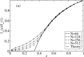
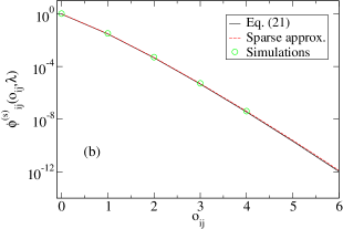
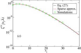
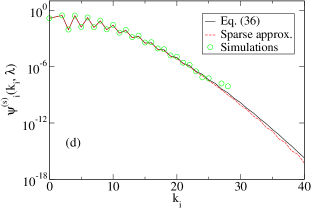
Figure 4: (color online) Percolation limit for the ensemble of $\langle s\rangle=\lambda_{\text{max}}$: (a) $f(z)/f(z=1)$ vs. $z$ ($\lambda_{\text{max}}=3.0$) from Eq. (50) (line) and simulations of $N=64\quad(\bigcirc)$, $N=128\quad(\square)$, $N=256\quad(\Diamond)$ and $N=512\quad(\vartriangle)$. As the system size increases, the theoretical solution is approached. Projected network properties ($\mathcal{P}_{a}$ for $s_{i}$) for $N=128$ in the ensemble of $\langle s\rangle=\lambda=4.0$ predicted by theory (line), their respective sparse approximations (dashed line) and simulations ($\bigcirc$): (b) $\phi^{(s)}_{ij}(o_{ij},\lambda)$,(c) $\xi^{(s)}_{i}(s_{i},\lambda)$, and(d) $\psi^{(s)}_{i}(k_{i},\lambda)$.

which generalizes expressions for $f$ for $r=2$ and 3 in Refs. Newman-clusters ; Miller-clusters (these authors tackle the percolation question to illustrate ideas different than those explored here). To test this expression, it is customary to define the percolation problem with respect to a network (or hypergraph) that is not complete, but instead is already diluted. By defining the rescaling $z=p/p_{\text{max}}$ where typically $p_{\text{max}}\ll 1$, the original undiluted hypergraph is $z=1$, and percolation occurs at $z_{c}=p_{c}/p_{\text{max}}$, or if using $\lambda_{\text{max}}$, $z_{c}=1/\lambda_{\text{max}}$ (see Fig 4(a)).

The percolation transition can be shown to be second order by expanding both sides of Eq. (50), which leads to

$$\sum_{g=1}^{\infty}\frac{f^{g}}{g}=\frac{\lambda}{r-1}\sum_{g^{\prime}=1}^{r-1}{r-1\choose g^{\prime}}(-1)^{g^{\prime}+1}f^{g^{\prime}}.$$ (51)

For small $f$, close to the percolation transition, only the first few terms on both sides of the equality are relevant. Retaining up to second order

$$1+\frac{f}{2}\approx\frac{\lambda}{r-1}\left[(r-1)-{r-1\choose 2}f\right]$$ (52)

which produces

$$f\sim\frac{2(\lambda-1)}{1+(r-2)\lambda}\sim 2(\lambda-1)$$ (53)

clearly indicating a continuous transition, in the same universality class of regular network percolation, which diverges at the transition with exponent 1. This result is known in the literature Newman-clusters .

The previous results focus on hypergraphs, but their relevance to projected networks is not explicitly clear. To clarify this, it is sufficient to explore the properties of $\phi_{ij}(o_{ij},p)$. For this, it is useful to have in mind the asymptotic relations $N\frac{\partial^{2}}{\partial N^{2}}{N\choose r}\sim\frac{N^{r-1}}{(r-2)!}$ and ${N-1\choose r-1}\sim\frac{N^{r-1}}{(r-1)!}$. Inserting $p=\lambda p_{c}$ in Eq. (21), and taking the limit $N\gg o_{ij}$, the relation $\phi_{ij,\text{sparse}}(o_{ij},\lambda p_{c})\equiv\phi^{(s)}_{ij}(o_{ij},\lambda)=(\lambda/N)^{o_{ij}}e^{\lambda/N}/o_{ij}!$, which is a Poisson distribution with average $\lambda/N$ (Fig. 4(b)). Therefore, as $N$ increases, the weights on the links vanish, signalling the fact that in this dilute regime, the hypergraph and projected networks are virtually the same, and hyperedges are non-overlapping asymptotically. Thus, one only needs to calculate the hypergraph percolation properties to be able to write down the projected network percolation properties. In this sparse regime, the other distributions discussed above have particular forms: for the hypergraph, the distribution of hyperedges visiting a node becomes $\zeta^{(s)}_{i}(\ell_{i},\lambda)=(\lambda/(r-1))^{\ell_{i}}e^{-\lambda/(r-1)}/\ell_{i}!$ (poisson with average $\lambda/(r-1)$), and the strength distribution on projected networks with $\mathcal{P}_{a}$ becomes $\xi^{(s)}_{i}(s_{i},\lambda)=(\lambda/(r-1))^{s_{i}/(r-1)}e^{-\lambda/(r-1)}/[(r-1)(s_{i}/(r-1))!]$ (Fig. 4(c)). From these results, the meaning of $\lambda$ emerges as the parameter that measures the average node strength of the projected network. Finally, the degree distribution can be calculated if one keeps in mind that in the sparse limit, the probability that hyperedges overlap is minimal, and therefore, one expects that only the minimum number of hyperedges $\ell_{i}\to\lceil k_{i}/(r-1)\rceil$ contribute to the distribution. There are subtleties present in explicitly calculating $Q_{r-1}(k_{i},\lceil k_{i}/(r-1)\rceil)$ and $\psi^{(s)}_{i}(k_{i},\lambda)$ when $k_{i}$ is not a multiple of $r-1$ because hyperedges are forced to overlap in this case, and thus to avoid further details, I only write the unevaluated result $\psi^{(s)}_{i}(k_{i},\lambda)=Q_{r-1}(k_{i},\lceil k_{i}/(r-1)\rceil)(\lambda p_{c})^{\lceil k_{i}/(r-1)\rceil}(1-\lambda p_{c})^{{N-1\choose r-1}-\lceil k_{i}/(r-1)\rceil}$ (Fig. 4(d)). However, the calculations are not prohibitive, and are derived in detail in Lopez-pk .

The sparse regime close to percolation is not the only possible sparse regime. To be concrete, note that for $p$ close to $p_{c}$, the average node strength is constant, but the average overlap on projected links scales as $N^{-1}$, so the larger the network, the less interaction present along the links. However, one can consider a regime in which $\langle o_{ij}\rangle\sim\lambda/N$ is constant, and in this regime node strength increases with $N$. Both of these regimes are “sparse” in the sense that $p$ vanishes asymptotically, but each regime has specific properties. Generally, these sparse regimes can be defined based on any sensible property, and lead to interesting behavior. Finally, for the dense regime ($p$ constant), the interesting effect of growth of $\langle o_{ij}\rangle$ vs. $N$ emerges, which is a unique feature of this model, and the signature that multiway interactions are potentially present.

V Conclusions

In conclusion, in this article I present a model of hypergraphs and associated weighted projected networks that offers a concise and intuitive picture of hypergraphs, networks, and weights. By using statistical mechanics concepts, together with combinatorial tools, I have been able to determine some basic features of homogeneous and heterogeneous projected networks that offer concrete tests to determine whether a network that has been empirically measured may bear the signature of multiway (group) interactions. The general idea of using the projection of a hypergraph onto a network, which has not been studied systematically to the author’s knowledge until this article, deserves a close look to determine further properties that can help give a better understanding of the genuine limits and virtues of pairwise simplifications in network research.

The author thanks L. Roberts, A. Gerig, F. Reed-Tsochas, and O. Riordan, for helpful discussions, and TSB/EPSRC grant SATURN (TS/H001832/1), ICT eCollective EU project (238597), and the James Martin 21st Century Foundation Reference no: LC1213-006 for financial support.

Set notation	Explanation	Type of element	Size
$\boldsymbol{\rm T}_{ij}(N,r)$	Hyperedges of complete hypergraph simultaneously visiting $i$ and $j$	hyperedge	${N-2\choose r-2}$
$O_{ij}(\boldsymbol{\sigma})$	Hyperedges of configuration $\boldsymbol{\sigma}$ simultaneously visiting $i$ and $j$	hyperedge	$o_{ij}$
$\boldsymbol{\rm O}_{ij}$	Collection of all possible sets $O_{ij}(\boldsymbol{\sigma})$	Set of cardinality $o_{ij}$ of hyperedges	${{N-2\choose r-2}\choose o_{ij}}$

Table 1: Notation used for calculation of $\phi_{ij}(o_{ij},\boldsymbol{\rm p})$. The complement sets $\overline{O}_{ij}(\boldsymbol{\sigma})$ are with respect to $\boldsymbol{\rm T}_{ij}(N,r)$.

Set notation	Explanation	Type of element	Size
$\boldsymbol{\rm T}_{i}(N,r)$	Hyperedges of complete hypergraph visiting $i$	hyperedge	${N-1\choose r-1}$
$\lambda_{i}(\boldsymbol{\sigma})$	Hyperedges of configuration $\boldsymbol{\sigma}$ visiting $i$	hyperedge	$\ell_{i}$
$\boldsymbol{\Lambda}_{i}$	Collection of all possible sets $\lambda_{i}(\boldsymbol{\sigma})$	Set of cardinality $\ell_{i}$ of hyperedges	${{N-1\choose r-1}\choose\ell_{i}}$

Table 2: Notation used for calculations of $\zeta_{i}(\ell_{i},\boldsymbol{\rm p})$ and $\xi_{i}(s_{i},\boldsymbol{\rm p})$ in the $\mathcal{P}_{a}$ projection. The complement sets $\overline{\lambda}_{i}(\boldsymbol{\sigma})$ are with respect to $\boldsymbol{\rm T}_{i}(N,r)$.

Set notation	Explanation	Type of element	Size
$K^{(\ell_{i})}_{i}(\boldsymbol{\sigma})$	Hyperedges in configuration $\boldsymbol{\sigma}$ visiting $i$ plus $k_{i}$ other nodes	hyperedge	$\ell_{i}$
$I^{(\rho(k_{i}),\ell_{i})}_{i}(\boldsymbol{\sigma})$	Hyperedges in configuration $\boldsymbol{\sigma}$ visiting $i$ plus the $k_{i}$ nodes in set $\rho(k_{i})$	hyperedge	$\ell_{i}$
$\rho(k_{i})$	Choice of $k_{i}$ nodes (plus $i$) in $\boldsymbol{\sigma}$ connected to $i$ via $\ell_{i}$ hyperedges	node	$k_{i}$
$\boldsymbol{\rm K}_{i}(\ell_{i})$	Collection of all possible sets $K^{(\ell_{i})}_{i}(\boldsymbol{\sigma})$	Set of cardinality $\ell_{i}$ of hyperedges	${N-1\choose k_{i}}Q_{r-1}(k_{i},\ell_{i})$
$\boldsymbol{\rm I}_{i}(\rho(k_{i}),\ell_{i})$	Collection of all possible sets $I^{(\rho(k_{i}),\ell_{i})}_{i}(\boldsymbol{\sigma})$	Set of cadinality $\ell_{i}$ of hyperedges	$Q_{r-1}(k_{i},\ell_{i})$
$\boldsymbol{\rm R}_{i}(N,k_{i})$	Collection of all possible sets $\rho(k_{i})$	Set of cardinality $k_{i}$ of nodes	${N-1\choose k_{i}}$

Table 3: Notation used for calculation of $\psi_{i}(k_{i},\boldsymbol{\rm p})$. The complement sets $\overline{K}^{(\ell_{i})}_{i}(\boldsymbol{\sigma})$ and $\overline{I}^{(\rho(k_{i}),\ell_{i})}_{i}(\boldsymbol{\sigma})$ are with respect to $\boldsymbol{\rm T}_{i}(N,r)$.

References

- (1) R. Albert and A.-L. Barabási, Rev. Mod. Phys. 74, 47 (2002); R. Pastor-Satorras and A. Vespignani, Structure and Evolution of the Internet: A Statistical Physics Approach (Cambridge University Press, Cambridge, 2004); S. N. Dorogovtsev and J. F. F. Mendes, Evolution of Networks: From Biological Nets to the Internet and WWW (Oxford University Press, Oxford, 2003).
- (2) V. Colizza, A. Barrat, M. Barthélemy, and A. Vespignani, Proc. Nat. Acad. Sci. USA 103, 2015 (2006).
- (3) J.-P. Onnela, J. Saramäki, J. Hyvönen, G. Szabo, D. Lazer, K. Kaski, J. Kertész, and A.-L. Barabási, Proc. Nat. Acad. Sci. USA 104, 7332 (2007).
- (4) S. Sreenivasan, R. Cohen, E. López, Z. Toroczkai, and H. E. Stanley, Phys. Rev. E 75, 036105 (2007).
- (5) S. S. Shen-Orr, R. Milo, S. Mangan, and U. Alon, Nature Gen. 31, 64 (2002).
- (6) R. Albert, H. Jeong, and A. L. Barabási, Nature 406, 6794 (2000); 406, 378 (2000).
- (7) R. Cohen, K. Erez, D. ben-Avraham, and S. Havlin, Phys. Rev. Lett. 85, 4626 (2000).
- (8) Y. Chen, E. López, S. Havlin, and H. E. Stanley, Phys. Rev. Lett. 96, 068702 (2006).
- (9) D. J. Watts and S. H. Strogatz, Nature 393, 440 (1998).
- (10) S. Fortunato, Phys. Rep. 486, 75 (2010).
- (11) M. A. Porter, J. P. Onnela, P. J. Mucha, Notices of the AMS 56, 1082 (2009).
- (12) Social Network Analysis, S. Wasserman and K. Faust (Cambridge University Press, Cambridge, 2005).
- (13) S. P. Borgatti and D. S. Halgin in The Sage Handbook of Social Network Analysis Carrington, P. and Scott, J. (eds) (Sage Publications Ltd, 2011).
- (14) P. Wang, K. Sharpe, G. L. Robins, and P. E. Pattison, Social Networks 31, 12 (2009).
- (15) G. Ghoshal, V. Zlatić, G. Caldarelli, and M. E. J. Newman, Phys. Rev. E 79, 066118 (2009).
- (16) The relation between bipartite graphs and hypergraphs is well known, and involves the duality transformation of assigning to every hyperedge an “affiliation” node in a bipartite graph. This relation has led to bipartite graphs also being associated in a number of studies with projected networks of one form or another.
- (17) Hypergraphs, Volume 45: Combinatorics of Finite Sets Claude Berge (North Holland, 1989).
- (18) C.M. Fortuin and P.W. Kasteleyn, Physica 57, 536 (1972).
- (19) S. Yoon, A. V. Goltsev, S. N. Dorogovtsev, and J. F. F. Mendes, Phys. Rev. E 84, 041144 (2011).
- (20) M. E. J. Newman, Phys. Rev. Lett. 103 058701 (2009).
- (21) J. C. Miller, Phys. Rev. E 80, 020901(R) (2009).
- (22) A. Barrat, B. Fernandez, K. K. Lin, and L.-S. Young, Phys. Rev. Lett. 110, 158702 (2013).
- (23) J. Park and M. E. J. Newman, Phys. Rev. E 70, 066117 (2004).
- (24) W. Feller An Introduction to Probability Theory and its Applications, 3rd ed. (John Wiley & Sons, 1967).
- (25) Other quantities can be defined that would exhibit signatures of certain rank of multiway interactions. For instance, if one defined as the set of all hyperedges that simultaneously visit and , then the same central limit theorem argument would lead to an average that depends of . Thus, for this quantity would be independent of under narrow distribution of hyperedge probabilities. is special because it impacts the properties of the weighted projected networks.
- (26) E. López, Submitted to Journal of Physics A: Mathematical and General (2013) (arXiv:1302.2830).
- (27) S. Bradde and G. Bianconi, J. Phys. A: Math. Theor. 42, 195007 (2009); S. Bradde and G. Bianconi, J. Stat. Phys. P07028 (2009).
- (28) A. Engel, R. Monasson, and A. K. Hartmann, J. Stat. Phys. 117, 387 (2004).
- (29) Introduction to Combinatorial Analysis, J. Riordan (John Wiley & Sons., New York (1958)).
- (30) Advanced Mathematical Methods for Scientists and Engineers, C. M. Bender and S. A. Orszag (Springer).
- (31) P. A. MacMahon, Combinatory Analysis (Cambridge University Press, Cambridge, 1916).