The accretion flow to the intermittent accreting ms pulsar, HETE J1900.1–2455, as observed by XMM-Newton and RXTE

Abstract

We present a study of the accretion flow to the intermittent accreting millisecond pulsar, HETE J1900.1-2455, based on observations performed simultaneously by XMM-Newton and RXTE. The 0.33–50 keV energy spectrum is described by the sum of a hard Comptonized component originated in an optically thin $\tau\simeq 1$ corona, a soft thermal $kT_{\rm in}\simeq 0.2$ keV component interpreted as accretion disc emission, and of disc reflection of the hard component. Two emission features are detected at energies of 0.98(1) and 6.58(7) keV, respectively. The latter is identified as K$\alpha$ transition of Fe xxiii–xxv. A simultaneous detection in EPIC-pn, EPIC-MOS2, and RGS spectra favours an astrophysical origin also for the former, which has an energy compatible with Fe-L$\alpha$ and helium-like Ne-K$\alpha$ transitions. Broadness of the two features, $\sigma/E\simeq 0.1$, suggests a common origin, resulting from reflection in an accretion disc with inclination of $(30^{+4}_{-3})^{\circ}$, and extending down to $R_{\rm in}=25^{+16}_{-11}$ gravitational radii from the compact object. However, the strength of the feature at lower energy measured by EPIC-pn cannot be entirely reconciled with the amplitude of the Fe K$\alpha$ line, hampering the possibility of describing it in terms of a broad-band reflection model, and preventing a firm identification. Pulsations at the known 377.3 Hz spin frequency could not be detected, with an upper limit of 0.4 per cent at 3-$\sigma$ confidence level on the pulsed fractional amplitude.

We interpret the value of the inner disc radius estimated from spectral modelling and the lack of significant detection of coherent X-ray pulsations as an indication of a disc accretion flow truncated by some mechanism connected to the overall evolution of the accretion disc, rather than by the neutron star magnetic field. This is compatible with the extremely close similarity of spectral and temporal properties of this source with respect to other, non pulsing atoll sources in the hard state.

1 Introduction

Discovery of millisecond coherent pulsations from a number of neutron stars (NS) in low mass X-ray binaries (LMXB, Wijnands & van der Klis, 1998) proved that accretion of disc angular momentum is an efficient mechanism to spin up a NS to ms spin periods. X-ray pulsations from an accreting NS are observed when the NS magnetic field is strong enough to control at least partly the mass flow in the NS surroundings, channelling it towards the magnetic poles. So far, however, coherent ms signals have been detected only from a subset of LMXB; of the $\sim 60$ systems confirmed to host a NS (Ritter & Kolb, 2003, update RKcat7.18, 2012), coherent pulsations with a period in the ms range were observed from only 14 sources, commonly known as accreting millisecond pulsars (AMSP; see Patruno & Watts, 2012, for a recent review). Whether a magnetosphere is able to control mass flow around the NS depends on the balance between the torques exerted on the accretion flow by the magnetic field and by disc matter viscosity. Observation of ms pulsations, thermonuclear X-ray bursts, and quasi periodical oscillations, strongly points toward the magnetic field of most NS in LMXB to lie in the range $10^{8}-10^{10}$ G. Lack of a detection of pulsations from majority of LMXB, with present-day observatories, is thus most easily interpreted in terms of a larger average mass accretion rate; this enhances diamagnetic screening of NS magnetic field by the accretion flow, and burial of the field under the NS surface (Cumming et al., 2001). AMSP are indeed relatively faint X-ray transients. Most of them show few-weeks to few-months long outbursts, separated by years-long intervals spent in a quiescent state. Their peak outburst X-ray luminosity never exceeds $\sim 10^{37}$ erg s^-1, and the long-term average mass accretion rate is usually $\lower 2.15277pt\hbox{$\;\buildrel<\over{\sim}\;$}10^{-3}$ times the Eddington rate (Galloway, 2006). However, lack of detected pulsations from very faint accreting NS (e.g., Patruno, 2010) indicates how such a picture is not entirely satisfactory; alternative scenarios proposed to explain the paucity of ms pulsars in LMXBs point to pulse decoherence induced by scattering in a hot cloud around the NS (Titarchuk et al., 2002), magneto-hydrodynamical instabilities (Kulkarni & Romanova, 2008; Romanova et al., 2008), alignment between the magnetic field and spin axes of the NS (Lamb et al., 2009), and a low pulse amplitude caused by gravitational light bending (Wood et al., 1988; Özel, 2009).

A source of crucial importance to investigate differences between pulsating and ordinary LMXBs is HETE J1900.1-2455. Discovered in 2005 by High Energy Transient Explorer 2 (HETE-2, Suzuki et al. 2007), Rossi X-ray Timing Explorer (RXTE) detected pulsations at a frequency of 377.3 Hz (Kaaret et al., 2006). Subsequent observations showed how pulsed fractional amplitude decreased from $\approx 4.5$ per cent to below the sensitivity level, $\lower 2.15277pt\hbox{$\;\buildrel<\over{\sim}\;$}1$ per cent. This source was then the first AMSP to show intermittent pulsations (Galloway et al., 2007), later joined by Aql X–1 (Casella et al., 2008) and SAX J1748.9–2021 (Altamirano et al., 2008). The magnetic burial scenario is particularly appealing to explain the behaviour observed from HETE J1900.1-2455, which is the only AMSP to have shown an outburst lasting more than seven years; in fact, disappearance of pulsations after two months of accretion at a rate of few per cent the Eddington rate is compatible with the timescale of magnetic screening (Cumming, 2008). After their first disappearance a few months after the outburst onset, pulsations from this source were sporadically observed to re-appear at a very low fractional amplitude, $\approx 0.5$ per cent (Galloway et al., 2008; Patruno, 2012). This suggests how the magnetic field can temporarily re-emerge to channel accretion flow towards NS poles, or that emission is always pulsed, but most of the time below detectability threshold of current observations.

A powerful probe of the accretion flow close to a compact object is the reflection component sometimes detected in the X-ray energy spectra of these sources. Such component arises from partial back-scattering and reprocessing of hard ionising X-rays illuminating the disc (see, e.g., the review by Fabian & Ross, 2010). As the disc matter moves in high-velocity Keplerian orbits in the gravitational well of the compact object, the shape of reflected spectrum is modified by Doppler and gravitational redshifts (Fabian et al., 1989), and conveys crucial information about the flow geometry. In particular, the most prominent reflection feature is an emission line at the energy of K$\alpha$ transition of iron; such feature is mainly due to fluorescence of mildly ionised to neutral iron ($\simeq 6.4$ keV), or to recombination of helium-like ions of iron (6.67–6.7 and 6.97 keV for Fe xxv and xxvi, respectively; see, e.g. Kallman et al., 2004). XMM-Newton and Suzaku observations of the AMSP, SAX J1808.4–3658, have shown how the broad shape of an iron line could be used to probe the transition region between disc and magnetospheric flow around a quickly rotating accreting pulsar (Papitto et al., 2009; Cackett et al., 2009; Patruno et al., 2009; Wilkinson et al., 2011). In particular, the inner disc radius of the reflecting layer was estimated to lie between 12 and 26 km from an assumed 1.4 M_⊙ NS, compatible with the theoretical expectations for a NS with a few $\times 10^{8}$ G magnetic field, accreting at the rate indicated by the observed X-ray flux.

Here, we present the analysis of an XMM-Newton observation of HETE J1900.1-2455 performed in September 2011, aimed at determining the properties of the accretion flow to the NS on the basis of the shape of the disc reflection component and of its time variability properties. To obtain a coverage at higher energies, we also take advantage of a simultaneous observation performed by RXTE.

2 Observations and data analysis

2.1 XMM-Newton

XMM-Newton (Jansen et al., 2001) observed HETE J1900.1-2455 for 65.3 ks starting on 2011 September 19, at 15:31 UTC (Obs.Id. 0671880101). Data were processed with the latest version of the XMM-Newton Science Analysis Software released at the moment of performing the analysis (v.12.0.0).

EPIC-pn camera (Strüder et al., 2001) was operated in Timing Mode to achieve a temporal resolution of $29.52$ $\mu$s. We discarded last 5 ks of data from the analysis, since a marked increase of single pattern events in the 10–12 keV band indicated contamination by flaring particle background. The 0.6–11 keV light curve, corrected with epiclccorr, is shown in Fig. 1. A burst clearly appears above an average count-rate of 192.5 s^-1 (see the inset of Fig. 1, where the burst light curve is plotted at a magnified scale). When analysing persistent emission, we discarded 5 s before and 400 s after the burst onset. In Timing observing mode imaging information is preserved in one dimension only (RAWX), while on the other (RAWY) data are collapsed into a single row to allow a faster read-out. To extract a spectrum of the source emission we first considered 0.6–11 keV photons falling in a rectangular region covering RAWX = 29 – 46, discarding events flagged as bad (FLAG$=$0) and retaining only single and double pattern events (PATTERN$\leq$4). We used the task epatplot to evaluate the observed fraction of single and double events with respect to expectations. A deviation up to $2\%$ with respect to the model was found in the spectrum extracted from a region covering also the brightest RAWX columns. We could obtain a fraction of single and double events compatible with the model only by excising the two brightest ones (RAWX=37–38); in order to avoid any slight spectral distortion of the continuum due to photon pile-up we considered the spectrum extracted from this reduced area. Spectra were re-binned with the task specgroup, to not over-sample the instrument energy resolution by more than a factor of three, and to have at least 25 counts in each energy bin. The ancillary response file (ARF) was produced by subtracting the ARF obtained from the excluded region to the ARF calculated without excluding central columns. To perform a temporal analysis we retained events with all patterns and falling also in the brighter RAWX columns of the CCD.

Of the two EPIC-MOS cameras (Turner et al., 2001), MOS2 was operated in timing mode to reduce pile-up, achieving a time resolution of 1.75 ms, while MOS1 could not observe in such mode and was kept switched off to allocate more telemetry bandwidth to the other CCDs. MOS2 observed an average count rate of 55.8 $s^{-1}$; we considered single pattern (PATTERN$=$0) photons falling in RAWX = 276 – 303 and 306 – 335 to extract a spectrum, excising the central CCD columns to limit pile-up, and removing bad events (FLAG$=$0). Background was extracted from a box-shaped, 3000 x 2000 pixel wide region free of sources, located in one of the outer CCD operated in imaging mode. We used similar re-binning parameters than those applied to produce EPIC-pn spectrum. We could not consider MOS2 data to perform a temporal analysis aimed at detecting a coherent signal, as the Nyquist frequency associated to its time resolution, 285.7 Hz, is lower than the spin frequency of the sorce (377.3 Hz).

Reflection grating spectrometer (den Herder et al., 2001) operated in standard spectroscopy mode. We considered only first-order spectra, re-binned in order to have at least 25 counts per channel. The average persistent count rate was 3.9 and 4.8 c s^-1 for RGS1 and RGS2, respectively.

2.2 Rossi X-ray Timing Explorer

Simultaneously to XMM-Newton observation, HETE J1900.1-2455 was also observed for 3 ks by Rossi X-ray Timing Explorer (RXTE), starting on 20 September at 08:50 (ObsId.:96030-01-34-00). We extracted a spectrum from Proportional Counter Array data (PCA Jahoda et al., 2006), considering data taken by the top layer of PCU2 only, and producing a response matrix with the latest calibration issued (Shaposhnikov et al. 2009). Following their recommendations we added a systematic error of 0.5$\%$ to each spectral bin. A spectrum from data taken by High Energy X-ray Timing Experiment (HEXTE Rothschild et al., 1998) was extracted considering cluster A, as it was the only in a on-source position during the observation. Data observed by cluster B, which was instead permanently in a off-source position, were used to estimate background.

Figure 1: 0.6–11 keV light curve observed EPIC-pn. Inset shows the burst light curve with the time axis shown in seconds since the burst onset.

3 X-ray spectrum of persistent emission

3.1 The EPIC-pn 0.6–11 keV spectrum

The X-ray spectrum of AMSP is dominated by Comptonization of soft ($kT_{soft}\simeq 0.5$–$1$ keV) photons in a hot ($kT_{e}\lower 2.15277pt\hbox{$\;\buildrel>\over{\sim}\;$}20$–$40$ keV), optically thin ($\tau\sim 1$) medium (Poutanen, 2006). When observations at energies below $\sim 2$ keV are available, one or two thermal components are detected and commonly interpreted as originating from the accretion disc and/or the NS surface (Gierliński et al., 2002; Gierliński & Poutanen, 2005; Papitto et al., 2009; Patruno et al., 2009; Papitto et al., 2010). A broad iron K$\alpha$ emission feature is often detected as well (Papitto et al., 2009; Cackett et al., 2009; Cackett et al., 2010; Papitto et al., 2010), and together with a Compton hump peaking between 20 and 40 keV (Ibragimov & Poutanen, 2009; Papitto et al., 2010; Kajava et al., 2011; Ibragimov et al., 2011) is generally interpreted as a fingerprint of disc reflection of the hard X-ray emission generated close to the compact object.

We first modelled the 0.6–11 keV continuum spectrum observed by EPIC-pn (see the top panel of Fig. 2) using a thermal Comptonized component and a black-body, and describing photoelectric absorption using an improved version of the Tübingen-Boulder model (TbNew in XSpec terminology, Wilms, Juett, Schulz, Nowak, 2011, in preparation). Abundances and photoelectric cross-sections were set following Wilms et al. (2000) and Verner et al. (1996), respectively. We modelled Comptonization with the nthcomp model (Zdziarski et al., 1996; Życki et al., 1999, see blue line in panel (a) of Fig. 2), which describes the up-scattered spectrum in terms of a power-law of index $\Gamma\simeq 2$, between a low-energy rollover at the seed black-body photon temperature, $kT_{\rm soft}\simeq 0.45$ keV, and a high-energy cut-off at the electron temperature of the Comptonizing medium; since this is left unconstrained even by data obtained by RXTE at higher energies (see Sec. 3.3), we held it fixed to $kT_{e}=50$ keV. The thermal soft component has a temperature of $\simeq 0.2$ keV and a normalisation corresponding to a radius of $\lower 2.15277pt\hbox{$\;\buildrel>\over{\sim}\;$}30\>d_{5}$ km, where $d_{5}$ is the distance to the source in units of 5 kpc (Kawai & Suzuki 2005; see also Galloway et al. 2008 who derived a compatible estimate of $4.7\pm 0.6$ kpc). Since this size exceeds the radius of a NS, and considering how the temperature is typical of accretion disks around this kind of sources (see, e.g., Papitto et al., 2009), we replaced the black-body component with a multicolour accretion disc model (diskbb in XSpec; see red line in panel (a) of Fig. 2). Evident residuals at $\sim 37$ and $\sim 5$ $\sigma$ above the continuum model appear around $E_{1}=0.98(1)$ and $E_{2}=6.58(7)$ keV. We modelled them with Gaussian emission lines with a width of $\sigma_{1}=0.12(2)$ and $\sigma_{2}=0.7(1)$ keV, respectively (see Fig. 3, showing the residuals obtained when these two lines are removed from the model). The description of the spectrum is also improved by an absorption line centred at $E_{3}=1.79(2)$ keV, probably due to a mis-calibration of the instrumental Si edge (see below). The chi-squared we obtained after the addition of these features is 1.40 over 169 degrees of freedom; residuals are shown in panel (b) of Fig. 2, and the values of the parameters obtained are listed in the column labelled as Model A in Table 1.

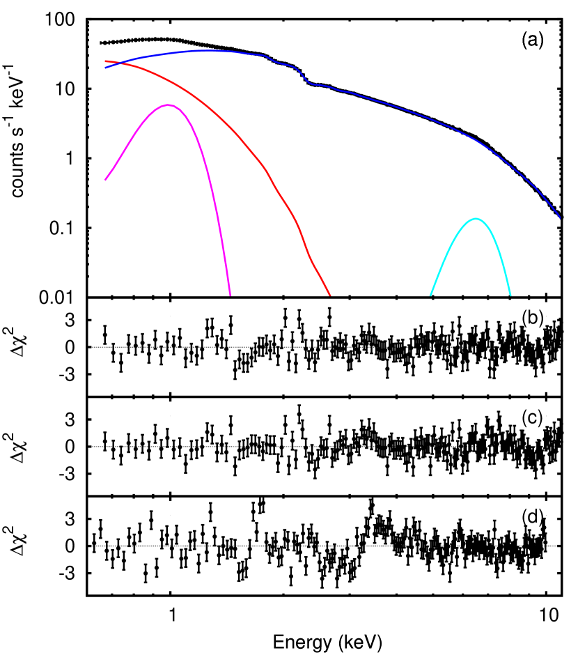
Figure 2: 0.6–11 keV spectrum observed by EPIC-pn during the persistent emission. The Comptonized component (blue), the accretion disc multi-temperature black-body (red) and the Gaussian features at 0.98 and 6.58 keV (magenta and light blue, respectively), used to model the spectrum according to Model A (see Table 1) are also plotted (panel a). Residuals of EPIC-pn data with respect to the best fitting Model A and B (see text and caption of Table 1) are plotted in panel (b) and (c), respectively. Residuals of the spectrum simultaneously observed by EPIC-MOS2 with respect to Model A (to which a couple of Gaussian absorption feature at $\sim 2$ keV were added) are plotted in panel (d).

Given the presence of small residuals at low $\lower 2.15277pt\hbox{$\;\buildrel<\over{\sim}\;$}2$ keV energies, and of a weak absorption feature at an energy close to the instrumental Si edge (1.84 keV), we also modelled the spectrum obtained after correcting the data with the task epfast. This tool is designed to reduce the possible effect of charge transfer inefficiency (CTI), and/or X-ray loading (XRL), on the spectra observed by the EPIC-pn in fast readout modes. It was calibrated to reduce residuals with respect to phenomenological models in the 1.5–3 keV, where the largest deviations are usually found (see the XMM-Newton calibration technical note, XMM-SOC-CAL-TN-0083, available at http://xmm.esac.esa.int/). However, the corrected spectrum resulted slightly more noisy than the unmodified one, and a further emission feature centred at 2.23(1) keV, close to the instrumental Au edge, should be added to the model; still the reduced chi squared of the fit (1.44 over 167 d.o.f.) was larger than the one obtained without correction, and for this reason we considered only the spectrum obtained without epfast correction. We note how the width and the normalisation of the feature at higher energy is left unchanged by epfast, while its centroid energy slightly increases with respect to the unmodified data, 6.66(7) keV. An increase of the iron line energy in epfast corrected data was already noted by Walton et al. (2012), who compared XMM-Newton and BeppoSAX spectra of XTE J1650–500, concluding how the unmodified EPIC-pn data possibly provided a better approximation of the true energy scale.

Reflection of the hard X-ray continuum above the accretion disc is the most convincing interpretation of the broad feature appearing at 6.58(7) keV, an energy compatible with K$\alpha$ transition of iron. We used the model reflionx (Ross & Fabian, 2005) to describe reflection arising from an optically thick ionised slab, illuminated by a $\Gamma=2$ power law spectrum. We convolved the reflection component with an exponential low-energy cutoff (expabs in XSpec), at an energy equal to the temperature of the soft seed photons of the nthcomp component, k$T_{\rm soft}$, to take into account the low energy rollover of the illuminating Comptonized spectrum. The reduced chi-squared obtained adding the reflection component to Model A, and removing the Gaussian feature at the energy of the iron K$\alpha$ transition, is 1.45 (250 over 172 d.o.f.). The ionisation parameter lies in the range $\log{\xi}=$2.7–2.8, compatible with the observed centroid energy of the iron line (see Table 1 of García et al., 2011). The addition of a Gaussian emission line centred at $\approx 1$ keV was still requested by the data, as the reflection model could not describe self-consistently the soft excess; removing the line from the model yielded in fact to a reduced chi-squared of $\simeq 4.5$, due to evident residuals at those energies. At the same time, the introduction of the reflection component made the soft thermal component not significantly detected anymore. However, the EPIC-pn response at energies $\lower 2.15277pt\hbox{$\;\buildrel<\over{\sim}\;$}2$ keV is clearly dominated by the Gaussian-shaped soft excess, found at a lower energy (0.78(5) keV) and with a larger equivalent width (153 eV) than the one obtained with model A, in which disc reflection was not self-consistently modelled. The non detection of the soft thermal component is then most probably due to correlation with the emission feature, whose energy is evaluated by this model to lie very close to the low energy end of the EPIC-pn energy band (0.6 keV). This is also confirmed by the detection of the disc thermal component in the spectrum obtained adding the RGS data-set, even when a reflection component is included in the model (see Sec. 3.3).

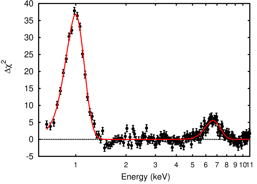
Figure 3: Residuals of the 0.6–11 keV EPIC-pn spectrum with respect to Model A (see text and Table 1), when the Gaussian emission features centred at 0.98 and 6.58 keV are removed from the model.

Table 1: Best fitting parameters of the X-ray spectrum of HETE J1900.1-2455. Columns labelled as Model A (EPn), TbNew(diskbb+nthcomp+gau₁+gau₂+gau₃), and Model B (EPn), TbNew(nthcomp+expabs*rdblur*reflionx+gau₂+gau₃), respectively, refer to the 0.6–11 keV spectrum observed by the EPIC-pn. Column labelled as Model A (RGS) refers to the modelling of the RGS1/2 spectra in the 0.33–2.07 keV. Column labelled as Model B (XMM-XTE), TbAbs*edge(nthcomp+expabs*rdblur*reflionx+gau₂+ gau₃+gau₄), reports the parameters obtained by modelling of the spectra obtained simultaneously by RGS1/2 (0.33–2.07 keV), EPIC-pn (0.6–11 keV), PCA (3–30 keV) and HEXTE (20–50 keV). Quoted fluxes are unabsorbed and evaluated in the 0.5–10 keV band for Model A (EPn) and B (EPn), in the 0.5–2 keV for Model A (RGS), and in the 0.5–50 keV band for Model B (XMM-XTE). The inner disc radius evaluated from the normalisation of the diskbb component, $R_{\rm disc}$, is given for an inclination of $30^{\circ}$. Uncertainties are evaluated at a $90$ per cent confidence level. Parameters held fixed in the fitting are reported without an uncertainty

	Model A (EPn)	Model B (EPn)	Model A (RGS)	Model B (XMM-XTE)
$N_{\rm H}$ ($10^{21}$ cm2)	1.3${}_{-0.6}^{+0.4}$	0.6(2)	1.02(5)	1.05(3)
$A_{\rm O}$	1	1	$2.11\pm 0.15$	$2.27\pm 0.11$
$kT_{\rm in}$ (keV)	0.21(1)	–	0.23${}_{-0.02}^{+0.03}$	0.202(7)
$R_{\rm disc}$ (d5 km)	31.1${}_{-8.5}^{+6.5}$	–	29.5${}_{-5.4}^{+6.7}$	33.4${}_{-2.2}^{+2.8}$
$\Gamma$	1.99(1)	1.979(7)	1.99	1.975(4)
$kT_{\rm soft}$	0.45(1)	0.458(4)	0.51${}_{-0.04}^{+0.06}$	0.446(5)
$kT_{\rm e}$	50	50	50	50
$N_{C}$ (10-2 cm${}^{-2}\>s^{-1}$)	6.7(2)	6.0(1)	6.51${}_{-0.6}^{+0.5}$	6.32(1)
$E_{1}$ (keV)	0.98(1)	0.78${}_{-0.06}^{+0.04}$	0.99(1)	0.94(1)
$\sigma_{1}$ (keV)	0.12(1)	0.24(3)	0.12(1)	0.13(1)
$N_{1}$ ($10^{-3}\>cm^{-2}\>s^{-1}$)	4.1$\pm$0.8	14${}_{-3}^{+5}$	3.8${}_{-0.8}^{+1.0}$	4.3(5)
EW1 (eV)	42	153	38	40
$E_{2}$ (keV)	6.58(7)	…	…	…
$\sigma_{2}$ (keV)	0.7(1)	…	…	…
$N_{2}$ ($10^{-3}\>cm^{-2}\>s^{-1}$)	0.6(1)	…	…	…
EW2 (eV)	135	…	…	…
$R_{\rm in}$ ($GM/c^{2}$)	…	23${}_{-7}^{+10}$	…	$25_{-11}^{+16}$
$R_{\rm out}$ ($GM/c^{2}$)	…	1000	…	1000
$\beta$	…	-3.8${}_{-5.2}^{+0.9}$	…	-3.7${}_{-2.5}^{+1.1}$
i (∘)	…	27$\pm$3	…	30.6${}_{-2.6}^{+3.7}$
$\log(\xi)$	…	2.76${}_{-0.04}^{+0.06}$	…	2.87${}_{-0.08}^{+0.16}$)
$R=F_{\rm refl}/F_{\rm nthc}$	…	0.10(1)	…	0.086(7)
$E_{3}$ (keV)	1.79(2)	1.82(2)	…	1.80(2)
$\sigma_{3}$ (keV)	0	0	…	0
$N_{3}$ ($10^{-4}\>cm^{-2}\>s^{-1}$)	-1.1(3)	-1.2(3)	…	-1.2(1)
$F$ ($10^{-10}$ erg cm-2 s-1)	7.3(2)	6.97(8)	2.46(2)	13.59(8)
$\chi^{2}_{r}$ (d.o.f.)	1.40(169)	1.36(169)	1.16(4201)	1.25(4460)

To investigate if the broadness of the emission features detected in the spectrum ($\sigma/E\approx 0.1$) could be explained in terms of relativistic effects expected to develop in the inner parts of the accretion disc, we convolved the reflection model with the rdblur kernel (Fabian et al., 1989). This model describes the relativistic effects due to the motion of plasma in a Keplerian accretion disc immersed in the gravitational well of the compact object, in terms of the inner and the outer radius of the disc, $R_{\rm in}$ and $R_{\rm out}$ (in units of the gravitational radius, $R_{\rm g}=GM/c^{2}$, where $M$ is the mass of the compact object), of the index of the assumed power-law dependence of the disc emissivity on the distance from the NS, $\beta$, and of the system inclination, $i$, respectively, by assuming the Schwarzschild metric. We held the value of the outer radius of the disc fixed to 1000 $R_{\rm g}$ as spectral fitting could not constrain it. Convolving the reflection model with such a component, the chi-squared of the fit decreased by $\Delta\chi^{2}=-20.9$, for the addition of three free parameters. In order to check the significance of such an improvement we used the method of posterior predictive $p$-values (Protassov et al., 2002). We created 1000 fake spectra using the best fit model without disc smearing, and fitted them with a model both including and excluding the blurring component. The probability that the chi-squared decrease observed in real data after introducing disk blurring is due to chance, is equal to the ratio between the number of cases in which a chi-squared decrease equal or larger than the one observed in real data was observed in fake spectra, and the number of trials. A chi-squared decrease equal or larger than that observed in real spectra was never obtained. We then estimated the probability that the improvement in spectrum description obtained by adding the disc smearing component to the model were due to chance as less than $10^{-3}$, concluding how this component was significant at a confidence level larger than 3-$\sigma$.The best-fitting parameters we obtained with this model, labelled as B, are given in the second column of Table 1, and the residuals with respect to the model are shown in panel (c) of Fig. 2.

3.2 Soft excess, MOS2 and RGS spectra

In the previous section, we described phenomenologically the strong excess appearing at $\approx 1$ keV in the EPIC-pn spectrum, by using a broad Gaussian emission line. Alternative modelling in terms of a bremsstrahlung continuum (bremss in XSpec) and an emission spectrum from hot diffuse gas (mekal), did not gave successful results in describing the excess, yielding a reduced chi-square of $\chi^{2}_{r}=5.7$ and 3.0, over 170 d.o.f., respectively. Several authors reported a similar excess at low energies in observations performed by the EPIC-pn in fast modes (see, e.g., Hiemstra et al., 2011; Walton et al., 2012). The amplitude of this excess seems to be correlated with the column density of the interstellar absorption towards the considered source, as it is expected in the case of an insufficient redistribution calibration (Guainazzi et al. 2012, XMM-SOC-CAL-TN-083). However, the column density of the interstellar absorption towards HETE J1900.1-2455 ($\simeq 10^{21}$ cm^-2) is lower than that affecting sources for which no significant excess was found (e.g., SAX J2103.5+4545, which has a $N_{\rm H}\simeq 6\times 10^{21}$ cm^-2), and thus no calibration induced excess should be expected if a correlation with the column density holds. Therefore, despite uncertainties in the instrument calibration may be responsible for at least part of this excess, we also explored plausible physical interpretations.

The centroid energy obtained with model A, 0.96(1) keV, is consistent with K$\alpha$ emission of Ne ix–x (0.92–1.02 keV), and the Fe-L$\alpha$ complex, which for $\log{\xi}$ ranging between 2 and 3 is made by transitions with energy between 0.8 and 1.2 keV (Kallman, 1995). Such transitions are produced by disc reflection, and are already included in the model reflionx; in particular the prominence of the Fe-L$\alpha$ line is expected to grow when the reflecting slab is iron-rich (Ross & Fabian, 2005; Fabian et al., 2009). Removing the Gaussian feature and letting the iron abundance of the reflection component of Model B free to vary, we obtained a best-fit abundance of 2.00(5) with respect to Solar values, while other parameters of the reflecting medium were compatible with those listed in Table 1 ($\beta\leq 4.6$, $R_{\rm in}=27^{+3}_{-5}\>R_{\rm g}$, $i=29(1)^{\circ}$, $\log{\xi}=2.70(2)$, $R=F_{\rm refl}/F_{\rm nthc}=0.10(1)$; the reflection fraction $R$ is evaluated as the ratio between the unabsorbed fluxes in the reflected and Comptonized component, in the 0.5–10 keV band). However, the reduced chi-square of the fit, 2.34 over 169 degrees of freedom, is much larger with respect to Model B as residuals appeared at energies below 2 keV even after the addition of a diskbb component to the model. We also tried to fit the spectrum obtained discarding energies above 5 keV; a successful modelling is found with similar parameters than before, but this time with a larger reflection fraction, $R=0.27(2)$. The large flux in the $\approx 1$ keV feature with respect to the iron line is then the most probable reason for the non-achievement of a simultaneous modelling of the hard and soft part of EPIC-pn spectrum in terms of the same reflecting environment. At the same time, we could not model successfully the whole EPIC-pn energy band even by using two reflection components.

We then explored if part of the excess could be interpreted to an overabundance of Ne in the same reflector originating the Fe K$\alpha$ line. Unfortunately, abundances of metals other than Fe cannot be adjusted in reflionx. We then added a line blurred by the same rdblur kernel used to convolve the reflection component, to the previous model. A line centred at 0.95(1) keV improved the modelling, but the chi-squared we obtained, 1.45 over 167 d.o.f., was still larger than that obtained simply modelling the feature with a Gaussian (1.36 over 169 d.o.f., see Model B listed in Table 1), indicating how such a modelling was not completely satisfactory.

In order to verify the origin of such an excess, we considered spectra observed by other instruments on-board XMM-Newton. The MOS2 spectrum is much more noisy with respect to EPIC-pn, probably because of a more uncertain energy calibration when operated in timing mode; two additional absorption features were added in the Au K-edge region around 2 keV, but still the final reduced chi-square was far from being acceptable (2.62 over 166 d.o.f.; see bottom panel of Fig. 2 for residuals with respect to Model A). Nevertheless, we detected a Gaussian-shaped feature with parameters entirely compatible with those found by EPIC-pn ($E_{1}=0.97(1)$ keV, $\sigma_{1}=0.12(2)$ keV, $N_{1}=4.7(2)\times 10^{-3}$ cm^-2 s^-1, EW${}_{1}=45(1)$ eV)

To model RGS spectra, we considered only first order spectra in 0.33–2.07 keV band, since the second order added no information. We modelled the continuum as in model A, with a multicoloured disc black-body and a Comptonized component; given the limited bandwidth covered by the RGS, we fixed the value of the asymptotic power law index of the Comptonized component to the value indicated by the EPIC-pn analysis (see leftmost column of Table 1). We modelled interstellar absorption with TbNew, and let a relative normalisation constant between the two RGS spectra free to vary. As residuals appeared around the O i K edge at (0.54 keV), and close to the O i 1s–2p transition (0.5275 keV), we let the abundance of O as a free parameter, obtaining a best-fit value of $A_{\rm O}=2.11\pm 0.15$ with respect to a H column density of $N_{\rm H}=1.0(5)\times 10^{21}$ cm². We found an excess around $\sim 1$ keV in RGS data as well (see Fig. 4, where the residuals obtained removing the lines from the best-fitting models, are shown); by modelling it with a Gaussian feature, parameters entirely compatible with those obtained modelling the EPIC-pn data with model A, were found. Including the Gaussian feature the chi-squared of the fit decreased by $\Delta\chi^{2}=-181.2$. To check the significance of this excess, we applied the same method of posterior predictive $p$-values described in the previous section. This yielded a probability of $p\leq 10^{-3}$ of the observed improvement being due to chance. The best fitting values of the parameters are listed in the column labelled as Model A (RGS) of Table 1. A possible correlation with the composition of the medium yielding interstellar absorption could be excluded, as even varying the abundances of the atomic species with edges falling in the considered energy band, a chi-squared similar to that obtained with the Gaussian feature could not be obtained; at the same time, contribution from absorption of O viii, could be excluded as the fit with an edge fixed at 0.87 keV did not determine a fit of a comparable quality.

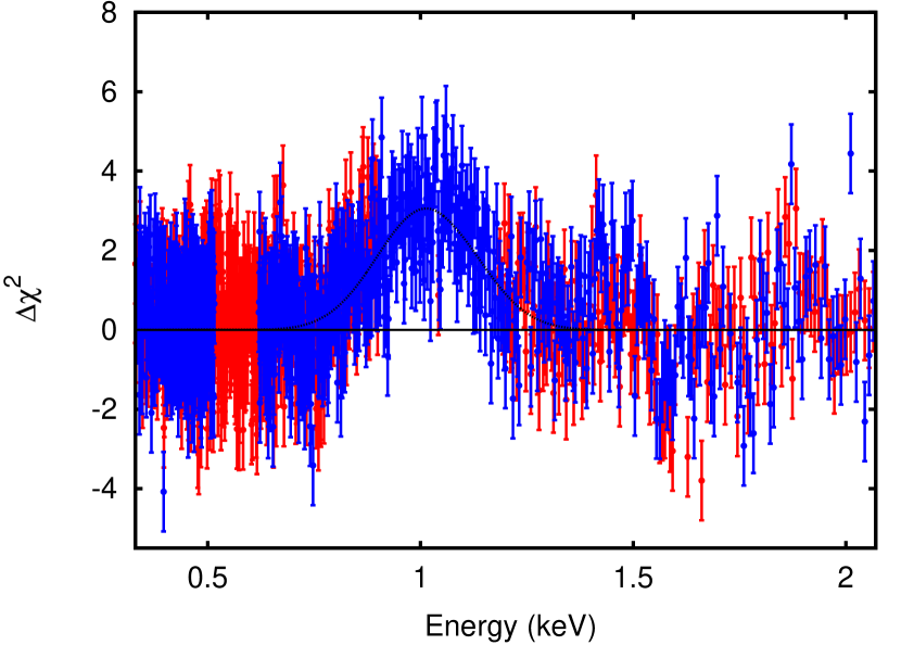
Figure 4: Residuals of the 0.33–2.07 keV spectra observed by the RGS1 (red points) and RGS2 (blue points) with respect to Model A (RGS; see caption of Table 1 and Sec. 3.2), when the Gaussian emission feature centred at 0.99 keV is removed from the model.

3.3 Simultaneous RXTE - XMM-Newton spectrum

Analysis of the observation performed by RXTE simultaneously to XMM-Newton allows to constrain on a broader energy band the X-ray spectrum of HETE J1900.1-2455. By using the same bands defined by Watts et al. (2009) we obtained values of the soft and hard colour of 1.1 and 1.0, respectively. Comparing these values with those plotted in Fig. 4 of Watts et al. (2009), we conclude that during this observation HETE J1900.1-2455 was in the softer end of the hard island state.

We fitted the spectra observed by PCA (3–30 keV) and HEXTE (20–50 keV) on-board RXTE simultaneously to those obtained by RGS1/2 (0.33-2.07 keV) and by EPIC-pn (0.6–11 keV), fixing the normalisation constant of the EPIC-pn spectrum to one, and letting a relative normalisation constant free to vary for the other spectra. We obtained a reduced chi-squared of 1.24 over 4458 degrees of freedom by using Model B (see Table 1), and letting the abundance of O in the interstellar medium as a variable parameter. Unlike the case described in Section 3.1, we significantly detected a diskbb component even with a reflection component included in the model, as its addition decreased the chi-squared by $\Delta\chi^{2}=-432$ for two d.o.f. more. The Gaussian-shaped feature at $\sim 1$ keV was described by parameters compatible with those found when modelling both EPIC-pn and RGS data with model A. The detection of a disc reflection component was significant also in the broad-band spectrum, since removing it from the model yielded a chi-squared increase of $\Delta\chi^{2}=314$ for five d.o.f. more. The parameters of disc reflection are compatible with those indicated by the analysis of EPIC-pn data alone, indicating an inclination of $i=(30.6^{+3.7}_{-2.6})^{\circ}$ and an inner disk radius of $R_{\rm in}=25_{-11}^{+16}$ R_g. The best-fitting parameters are shown in the rightmost columns Table 1, the unfolded spectrum is plotted in the upper panel of Fig. 5, and residuals with respect to the best-fit model shown in the lower panel.

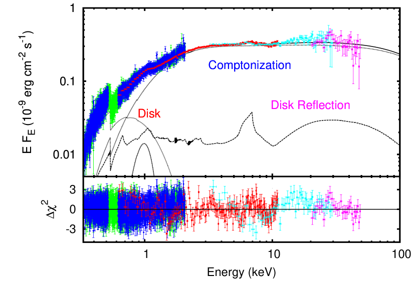
Figure 5: 0.33–50 keV unfolded spectrum of HETE J1900.1-2455 obtained fitting simultaneously spectra from RGS1/2 (0.33–2.07 keV, blue and green points, respectively), EPIC-pn (0.6–11 keV, red), PCA (3–30 keV, cyan) and HEXTE (20–50 keV, magenta) and considering Model B (see Table 1), whose component are also over-plotted (top panel). Residuals with respect to Model B (bottom panel).

To check if a slightly mis-calibrated response of the EPIC-pn at low energies could affect model parameters, and in particular those describing the reflection component, we also performed spectral fitting after removing EPIC-pn data below 2 keV. The best-fitting model had a reduced chi-squared of 1.22 (over 4427 d.o.f.) and no significant difference with respect to the parameters listed in the rightmost column of Table 1 was found. It is worth noting that in this case, the excess at $\approx 1$ keV was satisfactorily modelled by a reflection model with a Fe abundance of $2.0_{-0.20}^{+0.06}$ times the Solar value, without the need of an additional Gaussian feature. At the same time, given the slight mismatch between the PCA and the EPIC-pn residuals (see bottom panel of Fig. 5), we removed the PCA data below 8 keV, but still no significant variations were found in the model parameters.

4 Temporal analysis

In order to search the EPIC pn time series for a periodicity at the 377.3 Hz spin frequency of HETE J1900.1-2455, we first reported the photon arrival times to the Solar system barycentre using the source coordinates of the optical counterpart estimated by Fox (2005). Since the pulse amplitude of AMSPs usually decreases below 2 keV (Patruno et al., 2009; Papitto et al., 2010), compatible with the increasing contribution of the accretion disc to the overall flux, we restricted our analysis to the 2–11 keV energy band. We corrected time delays induced by the orbital motion of the source in the binary system using ephemeris determined by Patruno (2012), who derived a timing solution valid over a time interval of 2.6 yr (MJD 53539–54499) based on RXTE/PCA data. To ascertain whether the uncertainties on this set of parameters are small enough not to affect coherence of the signal over the EPIC pn exposure, we considered the relations given by Caliandro et al. (2012), who estimated the reduction of the power obtained with a Fourier transform of a coherent signal, $\epsilon^{2}$, as a function of the difference between actual orbital parameters and the estimates used to correct photon arrival times. We evaluated the relations they derived (see their Eq. 52, 64, 68, 72) for the orbital and spin parameters of HETE J1900.1-2455 and a signal power reduction of $\epsilon^{2}=0.8$; to produce a similar power decrease, the estimates of semi-major axis of the NS orbit, eccentricity, epoch of zero mean anomaly, and orbital period used in arrival time corrections should differ by $\delta x=1.7\times 10^{-3}$ lt-s, $\delta e=0.04$, $\delta T^{*}=30$ s, $\delta P_{\rm orb}=2.7$ s, from the actual values, respectively. All but $\delta T^{*}$ are more than two orders of magnitude larger than uncertainties quoted by both Patruno (2012) and Kaaret et al. (2006), indicating how available estimates were accurate enough not to induce loss of signal power. The uncertainty on the epoch of zero mean anomaly was evaluated by propagating the uncertainty on the estimate evaluated at the reference epoch of the timing solution given by Patruno (2012) ($t_{0}=\rm{MJD}\>53538.76$, Patruno, priv. comm.), through the $\Delta t=6.25$ yr elapsed until the XMM-Newton observation (see, e.g. Papitto et al., 2005)

$$\sigma_{T^{*}}(t_{\rm EPN})= \bigg{\{}[\sigma_{T^{*}}(t_{0})]^{2}+\left[\sigma_{P_{orb}}\frac{\Delta t}{P_{\rm orb}}\right]^{2}+$$ (1)

$$\left[\frac{1}{2}P_{\rm orb}\dot{P}_{orb}\left(\frac{\Delta t}{P_{\rm orb}}\right)^{2}\right]^{2}\bigg{\}}^{1/2}=464s,$$

where $P_{\rm orb}=4995.2630(5)$ s is the orbital period, $\sigma_{T^{*}}=0.8$ s and $\sigma_{P_{orb}}=5\times 10^{-4}$ s are the uncertainties on the epoch of zero mean anomaly and orbital period, respectively, and $\dot{P}_{orb}<1.2\times 10^{-10}$ is the upper limit on the orbital period derivative at 95 per cent confidence level (Patruno, 2012). As long as such loose upper limit on $\dot{P}_{orb}$ is considered, $\sigma_{T^{*}}(t_{\rm EPN})\simeq 15\>\delta T^{*}$, and $n_{T^{*}}=90$ corrections with values of $T^{*}$ differing by $\delta T^{*}$, should have been performed to cover all the possible value of $T^{*}$, ranging from $T^{*}(t_{\rm EPN})-3\sigma_{T^{*}}(t_{\rm EPN})$ to $T^{*}(t_{\rm EPN})+3\sigma_{T^{*}}(t_{\rm EPN})$. However, the orbital period derivative measured from SAX J1808.4–3658 (Hartman et al., 2008; Di Salvo et al., 2008; Hartman et al., 2009; Burderi et al., 2009; Patruno et al., 2012), a source with orbital parameters similar to those of HETE J1900.1-2455, is $\sim 25$ times smaller than the upper limit given by Patruno (2012) for HETE J1900.1-2455. The value measured for SAX J1808.4–3658 is already so large that largely non conservative scenarios of mass transfer should be invoked to explain it (Di Salvo et al., 2008; Burderi et al., 2009). Consider an orbital period derivative equal to the value measured for SAX J1808.4–3658, we obtained $\sigma_{T^{*}}(t_{\rm EPN})=23.9$ s; only $n^{\prime}_{T*}=6\>\sigma_{T^{*}}(t_{\rm EPN})/\delta T^{*}\simeq 5$ trials were then needed to cover possible values of $T^{*}(t_{\rm EPN})$, when a plausible value of the orbital period derivative of HETE J1900.1-2455 was considered.

To determine over which frequency range a meaningful search for a signal at the spin period of HETE J1900.1-2455 should have been performed, we evaluated the spin frequency variation $\Delta\nu$ driven by the accretion between 2005 and 2012. Assuming the base level spin frequency derivative estimated by Patruno (2012), $\dot{\nu}=4.2(1)\times 10^{-14}$ Hz s^-1, compatible with the torque expected to be imparted by mass accretion at a rate of few $\times 10^{-10}$ M_⊙ yr^-1 onto a NS with magnetic field $\simeq 10^{8}$ G, we obtained $\Delta\nu=8.3(2)\times 10^{-6}$ Hz. Since the frequency Fourier resolution of a power spectrum produced over the 60 ks EPIC pn time series is $\delta\nu_{F}=1/T_{\rm obs}=1.67\times 10^{-5}$ Hz, one frequency bin contains both the value of the spin frequency in 2005 ($377.29617188$ Hz, Patruno, priv. comm.) and the one expected in 2012 ($377.2961802(2)$ Hz). We did not detect any significant signal in power spectra of the time series corrected with the $n^{\prime}_{T^{*}}=5$ plausible values of $T^{*}$, inspecting a single frequency bin centred at 377.2961735 Hz, of width equal to $\delta\nu_{F}$. The maximum Leahy power we obtained is $P_{\rm max}=4.7$, lower than the 3-$\sigma$ confidence level threshold (van der Klis, 1989; Vaughan et al., 1994)

$$P_{3\sigma}(n_{tot}=5)=2\ln{(n_{tot})+2\ln{(p^{-1})}}=15.0.$$ (2)

This threshold is obtained by evaluating the power level that has a probability lower than $p=2.7\times 10^{-3}$ of being exceeded by noise powers distributed as a $\chi^{2}$ with two degrees of freedom, taking into account the five trials performed ($n^{\prime}_{T^{*}}=5$, $n_{\nu}=1$). We took into account the effect of noise-signal interactions due to the fact that the total power in a frequency bin is the square of the sum of noise and signal Fourier amplitude, each of which is a complex number (Groth, 1975). To this aim we used the routine given by Vaughan et al. 1994; the maximum observed power translates into an upper limit on the signal power of $P_{\rm UL}=23.2$, at $3\sigma$ confidence level. Considering that the total number of photons in the time series is $N_{\gamma}=3.96\times 10^{6}$, and that the average power reduction due to frequency and $T^{*}$ binning is $\xi_{\nu}=0.773$ (Vaughan et al., 1994) and $\xi_{T^{*}}\simeq 1-\epsilon^{2}/2=0.9$, respectively, the 3-$\sigma$ upper limit on the pulse amplitude is (Vaughan et al., 1994)

$$A_{UL}=\left\{\frac{2}{\xi_{\nu}\xi_{T^{*}}}\frac{P_{\rm UL}}{N_{\gamma}}\left[\mbox{sinc}\left({\frac{\pi}{2}\frac{\nu}{\nu_{Ny}}}\right)\right]^{-1}\right\}^{1/2}=4\times 10^{-3}.$$ (3)

Here, $\mbox{sinc}(x)=\sin(x)/x$, and the Nyquist frequency is $\nu_{\rm Ny}=1/(2\>n_{\rm bin}\>t_{res})=2117$ Hz, as the time resolution of the series is $t_{res}=2.952\times 10^{-5}$ s and we set $n_{\rm bin}=16$.

Even by extending the parameter space over which we searched for a signal, inspecting all the values of T^∗ compatible with the loose available upper limit on the orbital period derivative ($n^{\prime}_{T^{*}}=90$, $n_{\nu}=1$, $P_{3\sigma}(n_{tot}=90)=20.8$), and the two nearest Fourier independent frequencies ($n^{\prime}_{T^{*}}=90$, $n_{\nu}=3$, $P_{3\sigma}(n_{tot}=270)=23.0$), no detection was achieved ($P_{\rm max}=11.0$). As some of the detections claimed by Patruno (2012) were achieved on short time intervals, we performed a pulsation search over $n_{s}=120$ data segments as short as 500 s ($n^{\prime}_{T^{*}}=5$, $n_{\nu}=1$, $P_{3\sigma}(n_{tot}=600)=24.6$), but still found none significant at a 3$\sigma$ confidence level ($P_{\rm max}=19.7$).

To study the aperiodic properties of the source, we averaged 1940 power density spectra produced over $\simeq$31 s long intervals, retaining photons in the full 0.3–11 keV bandwidth, and re-binning the resulting spectrum by a factor 1.03. Four Lorentzians components were used to model the power spectrum obtained after the subtraction of a white noise level of 1.992(2) Hz^-1 (see Fig. 6): two flat-top noise components (i.e. centred at zero frequency), with width $W_{1}=0.80(1)$ and $W_{2}=47(7)$ Hz, and two narrower Lorentzians centred at $\nu_{3}=1.98(2)$ and $\nu_{4}=2.6(2)$ Hz, with width $W_{3}=0.4(1)$ and $W_{4}=3.6(3)$ Hz, labelled as $L_{1}$, $L_{2}$, $L_{3}$ and $L_{4}$, respectively. A similar decomposition is remarkably similar to that shown by atoll sources in the hard state (Olive et al., 1998), and other AMSPs (van Straaten et al., 2005). In particular, the frequency and quality factor (defined as $\nu/W$) of features we denoted as $L_{3}$ and $L_{4}$ are similar to those of the quasi periodical oscillations identified by van Straaten et al. (2005) as $L_{\rm LF}$ and $L_{h}$, in low luminosity, non-pulsing atolls, such as 1E 1724–3045 and GS 1826–24. High frequency quasi periodical oscillations were also searched for, by averaging 16 s long intervals, but none was found.

Figure 6: Power spectrum obtained by averaging 1940 intervals, each $\simeq$31 s long, and re-binning the resulting spectrum with a factor 1.03. A white noise level of 1.992(2) was subtracted. The solid line is the best-fit model composed of four Lorentzian components, which are also shown as dotted lines (top panel). Residuals in units of $\sigma$ with respect to the best-fit model (bottom panel).

5 X-ray burst

A type-I X-ray burst was observed during XMM-Newton exposure (see inset of Fig. 1 for the 0.6–11 keV light curve), starting on MJD 55823.69344. During first $\sim 10$ s since the burst onset, EPIC-pn count-rate saturated at a level of $\sim$ 1900 s^-1 due to telemetry limitation, and the light curve cannot be considered representative of the true burst light curve shape (see top panel of Fig. 7). Presumably for the same reason, data were not acquired during intervals 14 – 24 and 34 – 44 s, since the burst start. At later times since the burst onset, the profile could be modelled with an exponential decay with a time constant of $\tau=46(1)$ s. This is significantly longer than the length of the majority of bursts observed by RXTE and HETE (Suzuki et al., 2007; Galloway et al., 2008; Watts et al., 2009), except for the burst labelled as B1 in Fig. 2 of Watts et al. 2009, and which also took place where the source was in the hard state. However, there does not seem to be a clear correlation of burst duration with the position of the source in a colour-colour diagram; the position of the source during the observation considered here is in fact much closer to that shown by the source before shorter bursts (e.g. burst B4 in Fig. 4 of Watts et al. 2009), than at the onset of the other long burst detected.

We searched for burst oscillations over 4 s intervals of EPIC-pn data; we inspected frequencies ranging from 374 to 378 Hz, for a total of 16 trials in every interval, in order to cover the interval over which the frequency of burst oscillations discovered by Watts et al. (2009) was observed to vary. We found a barely significant signal at a frequency of 377.04(25) Hz with a Leahy power of 21.6, in the interval starting 24 s after the burst onset. Such a power is larger than the 3$\sigma$ threshold for a single interval (17.2), but reduces to a significance of 2.1$\sigma$ if the number of intervals considered to analyse the burst (100) is taken into account; we cannot therefore exclude it represents a statistical fluctuation. The folded profile is shown in the inset of Fig. 7. If the oscillations were effectively present, this would be the first time they were observed in the hard state, since oscillations reported by Watts et al. (2009) were found in a short duration burst, ignited when the source was in a soft state. We note that before the interval where the marginal detection was achieved, sensitivity to pulsed signals was severely reduced due to telemetry overload.

For the same reason, time-resolved spectroscopy of the burst could be meaningfully performed only after $\sim 25$ s since the burst onset. No background was subtracted, and the best-fit Model A (see leftmost column of Table 1) was used to model persistent emission, letting only the absorption column free to vary. Spectra in the 0.6–11 keV energy band were satisfactorily fit by an absorbed black-body, with a temperature decreasing from 1.6(1) to 0.9(1) keV at the end of the burst, and an apparent radius roughly constant around a value of $\sim 6$ d₅ km. The value of the absorption column density we found, $N_{\rm H}=(0.99\pm 0.15)\times 10^{21}$ cm^-2 is compatible with estimates indicated by analysis of persistent emission (see Table 1).

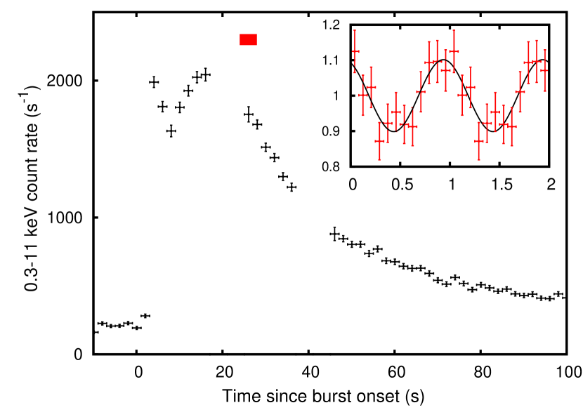
Figure 7: 0.6–11 keV light curve of the burst observed by EPIC-pn on-board XMM-Newton. Time is shown in seconds since the burst onset. The horizontal bar indicates the time interval during which a signal is barely detected at a Leahy power of 21.6. The inset shows the profile obtained by folding data obtained during such interval, around the frequency, 377.04(25) Hz.

6 Discussion and conclusion

LMXB hosting a NS are usually classified in Z and atoll sources, based on the track followed in a colour-colour diagram and the aperiodic time variability (Hasinger & van der Klis, 1989), with atolls emitting a luminosity $\lower 2.15277pt\hbox{$\;\buildrel<\over{\sim}\;$}0.5$ L_Edd, and showing a harder spectrum, on average. Similar to other AMSP, HETE J1900.1-2455 behaves as a typical atoll source, spending most of the time in the hard island state (Watts et al., 2009). Also the observations considered here caught the source in such state, while emitting a 0.33–50 keV unabsorbed luminosity of $4.07(3)\times 10^{36}$ erg s^-1; roughly $90$ per cent of the X-ray observed in such band is described by a $\Gamma\simeq 2$ hard component, with no cut-off significantly detected in our data. To physically model such a component we used Comptonization of soft, $kT_{\rm soft}\simeq 0.45$ keV, photons in a medium with an electron temperature fixed to 100 keV. The slope of such hard component and the assumed electron temperature indicate an optical depth, $\tau\simeq 1$ (Zdziarski et al., 1996; Życki et al., 1999). A similar Comptonized component was used by Falanga et al. (2007) to model the 2–300 keV spectrum observed by RXTE and INTEGRAL during observations performed in 2005, and is invariably found to dominate the X-ray spectrum of AMSP (Poutanen, 2006). Considering also the energy-dependent properties of pulse profiles, Gierliński et al. (2002) interpreted this component as originated in the accretion columns, where mass is channelled by the magnetic field and heated by the interaction with radiation coming from the NS surface. However, the non detection of pulsations casts doubts on the presence of accretion columns during the observation of HETE J1900.1-2455 presented here.

Two broad emission features centred at energies 0.98(1) and 6.58(7) keV were detected in EPIC-pn spectrum. The energy of the latter is compatible with K$\alpha$ transition of Fe xxiii–xxv (6.6–6.7 keV, see, e.g., Kallman et al., 2004); such detection confirms the results previously obtained by Cackett et al. (2010) with a Suzaku observation, and by Falanga et al. (2007), even if at a much lower spectral resolution. Origin of the $\approx 1$ keV feature is instead less clear. Calibration uncertainties of the EPIC-pn spectra taken in timing mode were often invoked to explain appearance of strong features at energies $\lower 2.15277pt\hbox{$\;\buildrel<\over{\sim}\;$}1$ keV; however, the presence of a similar line-shaped residual also in spectra observed by EPIC-MOS2 and RGS strongly suggests a physical origin. Both the features have a broadness $\sigma/E\simeq 0.1$, compatible with a similar mechanism determining their shape. The easiest interpretation of such width is in terms of reflection of hard X-ray photons in the accretion disc, where the strong velocity field broadens discrete features, and relativistic effects distort and smear their shape, shifting them towards lower energies. In the case of the observations analysed here, a mildly ionised $\xi\simeq 750$ erg cm s^-1 disc reflection component, broadened by motion in an accretion disc and representing $10$ per cent of the overall flux, successfully models the iron line and improves description of the spectral continuum. However, a self-consistent modelling of the two discrete features, could not be obtained, as far as the EPIC-pn data below 2 keV are considered. Strong emission features at energies similar than those found here were recently reported thanks to XMM-Newton spectra of a couple of narrow-line Seyfert 1 galaxies, and interpreted in terms of emission lines due to Fe K$\alpha$ and Fe L$\alpha$ transitions taking place as the accretion disc reflects hard illuminating emission (Fabian et al., 2009; Ponti et al., 2010; Zoghbi et al., 2010; Fabian et al., 2012). Despite the ratio between the photon fluxes in the two features observed by EPIC-pn ($=6.8\pm 1.7$) is less extreme than those they reported ($\lower 2.15277pt\hbox{$\;\buildrel>\over{\sim}\;$}20$), it is still too large to be described by a single reflection environment like that we considered. A lower flux ratio is in fact expected when the illuminating spectrum becomes softer than $\Gamma\lower 2.15277pt\hbox{$\;\buildrel<\over{\sim}\;$}2$ at a given flux, and iron is less ionised (Ross & Fabian, 2005). However, excluding from the fit EPIC-pn data below 2 keV and modelling low energies with RGS data alone, we could find a self-consistent modelling of the two features in the same reflecting environment, with an iron abundance $\approx 2$ times larger than the Solar value. Another, not necessarily alternative interpretation of the excess is in terms of K$\alpha$ transition of overabundant helium-like Ne; though, it was not possible to vary the abundance of this element in the reflection model, and simply adding a blurred feature at the relevant energy did not result in a completely satisfactory description. The failure in deriving a simultaneous description of the feature detected by EPIC-pn possibly follows from superimposition of different transitions not completely taken into account by the reflection model used, different abundances of ionised elements, or because of residual calibration uncertainties. The satisfactory modelling of the two features by a reflection component with overabundant iron, obtained when EPIC-pn data at low energies are discarded, favours the latter hypothesis. In any case, the simultaneous detection of such feature from different instruments makes it a very promising additional probe of the accretion flow to LMXB hosting NS, the nature of which will be firmly assessed by future observations.

Fitting the smeared reflected component with the rdblur kernel of Fabian et al. (1989), we estimated the inclination, the emissivity, the inner radius of the disc, $i=(30.6^{+3.7}_{-2.6})^{\circ}$, $\beta\simeq-3.7^{+1.1}_{-2.5}$, $R_{\rm in}\simeq 25^{+16}_{-11}\>R_{g}$, respectively. From Doppler tomography of a broad H$\alpha$ line assumed to originate in the accretion disc, Elebert et al. (2008) estimated the inclination of the system to be $i\lower 2.15277pt\hbox{$\;\buildrel<\over{\sim}\;$}20^{\circ}$ for a 1.4 $M_{\odot}$, a value not far from that reported here. Our estimate of the inner disc radius is compatible with the value of $14(1)$ R_g found by Cackett et al. (2010, for a rather low inclination of 4^∘), who modelled a Suzaku spectrum of this source taken when its 0.5–25 keV luminosity was $\simeq 5\times 10^{35}$ erg s^-1 (roughly a factor three times lower than during the observations presented here) by adding a reflection component to a $\Gamma\simeq 2.2$ power law. At a distance of $\approx 25\>R_{g}$ from the compact object, relativistic effects are small and the line shape we observed is rather symmetric. However, alternative interpretations proposed to explain broad symmetric iron lines, such as Compton broadening in a hot corona, are not compatible with what observed in the broadband spectral decomposition. An optically thin, $\tau\sim 1$ corona causes an average photon energy shift of $\Delta\epsilon/\epsilon=(4kT_{e}-\epsilon)/m_{e}c^{2}$ (Rybicki & Lightman, 1979); to produce the observed line width of $0.7(1)$ keV, the electrons in the Comptonizing cloud should have a temperature of $\simeq 15$ keV and a similar component was not observed in the spectrum. The value estimated for the inner disc radius translates into a value of 52${}_{-23}^{+33}$ km, for a 1.4 $M_{\odot}$ NS. Despite the large uncertainty affecting this estimate ($R_{\rm in}>12$ km at 99 per cent confidence level), the shape of reflected spectrum indicates that the accretion disc is truncated. A similar size of the inner rim of the disc is suggested also by the $kT_{\rm in}\simeq 0.2$ keV thermal component detected at low energies; if modelled with an accretion disc model, its normalisation indicates an apparent inner disc radius $\simeq 30$ d₅ km (for $i=30^{\circ}$). The actual inner radius of the disc can be larger up to a factor of two than this estimate, when colour corrections are considered (Merloni et al., 2000) and torque is assumed to be retained through the transition region from the optically thick disc to the inner hot flow (Gierliński et al., 1999). At the same time, considering the luminosity of the photo-ionising Comptonized component ($L_{\rm irr}\simeq 3.5\times 10^{36}$ d${}_{5}^{2}$ erg s^-1), the ionisation parameter of the observed reflected component (${\xi}=L_{\rm irr}/n_{\rm H}\rho^{2}\simeq 750$ erg cm s^-1) is expected to be produced at a distance $\rho\simeq 30$ km from the source of illuminating photons, for a hydrogen density of $5\times 10^{20}$ cm^-3, a value appropriate for a Shakura Sunyaev disc around an accreting NS (see, e.g., Ross & Fabian, 2007). Further, for a 10 km NS and a system inclination of $30^{\circ}$, the observed ratio between the reflected and illuminating component ($\simeq 0.1$, corresponding to a reflection amplitude $\Omega/2\pi\simeq 0.13$) indicates an inner disc radius $\lower 2.15277pt\hbox{$\;\buildrel>\over{\sim}\;$}50$ km (Gierliński & Poutanen, 2005, who calculated the reflection amplitude as a function of the inner disc radius in the case of a small illuminating spot at the rotational pole of the NS; a more extended source of illuminating photons produces a larger reflection amplitude at a fixed disc radius).

The main peculiarity of HETE J1900.1-2455 is coherent pulsations intermittence, whose causes are not yet fully understood. Cumming (2008) proposed that intermittence is caused by a screening of the magnetosphere and burial of the magnetic field under the NS surface. On the other hand, Romanova et al. (2008) and Lamb et al. (2009), while involving the presence of a magnetosphere, explained intermittence in terms of penetration of in-falling matter through the magnetic field lines, and of movements of a hot spot located close to the spin axis of the NS, respectively, depending on variations of the mass accretion rate. Alternative scenarios proposed to explain the paucity of pulsars among LMXB, and possibly related to pulse intermittence, include scattering in a hot, relatively optically thick cloud surrounding the NS (Titarchuk et al., 2002), and reduction of pulse amplitude due to gravitational light bending (Özel, 2009). However, considering how a Comptonized component produced in an optically thin, $\tau\approx 1$, corona was observed regardless of pulse detection, and how the compactness of the NS hardly varies on timescales of few years, these two latter interpretations do not reproduce easily the behaviour observed from HETE J1900.1-2455. The evidences we obtained from spectral analysis of an accretion disc truncated quite far from the NS have to be discussed in view of the time variability shown by the source. No pulsations were detected during the persistent emission, with a very low upper limit of 0.4 per cent, at 3 $\sigma$ confidence level, on the 2–11 keV pulsed fractional amplitude. Such a limit is of the same order of the weaker pulsations detected by Patruno (2012). As already suggested by Galloway et al. (2008), this source could persistently show pulsations at a very low, $\lower 2.15277pt\hbox{$\;\buildrel<\over{\sim}\;$}0.1$ per cent, amplitude, beyond the detection sensitivity of current instruments. The inner disc radius derived by spectral modelling of the reflection component is compatible with models in which a magnetosphere is able to truncate the optically thick disc, and coherent oscillations are reduced in amplitude by geometrical effects (Lamb et al., 2009) and/or by weak channelling of accreting matter, if any (Romanova et al., 2008). However, the tight upper limit on pulse amplitude and the absence of a clear relation between appearance of pulses and variations of the mass accretion rate, do not necessarily favour them. On the other hand, spectral and aperiodic timing properties of this source are entirely indistinguishable to that of (assumed) non pulsing atolls in the hard state, suggesting how the accretion flow to HETE J1900.1-2455 is probably not channelled by a magnetosphere. This would keep open the possibility of a buried magnetic field (Cumming, 2008). In such a scenario, the optically thick flow in a geometrically thin accretion disc would be replaced by a inner optically thin hot flow, rather than by a magnetospheric flow. This fits into the truncated disc scenario explaining hard states shown by both accreting black holes and neutron stars (see, e.g., Done et al., 2007, for a review). Similar estimates of the inner disc radius were indeed obtained from iron line modelling of non-pulsing atolls in the hard state (e.g., the cases of 4U 1705–44 and MXB 1728-34; D’Aì et al., 2010; Egron et al., 2011, 2012). It remains an open question whether the accretion disc flow is truncated by a similar mechanism, connected to the overall evolution of the accretion disc rather than to the NS magnetic field, even when a magnetosphere is certainly present (i.e., when pulsations are detected). Long observations of AMSPs performed while they show pulsations, and aimed at a detailed modelling of broad emission features, will be crucial to this end.

During the XMM-Newton observation a type-I X-ray burst was detected. Because of telemetry overflow, we could not determine the peak burst luminosity, nor if a photospheric radius expansion took place. We barely detected a signal at a frequency of 377.04(25) Hz during a 4 s interval, 24 s after the burst onset; however, the observed power is low, and the signal is significant only if the number of burst intervals inspected is not taken into account. Burst oscillations from this source were already found by Watts et al. (2009) during a short burst ($\tau=7$–$8$ s). The burst during which they detected pulsations ignited when the source was in the soft (banana) state, with a a 2–16 keV flux of $\approx 63$ mCrab as observed by RXTE/PCA, which is to date the highest persistent flux at which bursts have been detected in this source. Oscillations were detected during the initial stages of the burst decay, at a frequency $\sim 1$ Hz below the spin frequency of the source, drifting towards this value as the burst evolved. On the other hand, the 46 s time decay of the burst reported here, the persistent source flux (24 mCrab in the 2–16 keV range) and the hard spectral state are not easily reconciled with the general picture of the non-pulsing LMXBs and intermittent pulsars, which preferably show oscillations during short bursts ignited when the source is in the soft state, presumably accreting at a rate larger than average (Galloway et al., 2008). Moreover, the initial burst oscillation frequency would be within few tenths of Hz from the spin frequency of the source, 377.296 Hz, as it is commonly observed for oscillations occurring during the decay of bursts shown by persistently pulsing AMSP (Watts, 2012); though, as the oscillations barely detected here were observed at later times since the burst onset, such frequency could be compatible with the positive frequency drift observed by Watts et al. (2009). Assuming burst oscillations marginally detected during this observation to be real, they would be much more similar to those of persistently pulsing AMSP, in terms of spectral state at the burst ignition and frequency drift, than those detected by Watts et al. (2009); this could indicate a role played by a residual magnetic field during the burst reported here, under the hypothesis that the still poorly understood properties of burst oscillations are related to the channelling of accreted material by the NS magnetic field (see, e.g., the review by Watts, 2012).

References

- Altamirano et al. (2008) Altamirano D., Casella P., Patruno A., Wijnands R., van der Klis M., 2008, ApJ, 674, L45
- Burderi et al. (2009) Burderi L., Riggio A., Di Salvo T., Papitto A., Menna M. T., D’Aì A., Iaria R., 2009, A&A, 496, L17
- Cackett et al. (2009) Cackett E. M., Altamirano D., Patruno A., Miller J. M., Reynolds M., Linares M., Wijnands R., 2009, ApJ, 694, L21
- Cackett et al. (2010) Cackett E. M., et al., 2010, ApJ, 720, 205
- Caliandro et al. (2012) Caliandro G. A., Torres D. F., Rea N., 2012, MNRAS, in press, arXiv:1209.2034
- Casella et al. (2008) Casella P., Altamirano D., Patruno A., Wijnands R., van der Klis M., 2008, ApJ, 674, L41
- Cumming (2008) Cumming A., 2008, in Wijnands R., Altamirano D., Soleri P., Degenaar N., Rea N., Casella P., Patruno A., Linares M., eds, American Institute of Physics Conference Series Vol. 1068 of American Institute of Physics Conference Series, Magnetic Field Evolution in Accreting Millisecond Pulsars. pp 152–159
- Cumming et al. (2001) Cumming A., Zweibel E., Bildsten L., 2001, ApJ, 557, 958
- D’Aì et al. (2010) D’Aì A., et al., 2010, A&A, 516, A36
- den Herder et al. (2001) den Herder J. W., et al., 2001, A&A, 365, L7
- Di Salvo et al. (2008) Di Salvo T., Burderi L., Riggio A., Papitto A., Menna M. T., 2008, MNRAS, 389, 1851
- Done et al. (2007) Done C., Gierliński M., Kubota A., 2007, A&ARv, 15, 1
- Egron et al. (2011) Egron E., et al., 2011, A&A, 530, A99
- Egron et al. (2012) Egron E., et al., 2012, A&A
- Elebert et al. (2008) Elebert P., Callanan P. J., Filippenko A. V., Garnavich P. M., Mackie G., Hill J. M., Burwitz V., 2008, MNRAS, 383, 1581
- Fabian et al. (2009) Fabian A. C., et al., 2009, Nat., 459, 540
- Fabian et al. (2012) Fabian A. C., et al., 2012, MNRAS, 419, 116
- Fabian et al. (1989) Fabian A. C., Rees M. J., Stella L., White N. E., 1989, MNRAS, 238, 729
- Fabian & Ross (2010) Fabian A. C., Ross R. R., 2010, Sp.Sc.Rev., 157, 167
- Falanga et al. (2007) Falanga M., et al., 2007, A&A, 464, 1069
- Fox (2005) Fox D. B., 2005, The Astronomer’s Telegram, 526, 1
- Galloway (2006) Galloway D. K., 2006, in D’Amico F., Braga J., Rothschild R. E., eds, The Transient Milky Way: A Perspective for MIRAX Vol. 840 of American Institute of Physics Conference Series, Accretion-powered Millisecond Pulsar Outbursts. pp 50–54
- Galloway et al. (2007) Galloway D. K., Morgan E. H., Krauss M. I., Kaaret P., Chakrabarty D., 2007, ApJ, 654, L73
- Galloway et al. (2008) Galloway D. K., Muno M. P., Hartman J. M., Psaltis D., Chakrabarty D., 2008, ApJS, 179, 360
- García et al. (2011) García J., Kallman T. R., Mushotzky R. F., 2011, ApJ, 731, 131
- Gierliński et al. (2002) Gierliński M., Done C., Barret D., 2002, MNRAS, 331, 141
- Gierliński & Poutanen (2005) Gierliński M., Poutanen J., 2005, MNRAS, 359, 1261
- Gierliński et al. (1999) Gierliński M., Zdziarski A. A., Poutanen J., Coppi P. S., Ebisawa K., Johnson W. N., 1999, MNRAS, 309, 496
- Groth (1975) Groth E. J., 1975, ApJS, 29, 285
- Hartman et al. (2008) Hartman J. M., et al., 2008, ApJ, 675, 1468
- Hartman et al. (2009) Hartman J. M., Patruno A., Chakrabarty D., Markwardt C. B., Morgan E. H., van der Klis M., Wijnands R., 2009, ApJ, 702, 1673
- Hasinger & van der Klis (1989) Hasinger G., van der Klis M., 1989, A&A, 225, 79
- Hiemstra et al. (2011) Hiemstra B., Méndez M., Done C., Díaz Trigo M., Altamirano D., Casella P., 2011, MNRAS, 411, 137
- Ibragimov et al. (2011) Ibragimov A., Kajava J. J. E., Poutanen J., 2011, MNRAS, 415, 1864
- Ibragimov & Poutanen (2009) Ibragimov A., Poutanen J., 2009, MNRAS, 400, 492
- Jahoda et al. (2006) Jahoda K., Markwardt C. B., Radeva Y., Rots A. H., Stark M. J., Swank J. H., Strohmayer T. E., Zhang W., 2006, ApJS, 163, 401
- Jansen et al. (2001) Jansen F., et al., 2001, A&A, 365, L1
- Kaaret et al. (2006) Kaaret P., Morgan E. H., Vanderspek R., Tomsick J. A., 2006, ApJ, 638, 963
- Kajava et al. (2011) Kajava J. J. E., Ibragimov A., Annala M., Patruno A., Poutanen J., 2011, MNRAS, 417, 1454
- Kallman (1995) Kallman T. R., 1995, ApJ, 455, 603
- Kallman et al. (2004) Kallman T. R., Palmeri P., Bautista M. A., Mendoza C., Krolik J. H., 2004, ApJS, 155, 675
- Kawai & Suzuki (2005) Kawai N., Suzuki M., 2005, The Astronomer’s Telegram, 534, 1
- Kulkarni & Romanova (2008) Kulkarni A. K., Romanova M. M., 2008, MNRAS, 386, 673
- Lamb et al. (2009) Lamb F. K., Boutloukos S., Van Wassenhove S., Chamberlain R. T., Lo K. H., Miller M. C., 2009, ApJ, 705, L36
- Merloni et al. (2000) Merloni A., Fabian A. C., Ross R. R., 2000, MNRAS, 313, 193
- Olive et al. (1998) Olive J. F., Barret D., Boirin L., Grindlay J. E., Swank J. H., Smale A. P., 1998, A&A, 333, 942
- Özel (2009) Özel F., 2009, ApJ, 691, 1678
- Papitto et al. (2009) Papitto A., Di Salvo T., D’Aì A., Iaria R., Burderi L., Riggio A., Menna M. T., Robba N. R., 2009, A&A, 493, L39
- Papitto et al. (2005) Papitto A., Menna M. T., Burderi L., Di Salvo T., D’Antona F., Robba N. R., 2005, ApJ, 621, L113
- Papitto et al. (2010) Papitto A., Riggio A., Di Salvo T., Burderi L., D’Aì A., Iaria R., Bozzo E., Menna M. T., 2010, MNRAS, 407, 2575
- Patruno (2010) Patruno A., 2010, in Proceedings of High Time Resolution Astrophysics - The Era of Extremely Large Telescopes (HTRA-IV). May 5 - 7, 2010. Agios Nikolaos, Crete Greece.
- Patruno (2012) Patruno A., 2012, ApJ, 753, L12
- Patruno et al. (2012) Patruno A., Bult P., Gopakumar A., Hartman J. M., Wijnands R., van der Klis M., Chakrabarty D., 2012, ApJ, 746, L27
- Patruno et al. (2009) Patruno A., Rea N., Altamirano D., Linares M., Wijnands R., van der Klis M., 2009, MNRAS, 396, L51
- Patruno & Watts (2012) Patruno A., Watts A. L., 2012, ArXiv e-prints
- Ponti et al. (2010) Ponti G., Gallo L. C., Fabian A. C., Miniutti G., Zoghbi A., Uttley P., Ross R. R., Vasudevan R. V., Tanaka Y., Brandt W. N., 2010, MNRAS, 406, 2591
- Poutanen (2006) Poutanen J., 2006, Advances in Space Research, 38, 2697
- Protassov et al. (2002) Protassov R., van Dyk D. A., Connors A., Kashyap V. L., Siemiginowska A., 2002, ApJ, 571, 545
- Ritter & Kolb (2003) Ritter H., Kolb U., 2003, A&A, 404, 301
- Romanova et al. (2008) Romanova M. M., Kulkarni A. K., Lovelace R. V. E., 2008, ApJ, 673, L171
- Ross & Fabian (2005) Ross R. R., Fabian A. C., 2005, MNRAS, 358, 211
- Ross & Fabian (2007) Ross R. R., Fabian A. C., 2007, MNRAS, 381, 1697
- Rothschild et al. (1998) Rothschild R. E., et al., 1998, ApJ, 496, 538
- Rybicki & Lightman (1979) Rybicki G. B., Lightman A. P., 1979, Radiative processes in astrophysics
- Strüder et al. (2001) Strüder L., et al., 2001, A&A, 365, L18
- Suzuki et al. (2007) Suzuki M., et al., 2007, PASJ, 59, 263
- Titarchuk et al. (2002) Titarchuk L., Cui W., Wood K., 2002, ApJ, 576, L49
- Turner et al. (2001) Turner M. J. L., et al., 2001, A&A, 365, L27
- van der Klis (1989) van der Klis M., 1989, in Ögelman H., van den Heuvel E. P. J., eds, Timing Neutron Stars Fourier techniques in X-ray timing. p. 27
- van Straaten et al. (2005) van Straaten S., van der Klis M., Wijnands R., 2005, ApJ, 619, 455
- Vaughan et al. (1994) Vaughan B. A., et al., 1994, ApJ, 435, 362
- Verner et al. (1996) Verner D. A., Ferland G. J., Korista K. T., Yakovlev D. G., 1996, ApJ, 465, 487
- Walton et al. (2012) Walton D. J., Reis R. C., Cackett E. M., Fabian A. C., Miller J. M., 2012, MNRAS, 422, 2510
- Watts (2012) Watts A. L., 2012, A&ARv, 50, 609
- Watts et al. (2009) Watts A. L., et al., 2009, ApJ, 698, L174
- Wijnands & van der Klis (1998) Wijnands R., van der Klis M., 1998, Nat., 394, 344
- Wilkinson et al. (2011) Wilkinson T., Patruno A., Watts A., Uttley P., 2011, MNRAS, 410, 1513
- Wilms et al. (2000) Wilms J., Allen A., McCray R., 2000, ApJ, 542, 914
- Wood et al. (1988) Wood K. S., Ftaclas C., Kearney M., 1988, ApJ, 324, L63
- Zdziarski et al. (1996) Zdziarski A. A., Johnson W. N., Magdziarz P., 1996, MNRAS, 283, 193
- Zoghbi et al. (2010) Zoghbi A., Fabian A. C., Uttley P., Miniutti G., Gallo L. C., Reynolds C. S., Miller J. M., Ponti G., 2010, MNRAS, 401, 2419
- Życki et al. (1999) Życki P. T., Done C., Smith D. A., 1999, MNRAS, 309, 561