Coarse-grained cellular automaton for traffic systems

Abstract

A coarse-grained cellular automaton is proposed to simulate traffic systems. There, cells represent road sections. A cell can be in two states: jammed or passable. Numerical calculations are performed for a piece of square lattice with open boundary conditions, for the same piece with some cells removed and for a map of a small city. The results indicate the presence of a phase transition in the parameter space, between two macroscopic phases: passable and jammed. The results are supplemented by exact calculations of the stationary probabilities of states for the related Kripke structure constructed for the traffic system. There, the symmetry-based reduction of the state space allows to partially reduce the computational limitations of the numerical method.

1 Introduction

In simulations of traffic systems, cellular automata (CA) are a common tool [1, 2, 3, 4]. A cellular automaton consists a structure of cells, a set of cell states and the rule of time evolution which transfers a state of a cell with its neighborhood to the state of this cell in the subsequent time moment. In this description, states, space and time are discrete, while the traffic systems at lest space and time are inherently continuous. Still, there is a rich variety of CA which enable to investigate properties and phenomena of traffic systems, reproduced sometimes with surprisingly subtle details. As a rule, the traffic CA are classified as single-cell or multi-cell models, where a vehicle occupies a single cell or more cells [4]. On the other hand, traffic networks are also parametrized in different ways, as a node can represent a stop, a cross-road or a route [5]. So simplified when compared with real systems, the technology of CA suffers known computational limitations: a more detailed description is paid by the smaller size of a simulated system.

More recently, a modification of CA has been applied where a cell represents a state of the whole considered system [6, 7]. This approach can be seen as an example of the concept of Kripke structures [8], where nodes represent states of the whole system and links represent processes leading from one state to another. The obvious drawback of this parametrization is that the number of nodes increases exponentially with the system size. In [6], this difficulty is evaded by taking into account only the states which appear during the time evolution. The same idea was developed into a technique of time series analysis, known as recurrence networks. Briefly, the rule of time evolution is used to generate new states which are attached as nodes to the simulated network; in this way the signal is characterized in terms of a growing network. For details see [9] and references cited therein.

Our aim here is to discuss a new cellular automaton designed for modeling jams in traffic systems. The novelty of this automaton is that cells represent sections of road which can be either jammed or passable. A jam can grow at its end and flush at its front; the competition between these two processes depends on the local topology of the traffic network. Our description, inspired by percolation, is more coarse-grained, than in other models. According to the classification of traffic models, presented in [10], our model belongs to macroscopic queueing models. Some model elements remind the cell transmission model by Daganzo [11, 12]: namely, the rates of inflow and outflow in the cell transmission model are similar to the rates of grow and flush of traffic jam, defined below. However, as it is explained in details in the next section, it is only jammed and passable cells what is differentiated here, and the flows of vehicles are not identified. The price paid is that a range of dynamic phenomena as synchronization and density waves are excluded from the modeling. These phenomena, essential at the scale of a road [13, 14, 15, 16], can be less important at the scale of a city. Consequently, our approach should be suitable for macroscopic modeling of large traffic systems.

Our second aim is to construct the Kripke structure on the basis of the same cellular automaton. This in turn limits again the size of the system, because of the exponential size dependence of the number of states. We are going to demonstrate that our recent tool, i.e. the symmetry-induced reduction of the network of states [17, 18], is useful to partially reduce the computational barrier.

In the next section we describe the automaton in general terms and we recapitulate the method of reduction of the network of states, mentioned above. As the direct form of the automaton rules depends on the traffic system under considerations, the exact description of the rules is given in Section 3, together with the information on the analyzed systems, both artificial (the square lattice) and real (a small city). Two last sections are devoted to the numerical results and their discussion.

2 The model

2.1 Cellular automaton

We analyze a simple automaton, where each cell $i$- a road section - can be either in the state $s=0$ or $s=1$. The state $s_{i}=0$ means that a fluent motion via a given road section is possible, while the state $s=1$ means a traffic jam. As each road section is a part of larger system, the cell state depends on the state of roads where one can enter from a given road section. Namely, the probability of a traffic jam back propagation as well as the probability of a traffic jam to be flushed depend on the number and state of neighboring road sections. To initialize calculations, one has to assign values of three parameters. Two of them, $w$ and $v$, describe the whole system, and the last one $p$ is related to the boundaries. Specifically, $w$ is the probability that a traffic jam arises on a given road section due to its presence on the roads directly preceding the currently considered one (jam behind jam), $v$ is the probability of a jam flush (jam behind passable gets passable), and $p$ is the probability that a traffic jam appears at a road section at the boundary, but out of the system. The latter parameter describes the system interaction with the outer world. The parameters $w$ and $v$ can be related to the flows used in [19, 20] for the discussion for congestion near on-ramps.

The probability of a change of the state of a given road section is obtained as the result of the analysis of the state of this section and the state of its neighborhood. We ask for which ranges of the parameters the system is passable in the stationary state.

The detailed realization of the model depends of the topology of the traffic network. In Section 3 the exact algorithm is presented together with the presentation of the analyzed systems.

2.2 The state space and its reduction

The automaton defined above can be used for simulations, and the results of these simulations are reported below. The same automaton is used here also to construct the network of states, as in [6, 17, 18]. This network, equivalent to the Kripke structure [8], is formed by all possible combinations of states of roads which play the role of nodes. Next, an appropriate master equation [21] is constructed, which reflects all possibilities of states obtained from the current state. The obtained matrix of transitions between states, i.e. the transfer matrix, is equivalent to the connectivity matrix of our state network. For a given set of model parameters ($p$, $w$ and $v$), eigenvector of the matrix associated with the eigenvalue equal 1 serves to calculate probabilities of particular states in the stationary state. Having these values, one can evaluate how passable the system is under given conditions from the average number of unjammed ($s=0$) states

$$P(0)=\dfrac{1}{N}\sum\limits_{i=1}^{2^{N}}P_{i}n_{i}(0)$$ (1)

where: $N$ is the size of the system (the number of considered road sections), $P_{i}$ - probability of $i$-th state and $n_{i}(0)$ - number of zeros in $i$-th state. We note that in this equation, me make an average over the states of the whole network, and not over the states of local cells.

As the obtained number of states is large even for moderate systems, we reduce the system size by the application of the procedure proposed in our previous papers [17, 18]. The method of the reduction of the system size is based on the symmetry observed in the system, which manifests in the fact that properties of some elements of the system are exactly the same. The starting point is the network of states, and the core of the method is to divide nodes into classes; the stationary probability of each node in the same class is the same [17, 18]. To begin, for each node the list of its neighboring nodes is specified, with the consideration of weights of particular connections. Provisionally, the class of each state is determined by its degree; for each state its symbol is replaced by the symbol of class, which discriminate nodes which have different number of neighbors. At the next stage we examine the lists of neighboring nodes in terms of class symbols assigned to a particular neighbors and weights of appropriate ties. If for nodes assigned with the same symbol the symbols assigned to its neighbors are different or their are the same but their weights are different, an additional class distinction is introduced. At the end of the algorithm, the classes, i.e. subsets of nodes are indicated, which have identical lists of neighbors with respect of the number of neighbors, the symbol assigned to each of them, and weights of particular connections [17, 18].

3 Analyzed systems

3.1 Square lattice

As a reference system we analyze a system of directed roads placed on edges of a regular square lattice. The lattice is finite, with open boundary conditions. For such a system each road has two in-neighbors and two out-neighbors. As it will be explained in detail, the probability of the state change depends only on the state of out-neighbors. At the boundaries, a road has one or none out-neighbors (none at the corner). At each road, the traffic takes place only in one direction, say upwards and right. This setup is borrowed from the Biham-Middleton-Levine automaton [22]. The algorithm of a change of the state of the road for the square lattice is presented in Fig.1.

  if $s=0$ then

     if $L_{n}=0$ then

        $0\xrightarrow{P=pw}1$

     else if $L_{n}=1$ then

        if $s_{n}=0$ then

           $0\xrightarrow{P=p\dfrac{w}{2}}1$

        else

           $0\xrightarrow{P=p\dfrac{w}{2}+\dfrac{w}{2}}1$

        end if

     else

        if $s_{n1}\neq s_{n2}$ then

           $0\xrightarrow{P=\dfrac{w}{2}}1$

        else if $s_{n1}=s_{n2}=1$ then

           $0\xrightarrow{P=w}1$

        end if

     end if

  else

     if $L_{n}=0$ then

        $1\xrightarrow{P=v(1-p)}0$

     else if $L_{n}=1$ then

        if $s_{n}=0$ then

           $1\xrightarrow{P=\dfrac{v}{2}(2-p)}0$

        else

           $1\xrightarrow{P=\dfrac{v}{2}(1-p)}0$

        end if

     else

        if $s_{n1}\neq s_{n2}$ then

           $1\xrightarrow{P=v}0$

        else if $s_{n1}=s_{n2}=1$ then

           $1\xrightarrow{P=\dfrac{v}{2}}0$

        end if

     end if

  end if

Figure 1: Algorithm of a change of the state of the road for the square lattice.

In the above algorithm $s$ is a state of a given road, $L_{n}$ is the number of roads given road is connected to, the quantity $s_{n}$ refers to the state of the road which is a neighbor of the currently considered one (if the road has two neighbors their states are marked respectively as $s_{n1}$ and $s_{n2}$). The probability $P$ of a change of the state depends, as it was mentioned above, on the state of the considered road and the state of the neighborhood which determine how probable the change is. Namely, the transition from jammed to passable (1 to 0) mean that the jam at a given road section is flushed by free motion of vehicles at the jam front. This is possible only if the out-neighboring section is empty. Further, the transition from passable to jammed (0 to 1) is possible only if the out-neighboring section is jammed. In both cases, the transition depends on the state of the out-neighbors; the state of in-neighbors is not relevant.

In Fig.2 a piece of the system is presented. Each road can be either passable (in our notation a road is in a state $0$) which is marked as a dashed-line or a traffic jam can be formed (a road is in a state $1$) which is marked as a solid-line. The direction of traffic was ticked on roads in the state $0$, but the rule is the same for all roads; we keep down-up and left-right direction. Here we present one of the possible changes of the state of the system.

$\Rightarrow$

Figure 2: Example of the change of traffic. A dashed-line refers to the state $0$ (fluent flow), and a solid-line refers to the state $1$ (traffic jam). Arrows indicate the direction of traffic.

3.2 Small city

The method was also applied to a real road network of a small Polish town Rabka. The structure of roads which matter in traffic was selected - dead ends are removed (Fig.3). Each road, if necessary, was divided into sections of approximately equal length. We get $374$ sections. Here the number of neighbors for different roads varies as it results from the town topology. Each section is a two-way street. In this case the algorithm has a form presented in Fig.4.

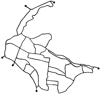
Figure 3: Road network of Rabka. Roads are divided into $374$ approximately equal sections. The black dots mark the exit/entrance roads.

  if $s=0$ then

     if $L_{n}=0$ then

        $0\xrightarrow{P=p\dfrac{w}{2}}1$

     else

        $0\xrightarrow{P=\dfrac{\sum\limits_{out}s}{k_{out}}\dfrac{w}{2}}1$

     end if

  else

     if $L_{n}=0$ then

        $1\xrightarrow{P=v(1-p)}0$

     else

        $1\xrightarrow{P=v\sum\limits_{out}(1-s)}0$

     end if

  end if

Figure 4: Algorithm of a change of the state of the road for a real network.

In the algorithm presented in Fig.4 summing goes through the states of the roads outgoing from a given one, and $k_{out}$ is a number of outgoing roads.

4 Results

4.1 The square lattice

All presented results are a time average in the steady state over $100$ realizations for the square lattice of the size $N=100\times 100$. To check that the results do not depend on the initial conditions, we use three options for the initial state: states of all roads set to $0$, states of all roads set to $1$, and a state of each road is set randomly to be $0$ or $1$.
The results depend on the values of the model parameters $p$, $w$ and $v$. As a result for the whole system the percentage of roads in the state $0$ ($\#0[\%]$) is calculated. The higher the number of zeros the more passable the system is. The results for two different values of the parameter $p$ are presented in Fig. 5 for $p=0.1$ and for $p=0.7$.

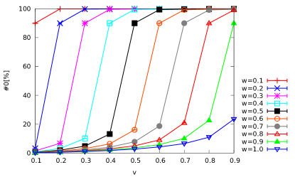
(a) $p=0.1$

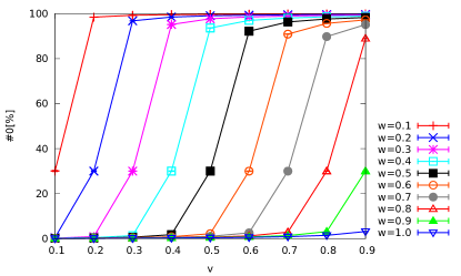
(b) $p=0.7$

Figure 5: Diagram for the square lattice of the size $100\times 100$ (average in the steady state over $100$ realizations).

The increase of the percentage of zeros with the parameter $v$, visible in Fig.5, can be interpreted as an indication of a phase transition. To verify its sharpness dependence on the system size, we calculated the curve $\#0$ vs $v$ for a selected case: $p=0.7$, $w$=0.5 and various system sizes $N^{2}$. The results are shown in Fig.6. Indeed, the sharpness increases with $N$, and the curve for $N=200$ is close to the step function.

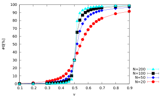
Figure 6: Percentage of zeros in a function of $v$ for square lattices of different sizes $N\times N$ for $p=0.7$ and $w=0.5$ (average in the steady state over $100$ realisations).

We also check how removal of some number of roads changes the obtained results, to check if the symmetry of the square lattice is necessary. In Fig.7 the results obtained when $10\%$ randomly chosen road sections is removed. The removal is done separately for each realization. If, in a consequence of the removal, some part of lattice is isolated, it is removed as well. The results, shown in Fig.7, indicate that the phase transition, found for the square lattice, is observed also in a randomized lattice. The maximal number of zeros in this case is less than 90 percent, because the plot is normalized to the whole square lattice, including the removed links.

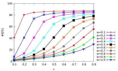
(a) $p=0.1$

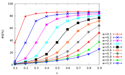
(b) $p=0.7$

Figure 7: Diagram for the square lattice of the size $100\times 100$ (average in the steady state over $100$ realisations), with removal of $10\%$ randomly chosen road sections.

4.2 Small city

The result obtained for the simulations of the traffic network in Rabka, formed by $374$ road sections, are presented in Figs.8. The main difference between this network, as constructed from the map in Fig.3, and the square lattice (with removals or not) is that the Rabka network is less connected. There, often the road sections form long chains. Comparing Figs.5 and 7 we see that the consequence of this difference is that jammed state is less likely. The origin of this result is that jams are created behind the jammed road sections; the more in-neighbors of these sections, the more jams appear. Besides of that, the obtained plot are similar to those for the square lattice.

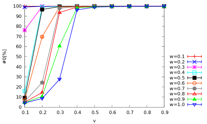
(a) $p=0.1$

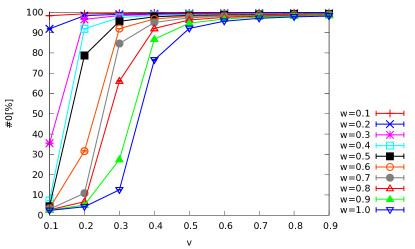
(b) $p=0.7$

Figure 8: Diagram for the real network of the size $N=374$.

4.3 A simplified map

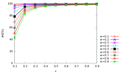
(a) $p=0.1$

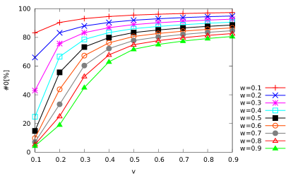
(b) $p=0.7$

Figure 9: Diagram for the real reduced network of the size $N=18$.

Exact calculations of $P(0)$ can be performed merely for systems much smaller than hundreds of road sections. For the sake of comparison of the methods, we simplified the map of Rabka leaving only nine two-way roads. This leads to the system of $2^{18}$ states. The results of the simulations for this system are shown in 9. As the system is much simplified, the results for the full (Fig.8) and reduced (Fig.9) traffic networks differ substantially for $p=0.1$. Surprisingly, those for $p=0.7$ are quite similar. The same simplified network is solved exactly by the solution of $2^{18}=262144$ Master equations [21] for the stationary state for different sets of the model parameters of the related Kripke structure. In this exact method, the parameters $p,v,w$ enter to the weights of links between states, or - equivalently - to the rates of the processes which drive the system from one state to another. For each case we can then calculate, in accordance with Eq.1, the mean stationary probability that the road sections are passable. Obtained results are presented in Figs.10. The same figure shows the solution for the classes of states, as described in [17, 18]. In this case, the class identification procedure allows for the reduction of the system size about twice, to $102400$ classes.

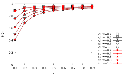
(a) $p=0.1$

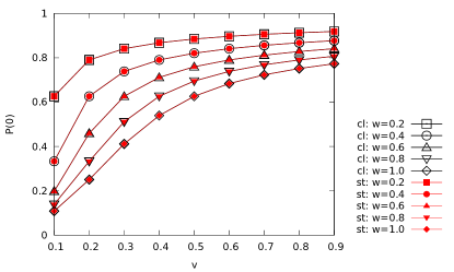
(b) $p=0.7$

Figure 10: Diagram for the real reduced network of the size $N=18$, obtained from the analysis of the state space. Here cl refers to the network of classes, and st to the network of states.

5 Discussion

The goal of this paper is to describe large traffic networks with a cellular automaton, where states of road sections are reduced to two: passable and jammed. The coarse-grained character of the new automaton is close in spirit to the percolation effect. The results of our simulations allow to identify a phase transition between two macroscopic phases, again passable and jammed. Additionally, the calculations are repeated for a much smaller traffic network, constructed by a strong simplification of a map of a small Polish city. These calculations are performed to compare the results with the exact solution of the stationary state, obtained by two equivalent methods. This comparison suggests, that the accordance of simulation with the exact solution is better for more jammed systems, i.e. more close to the phase transition.

The drawback of our automaton is that all information about specific local conditions of traffic jams cannot be reproduced. The model captures merely the jam spreading. The parameters $w$ and $p$ depend on the external state, and serve as an input for the calculations. The parameter $v$ should be calibrated separately for each traffic system. After this calibration, the main result of the model - the probability of the jammed phase - should be reproducible and useful to control the traffic phases. The advantage of the model is its simplicity, which allows to to simulate larger traffic systems in real time.

Acknowledgement: The research is partially supported within the FP7 project SOCIONICAL, No. 231288 and by the Polish Ministry of Science and Higher Education and its grants for Scientific Research and by PL-Grid Infrastructure.

References

- [1] D. Chowdhury, L. Santen and A. Schadschneider, Statistical physics of vehicular traffic and some related systems, Phys. Reports 329 (2000) 199.
- [2] D. Helbing, Traffic and related self-driven many-particle systems, Rev. Mod. Phys. 73 (2001) 1067.
- [3] T. Nagatani, The physics of traffic jams, Rep. Prog. Phys. 65 (2002) 1331.
- [4] S. Maerivoet and B. De Moor, Cellular automata models of road traffic, Phys. Reports 419 (2005) 1.
- [5] Zhu Zhen-Tao, Zhou Jing, Li Ping and Chen Xing-Guang, An evolutionary model of urban bus transport network based on B-space, Chinese Physics B 17 (2008) 2874.
- [6] Gao Zi-You and Li Ke-Ping, Evolution of traffic flow with scale-free topology, Chinese Phys. Lett. 22 (2005) 2711.
- [7] Jian-Feng Zheng and Zi-You Gao, A weighted network evolution with traffic flow, Physica A 387 (2008) 6177.
- [8] S. Kripke, Semantical considerations on modal logic, Acta Philosophica Fennica, 16 (1963) 83.
- [9] R. V. Donner, Yong Zou, J. F. Donges, N. Marvan and J. Kurths, Recurrence networks - a novel paradigm for nonlinear time series analysis, New J. Phys. 12 (2010) 033025.
- [10] T. van Woensel and N. Vandaele, Modelling traffic flows with queueing models: a review, Asia-Pacific Journal of Operational Research 24 (2007) 435.
- [11] C. F. Daganzo, The cell transmission model: a dynamic representation of highway traffic consistent with the hydrodynamic theory, Transportation Research B 28 (1994) 269.
- [12] C. F. Daganzo, The cell transmission model. Part II: Network traffic, Transportation Research B 29 (1995) 79.
- [13] B. Kerner and H. Rehborn, Experimental properties of complexity in traffic flow, Phys. Rev. E 53 (1996) R4275.
- [14] D. Helbing, Empirical traffic data and their implications for traffic modeling, Phys. Rev. E 55 (1997) R25.
- [15] B. S. Kerner, Experimental features of self-organization in traffic flow, Phys. Rev. Lett. 81 (1998) 3797.
- [16] L. Neubert, L. Santen, A. Schadschneider and M. Schreckenberg, Single-vehicle data of highway traffic: a statistical analysis, Phys. Rev. E 60 (1999) 6480.
- [17] M. J. Krawczyk, Topology of space of periodic ground states in antiferromagnetic Ising and Potts models in selected spatial structures, Phys. Lett. A 374 (2010) 2510.
- [18] M. J. Krawczyk, Symmetry induced compression of discrete phase space, Physica A 390 (2011) 2181.
- [19] M. Treiber, A. Hennecke and D. Helbing, Congested traffic states in empirical observations and microscopic simulations, Phys. Rev. E 62 (2000) 1805.
- [20] D. Helbing and K. Nagel, The physics of traffic and regional development, Contemporary Physics 45 (2004) 405.
- [21] N. G. van Kampen, Stochastic Processes in Physics and Chemistry, 3-rd edition, Elsevier, Amsterdam 2007.
- [22] O. Biham, A. A. Middleton and D. Levine, Self-organization and a dynamical transition in traffic-flow models, Phys. Rev. A 46 (1992) R6124.