Incoherent light as a control resource:
a route to complete controllability of quantum systems

Abstract

We discuss the use of incoherent light as a resource to control the atomic dynamics and review the proposed in Phys. Rev. A 84, 042106 (2011) method for a controlled transfer between any pure and mixed states of quantum systems using a combination of incoherent and coherent light. Formally, the method provides a constructive proof for an approximate open-loop Markovian state-transfer controllability of quantum system in the space of all density matrices—the strongest possible degree of quantum state control.

1 Introduction

Optical control of quantum dynamics plays a key role in quantum information and quantum technology [1]. Commonly manipulation by quantum systems is realized using coherent shaped laser pulses [2, 3, 4, 5, 6]. In recent years various methods exploiting incoherent environments as control resources for quantum information and quantum technology were suggested [7, 8, 9, 10, 11, 12]. In this work we discuss the potential for using incoherent light as a control resource for manipulating quantum systems as proposed in [7, 8] and review the method for a controlled deterministic open-loop transfer between arbitrary pure and mixed states using a special combination of incoherent and coherent photons [13]—a result having a fundamental interest as proving the possibility of achieving the maximal degree of quantum state control and practical interest for possible applications in quantum computing with mixed states [14, 15], where engineering of arbitrary density matrices is a necessary component.

Section 2 of this work discusses the notions of coherent and incoherent controls; the former is commonly realized by shaped laser pulses while the latter by tailored state of the environment (for example, by spectral density of incoherent light). Section 3 outlines the proposed physical scheme for steering an arbitrary initial atomic pure or mixed state into vicinity of any final pure or mixed state. This scheme includes two stages, incoherent (described in Section 3.1) and coherent (described in Section 3.2) and proposes a laboratory realization of controllability of open quantum systems in the space of all density matrices. Both stages are equally important for the efficient work of this scheme. Section 3.3 considers as an example the application of this scheme for preparation of a special mixture of $4^{1}S$ and $4^{1}P$ states of Ca atoms. Section 4 explains why our scheme practically proves complete controllability of Markovian quantum systems in the space of all density matrices.

2 Coherent and incoherent controls

Consider an open, that is, interacting with an environment, $n$-level quantum system evolving under the action of a shaped laser pulse $u(t)$. Quantum mechanical state of the system at time $t$ is described by a density matrix $\rho_{t}$ which is a positive matrix with unit trace. Let ${\cal D}_{n}=\{\rho\in\mathbb{C}^{n\times n}\,|\,\rho\geq 0,{\rm Tr}\rho=1\}$, where ${\rm Tr}$ denotes trace, be the set of all density matrices for an $n$-level quantum system.

On a sufficiently short time scale the decoherence effects can be neglected and the laser pulse induces the unitary system dynamics governed by the equation

$$\dot{\rho}_{t}=-i\left[H_{0}+Vu(t),\rho_{t}\right]$$ (1)

Here $H_{0}=\sum\limits_{i=1}^{n}\varepsilon_{i}|i\rangle\langle i|$ is the free Hamiltonian of the system ($\varepsilon_{1}\leq\varepsilon_{2}\leq\dots\leq\varepsilon_{n}$) and $V=-\mu$, where $\mu$ is the dipole moment.

On the long time scale the influence of the environment becomes essential. Commonly, the environment is considered as fixed and having deleterious effects on the system, and moreover its action on the system is assumed to be out of our control. However, this assumption is too restrictive since we can manipulate the state of the environment by adjusting its temperature, pressure or, more generally, its distribution function $n_{\omega}$. Here we consider a simple case when the environment is characterized by the distribution of its particles in energy $\omega$. If the environment is Markovian, then the reduced dynamics of the system density matrix will be governed by the master equation

$$\dot{\rho}_{t}=-i\left[H_{0}+H_{n_{\omega}},\rho_{t}\right]+{\cal L}_{n_{\omega}}(\rho_{t})$$ (2)

where the Lindblad superoperator ${\cal L}_{n_{\omega}}$ is determined by the type of the environment, its state ${n_{\omega}}$, and the microscopic details of its interaction with the system. One particularly convenient environment is spectrally filtered incoherent light [7]. The Lindblad superoperator induced by incoherent light with spectral density ${n_{\omega}}$ (the distribution of photons in frequency $\omega$) has the form

$${\cal L}_{n_{\omega}}(\rho)=\sum\limits_{i<j}A_{ij}\left[(n_{\omega_{ij}}+1)L_{Q_{ij}}(\rho)+n_{\omega_{ij}}L_{Q_{ji}}(\rho)\right]$$

where $A_{ij}\geq 0$ are the Einstein coefficients for spontaneous emission, $\omega_{ij}=\varepsilon_{i}-\varepsilon_{j}$ are the system transition frequencies, $Q_{ij}=|i\rangle\langle j|$ is the transition operator for the $|j\rangle\to|i\rangle$ transition, and $L_{Q}(\rho)=2Q\rho Q^{\dagger}-Q^{\dagger}Q\rho-\rho Q^{\dagger}Q$. The intensities $u(t)$ and $n_{\omega}$ of the coherent and incoherent light are the coherent and incoherent controls, respectively.

3 State transfer between arbitrary pure and mixed quantum states

Here we discuss the scheme were incoherent light with some spectral density $n_{\omega}$ is used as a control resource together with a suitable coherent laser field $u(t)$ to approximately implement state transfer between arbitrary pure and mixed states of finite-level quantum systems [13]. The scheme is described below for implementing state transfer to non-degenerate density matrices, i.e., density matrices with all distinct eigenvalues. Such density matrices are dense in the set ${\cal D}_{n}$ of all density matrices and therefore any pure or mixed quantum state can be approximated with arbitrary precision by non-degenerate states. Thus state transfer to such states is sufficient for any practical purpose.

Let $\rho_{\rm f}=\sum p_{i}|\phi_{i}\rangle\langle\phi_{i}|$ be any desired non-degenerate (i.e., $p_{i}\neq p_{j}$ for $i\neq j$) density matrix. Here $p_{i}$ are its eigenvalues and $|\phi_{i}\rangle$ the corresponding eigenvectors. We assume without loss of the generality that $p_{1}>p_{2}>\dots>p_{n}$. The scheme for steering arbitrary initial density matrix $\rho_{\rm i}$ into $\rho_{\rm f}$ involves the two stages:

• First stage (incoherent): steering $\rho_{\rm i}$ to the state $\tilde{\rho}_{\rm f}=\sum p_{i}|i\rangle\langle i|$ using spectrally filtered incoherent light. The state $\tilde{\rho}_{\rm f}$ has the same eigenvalues as the target state $\rho_{\rm f}$ but is diagonal in the basis of eigenvectors of $H_{0}$. Note also that the populations of the energy levels are arranged in the decreasing order since $p_{1}>p_{2}>\dots>p_{n}$.

• Second stage (coherent): unitary rotation of the basis $\{|i\rangle\}$ to match the basis $\{|\phi_{i}\rangle\}$ of $\rho_{\rm f}$ using coherent laser field. This stage is standard in coherent control.

3.1 Incoherent stage

For this stage we assume that all system transition frequencies $\omega_{ij}$ are different and all $A_{ij}\neq 0$. These assumptions represent the case of general position in the sense that randomly chosen $H_{0}$ and $A_{ij}$ with probability one will satisfy these assumptions. (However, as often might happen with the case of general position there may be important physical examples which do not fit these assumptions.) Under these assumptions any pair of the system states can be independently addressed by incoherent light. During this stage we switch off coherent control so that $u(t)=0$ and apply incoherent control with the optimal spectral density $n_{\omega}$ which has the constant value $n_{\omega_{ij}}=p_{j}/(p_{i}-p_{j})$ in each frequency range of significant absorption and emission for every system transition frequency $\omega_{ij}$. This incoherent control will exponentially fast drive any initial system density matrix $\rho_{\rm i}$ to $\tilde{\rho}_{\rm f}$:

$$\rho_{\rm i}\to\rho_{t}\to\tilde{\rho}_{\rm f}\qquad(t\to\infty)$$

While the complete steering is generally achieved in infinite time, because of the exponential convergence the time period of several magnitudes of the characteristic relaxation time $\tau_{\rm rel}$ is always practically sufficient to be in a desired close proximity of $\tilde{\rho}_{\rm f}$. We apply the control $n_{\omega}$ during such a period and then proceed to the coherent stage.

3.2 Coherent stage

This stage is a standard unitary rotation. The system is assumed to be unitary controllable on a short w.r.t. $\tau_{\rm rel}$ time scale (i.e., such that any unitary evolution operator $U$ can be produced by some fast control). The conditions for unitary controllability of quantum systems are well-known [16]. Incoherent control is switched off during this stage (i.e., $n_{\omega}\equiv 0$) and a fast coherent control with optimal laser pulse $u(t)$ is applied to produce a unitary operator $U_{*}$ transforming the basis $\{|i\rangle\}$ into $|\phi_{i}\rangle$, i.e. such that $U_{*}|i\rangle=|\phi_{i}\rangle$. This stage is realized on a short w.r.t. $\tau_{\rm rel}$ time scale when the decoherence effects are negligible. The system state will evolve as:

$$\tilde{\rho}_{\rm f}\to U^{\vphantom{\dagger}}_{*}\tilde{\rho}_{\rm f}U^{\dagger}_{*}=\rho_{\rm f}$$

As the result of this evolution the system state is steered in the desired state $\rho_{\rm f}$. This dynamics is approximate since even for $n_{\omega}=0$ the spontaneous emission will induce some non-unitary effects. However, these effects are negligible on a sufficiently short w.r.t. $\tau_{\rm rel}$ time scale where unitary dynamics serves as a good approximation. This transformation finishes steering $\rho_{\rm i}$ to $\rho_{\rm f}$.

3.3 Example: Calcium atom

As a testing example we numerically studied in [13] application of control by incoherent light for engineering a mixed state of two calcium levels $|0\rangle=\rm 4^{1}S$ and $|1\rangle=\rm 4^{1}P$. The corresponding transition frequency is $\omega_{21}=4.5\times 10^{15}$ rad/s, the radiative lifetime $t_{21}=4.5$ ns, the Einstein coefficient $A_{21}=1/t_{21}\approx 2.2\times 10^{8}$ s^-1, and the dipole moment $\mu_{12}=2.4\times 10^{-29}$ C$\cdot$m. The method works for any initial and target states; we choose $\rho_{\rm i}=|0\rangle\langle 0|$ and $\rho_{\rm f}=\frac{1}{4}|0\rangle\langle 0|+\frac{3}{4}|1\rangle\langle 1|$ with greater population in the upper state.

During the first (incoherent) stage we prepare the mixture $\tilde{\rho}_{\rm f}=\frac{3}{4}|0\rangle\langle 0|+\frac{1}{4}|1\rangle\langle 1|$ by applying incoherent light with spectral density $n_{\omega_{21}}=1/2$ during the time interval $T=50$ ns. The second (coherent) stage is realized by applying a resonant $\pi$-pulse $E(t)=E\cos(\omega_{12}t)$ with amplitude $E=10^{7}$ V/m acting during the time interval $T_{\rm f}-T=1310$ fs (other coherent control methods producing the same unitary transformation can be used as well); this field has the Rabi frequency $\Omega_{\rm R}\approx 1/2320$ fs^-1 and acts as a $\pi$-pulse transforming the state $\tilde{\rho}_{\rm f}$ into $\rho_{\rm f}$. The results of the numerical simulation are shown in Fig. 1.

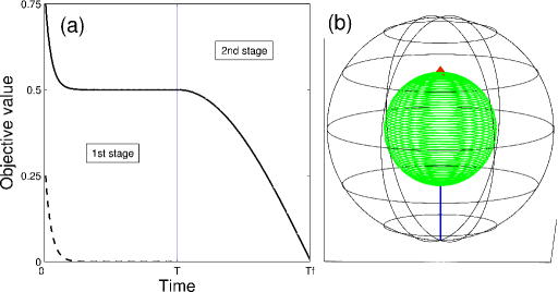
Figure 1: (From Ref. [13]. Copyright (2011) by the American Physical Society.) The results of the numerical simulations for engineering a target mixed state $\rho_{\rm f}=\frac{1}{4}|0\rangle\langle 0|+\frac{3}{4}|1\rangle\langle 1|$ of two Ca energy levels. (a) The behavior of $\|\rho_{t}-\rho_{\rm f}\|$ (solid line) and $\|\rho_{t}-\tilde{\rho}_{\rm f}\|$ (dashed line) during the two control stages. The time scale is not uniform: $T=50$ ns and $T_{\rm f}-T=1310$ fs. (b) The corresponding evolution of the Bloch vector showing that the evolved state approaches the target state (red marker at the top).

4 Complete controllability of quantum systems

A fundamental property of any control system is the degree of its controllability. The state of the system is a collection of the system’s variables which completely describes the system at any given time. Complete state controllability (or simply controllability) describes the ability to steer with the available controls any initial state of the system into any final state. For quantum mechanical systems the state space can be either the set of all pure states, or any complete set of density matrices with the same eigenvalues (i.e., any complete set of kinematically equivalent density matrices), or the set of all density matrices ${\cal D}_{n}$. The latter set is the biggest and contains as subsets the two former sets. Therefore state controllability in ${\cal D}_{n}$ is the strongest amongst all notions of quantum state control; controllability of a given quantum system in ${\cal D}_{n}$ implies its controllability in the space of pure states and in the space of kinematically equivalent density matrices.

The method of [13] which is described in section 3 of this paper allows to steer an arbitrary initial state into a vicinity of an arbitrary final state. While the definition of controllability requires exact steering, for practical purposes it is always sufficient to steer the system into some vicinity of the final state. Thus our method practically proves the strongest degree of state controllability of quantum systems—controllability in the space of all density matrices ${\cal D}_{n}$. A powerful method for proving controllability of bilinear systems is the Lie algebraic method. The proof in [13] is different: we prove controllability by explicitly constructing optimal controls which steer any initial state into any given final state. The success in finding these controls is due to a special structure of the Markovian master equation describing interaction of a quantum system with incoherent light. An important feature of our method is that we use a physical environment comprised of incoherent photons and its spectral density is accessible to manipulate. Another feature is that the proposed method does not use simultaneous control by coherent and incoherent fields. This property is important because deriving a correct master equation with simultaneous time dependent Hamiltonian and a dissipative term is a non-trivial problem. Simple addition of ${\cal L}_{n_{\omega}}$ to the r.h.s. of eq. (1) may lead to an incorrect equation because time dependent Hamiltonian can also modify the non-Hamiltonian part ${\cal L}_{n_{\omega}}$. In our method both controls are separated in time that allows to avoid this problem and assures that we use a correct description of the dynamics. Recently several works have appeared which also analyze and prove controllability of quantum systems controlled by a coherent control with a Markovian environment. The preprint [17] uses a Lie algebraic technique and the preprint [18] uses coherent control and a switchable noise to transfer between arbitrary states of $n$-level quantum systems.

References

- [1] A. V. Sergienko, ed. Quantum Communications and Cryptography (CRC Press, 2006).
- [2] D. J. Tannor and S. A. Rice, “Control of selectivity of chemical reaction via control of wave packet evolution”, J. Chem. Phys. 83, 5013–5018 (1985).
- [3] P. W. Brumer and M. Shapiro, Principles of the Quantum Control of Molecular Processes (Wiley, 2003).
- [4] V. S. Letokhov, Laser Control of Atoms and Molecules (Oxford University Press, USA, 2007).
- [5] D. V. Zhdanov and V. N. Zadkov, “Laser-assisted control of molecular orientation at high temperatures”, Phys. Rev. A 77, 011401(R) (2008).
- [6] U. Steinitz, Y. Prior, and I. Sh. Averbukh, “Laser-induced gas vortices”, Phys. Rev. Lett. 109, 033001 (2012).
- [7] A. Pechen and H. Rabitz, “Teaching the environment to control quantum systems”, Phys. Rev. A 73, 062102 (2006).
- [8] A. Pechen and H. Rabitz, “Incoherent control of open quantum systems”, Reports of the Samara State University: Natural Science Series 8(1), 641–658 (2008).
- [9] F. Verstraete, M. M. Wolf, J. I. Cirac, “Quantum computation and quantum-state engineering driven by dissipation”, Nature Physics 5, 633–636 (2009).
- [10] H. Weimer, M. Müller, I. Lesanovsky, P. Zoller, and H. P. Büchler, “A Rydberg quantum simulator”, Nature Physics 6, 382–388 (2010).
- [11] J. T. Barreiro, P. Schindler, O. G hne, T. Monz, M. Chwalla, C. F. Roos, M. Hennrich, R. Blatt, “Experimental multiparticle entanglement dynamics induced by decoherence”, Nature Physics 6, 943–946 (2010).
- [12] D. Rossini, T. Calarco, V. Giovannetti, S. Montangero, R. Fazio, “Decoherence induced by interacting quantum spin baths”, Phys. Rev. A 75, 032333 (2007).
- [13] A. Pechen, “Engineering arbitrary pure and mixed quantum states”, Phys. Rev. A 84, 042106 (2011).
- [14] D. Aharonov, A. Kitaev, N. Nisan, “Quantum circuits with mixed states”, in Proceedings of 13th Annual ACM Symposium on Theory of Computation (STOC, 1997), pp 20–30; arXiv:quant-ph/9806029 ).
- [15] V. E. Tarasov, “Quantum computer with mixed states and four-valued logic”, J. Phys. A 35, 5207–5235 (2002).
- [16] V. Ramakrishna, M. V. Salapaka, M. Dahleh, H. Rabitz, A. Pierce, “Controllability of molecular systems”, Phys. Rev. A 51, 960 (1995).
- [17] A. Grigoriu, H. Rabitz, and G. Turinici, “Controllability analysis of quantum systems immersed within an engineered environment”, Preprint hal-00696546, v. 3 (2012).
- [18] V. Bergholm and T. Schulte-Herbrüggen, “How to transfer between arbitrary n-qubit quantum states by coherent control and simplest switchable noise on a single qubit”, arXiv:1206.4945 (2012).