Gradient-based stochastic optimization methods in
Bayesian experimental design

Abstract

Optimal experimental design (OED) seeks experiments expected to yield the most useful data for some purpose. In practical circumstances where experiments are time-consuming or resource-intensive, OED can yield enormous savings. We pursue OED for nonlinear systems from a Bayesian perspective, with the goal of choosing experiments that are optimal for parameter inference. Our objective in this context is the expected information gain in model parameters, which in general can only be estimated using Monte Carlo methods. Maximizing this objective thus becomes a stochastic optimization problem.

This paper develops gradient-based stochastic optimization methods for the design of experiments on a continuous parameter space. Given a Monte Carlo estimator of expected information gain, we use infinitesimal perturbation analysis to derive gradients of this estimator. We are then able to formulate two gradient-based stochastic optimization approaches: (i) Robbins-Monro stochastic approximation, and (ii) sample average approximation combined with a deterministic quasi-Newton method. A polynomial chaos approximation of the forward model accelerates objective and gradient evaluations in both cases. We discuss the implementation of these optimization methods, then conduct an empirical comparison of their performance. To demonstrate design in a nonlinear setting with partial differential equation forward models, we use the problem of sensor placement for source inversion. Numerical results yield useful guidelines on the choice of algorithm and sample sizes, assess the impact of estimator bias, and quantify tradeoffs of computational cost versus solution quality and robustness.

1 Introduction

Experimental data play a crucial role in the development of models—and the advancement of scientific understanding—across a host of disciplines. Some experiments are more useful than others, however, and a careful choice of experiments can translate to enormous savings of time and financial resources. Traditional experimental design methods, such as factorial and composite designs, are largely used as heuristics for exploring the relationship between input factors and response variables. Optimal experimental design, on the other hand, uses a model to guide the choice of experiments for a particular purpose, such as parameter inference, prediction, or model discrimination. Optimal design has seen extensive development for linear models endowed with Gaussian distributions [1]. Extensions to nonlinear models are often based on linearization and Gaussian approximations [2, 3, 4], as analytical results are otherwise impractical or impossible to obtain. With advances in computational power, however, optimal experimental design for nonlinear systems can now be tackled directly using numerical simulation [5, 6, 7, 8, 9, 10, 11].

This paper pursues nonlinear experimental design from a Bayesian perspective (e.g., [12]). The Bayesian statistical approach [13, 14] provides a rigorous foundation for inference from noisy, indirect, and incomplete data and a natural mechanism for incorporating physical constraints and heterogeneous sources of information. We focus on experiments described by a continuous design space, with the goal of choosing experiments that are optimal for Bayesian parameter inference. A useful objective function for this purpose is the expected information gain in model parameters [15, 16]—or equivalently, the mutual information between parameters and observables, conditioned on the design variables. This objective can be derived in a decision theoretic framework, using the Kullback-Leibler divergence from posterior to prior as a utility function [4]. From the numerical perspective, however, it is a complicated quantity. In general, it must be approximated using a Monte Carlo method [6, 17]. Consequently, only noisy estimates of the objective function are available and the optimal design problem becomes a stochastic optimization problem.

There are many approaches for solving continuous optimization problems with stochastic objectives. While some do not require the direct evaluation of gradients (e.g., Nelder-Mead [18], Kiefer-Wolfowitz [19], and simultaneous perturbation stochastic approximation [20]), other algorithms can use gradient evaluations to great advantage. Broadly, these algorithms involve either stochastic approximation (SA) [21] or sample average approximation (SAA) [22], where the latter approach must also invoke a gradient-based deterministic optimization algorithm. Hybrids of the two approaches are possible as well. In either case, for model-based experimental design, one must employ gradients of the information gain objective described above. This objective function itself involves nested integrations over possible model outputs and over the input parameter space, where the model output may be a functional of the solution of a partial differential equation. In many practical cases, the model may be essentially a black box; while in other cases, even if gradients can be evaluated with adjoint methods, using the full model to evaluate the expected information gain or its gradient is computationally prohibitive. Previous work [11] has addressed these difficulties by constructing polynomial surrogates for the the model output, i.e., polynomial chaos expansions [23, 24, 25, 26, 27, 28, 29] that capture dependence on both uncertain parameters and design variables.

The main contributions of this paper are as follows. First, we show how to use infinitesimal perturbation analysis to derive gradients of a Monte Carlo estimator of the expected information gain. When the estimator incorporates a polynomial surrogate, we show how this surrogate can be readily extended to provide analytical gradient estimates. We then conduct a systematic empirical comparison of two gradient-based stochastic optimization approaches for nonlinear experimental design: (1) Robbins-Monro (RM) stochastic approximation, and (2) sample average approximation combined with a deterministic quasi-Newton method. The comparison is performed in the context of a physics-based sensor placement application, where the forward model is given by a partial differential equation. From the numerical results, we are able to assess the impact of estimator bias, extract useful guidelines on the choice of algorithm and sample sizes, and quantify tradeoffs of computational cost versus solution quality and robustness.

The RM algorithm [30] is the original and perhaps most widely used stochastic approximation method, and has become a prototype for many subsequent algorithms. It involves an iterative update that resembles steepest descent, except that it uses stochastic gradient information. Sample average approximation (SAA) (also known as the retrospective method [31] or the sample-path method [32]) is a more recent approach, with theoretical analysis initially appearing in the 1990s [22, 32, 33]. Convergence rates and stochastic bounds, although useful, do not necessarily reflect empirical performance under finite computational resources and with imperfect numerical optimization schemes. To the best of our knowledge, extensive numerical testing of SAA has focused on stochastic programming problems with special structure (e.g., linear programs with discrete design variables) [34, 35, 36, 37, 38]. While numerical improvements to SAA have seen continual development (e.g., estimators of optimality gap [39, 40] and sample size adaptation [41, 42]), the practical behavior of SAA in more general optimization settings is largely unexplored. The numerical assessment of SAA conducted here, in a nonlinear and continuous variable design setting, is thus expected to be of practical interest.

SAA is frequently compared to stochastic approximation methods such as RM. For example, [43] suggests that SAA is more robust than SA because of sensitivity to step size choice in the latter. On the other hand, variants of SA have been developed that, for certain classes of problems (e.g., [44]), reach solution quality comparable to that of SAA in substantially less time. The comparison of SA and SAA presented here focuses on their performance in the Bayesian experimental design problem. We do not aim to identify one approach as superior to the other; instead, we will simply illustrate the differences between the two algorithms in this context and provide some selection guidelines based on their properties.

This paper is organized as follows. Section 2 introduces optimal Bayesian experimental design (§2.1) and extracts the underlying stochastic optimization problem (§2.2), then presents the RM (§2.2.1) and SAA-BFGS (§2.2.2) algorithms. The challenge of evaluating gradient information appropriate to each of these algorithms is described in Section 2.3. Section 3 and Section 4 describe how to obtain gradients (or gradient estimators) for the experimental design objective using polynomial chaos expansions and infinitesimal perturbation analysis. Section 5 then analyzes the numerical performance of RM and SAA-BFGS on an optimal sensor placement problem involving contaminant diffusion. Conclusions on the algorithms and the relative strengths of SA and SAA for optimal experimental design are provided in Section 6.

2 Optimal Bayesian Experimental Design

2.1 Background

We are interested in choosing the “best” experiments from a continuously parameterized design space, for the purpose of inferring model parameters from noisy and indirect observations. In other words, we seek experiments that are optimal for parameter inference (in a sense to be precisely defined below), with inference performed in a Bayesian setting. In the problems considered here, the mean observations are nonlinear functions of the model parameters, and the observations and model parameters are continuous random variables.

Bayes’ rule describes the parameter update process:

$$f_{\bm{\Theta}|\mathbf{Y},\mathbf{d}}(\bm{\theta}|\mathbf{y},\mathbf{d})=\frac{f_{\mathbf{Y}|\bm{\Theta},\mathbf{d}}(\mathbf{y}|\bm{\theta},\mathbf{d})f_{\bm{\Theta}|\mathbf{d}}(\bm{\theta}|\mathbf{d})}{f_{\mathbf{Y}|\mathbf{d}}(\mathbf{y}|\mathbf{d})}.$$ (1)

Here $\bm{\Theta}$ represents the uncertain parameters of interest, $\mathbf{Y}$ the observations, and $\mathbf{d}$ the design variables. Like the observations and parameters, the design parameters are continuous. Also $f_{\bm{\Theta}|\mathbf{d}}$ is the prior density, $f_{\mathbf{Y}|\bm{\Theta},\mathbf{d}}$ is the likelihood function, $f_{\bm{\Theta}|\mathbf{Y},\mathbf{d}}$ is the posterior density, and $f_{\mathbf{Y}|\mathbf{d}}$ is the evidence. It is reasonable to assume that prior knowledge on $\bm{\Theta}$ does not vary with the design choice, leading to the simplification $f_{\bm{\Theta}|\mathbf{d}}(\bm{\theta}|\mathbf{d})=f_{\bm{\Theta}}(\bm{\theta})$.

Taking the decision theoretic approach proposed by Lindley [15, 16], we use the Kullback-Leibler (KL) divergence [45, 46] from the posterior to the prior as a utility function, and take its expectation under the prior predictive distribution of the data to obtain an expected utility $U(\mathbf{d})$:

$$U(\mathbf{d}) = \int_{\mathcal{Y}}\int_{\mathcal{H}}f_{\bm{\Theta}|\mathbf{Y},\mathbf{d}}(\bm{\theta}|\mathbf{y},\mathbf{d})\ln\left[\frac{f_{\bm{\Theta}|\mathbf{Y},\mathbf{d}}(\bm{\theta}|\mathbf{y},\mathbf{d})}{f_{\bm{\Theta}}(\bm{\theta})}\right]\,d\bm{\theta}\,f_{\mathbf{Y}|\mathbf{d}}(\mathbf{y}|\mathbf{d})\,d\mathbf{y}$$

$$= \mathbb{E}_{\mathbf{Y}|\mathbf{d}}\left[D_{\mathrm{KL}}\left(f_{\bm{\Theta}|\mathbf{Y},\mathbf{d}}(\cdot|\mathbf{Y},\mathbf{d})||f_{\bm{\Theta}}(\cdot)\right)\right].$$

Here $\mathcal{H}$ is the support of $f_{\bm{\Theta}}(\bm{\theta})$ and $\mathcal{Y}$ is the support of $f_{\mathbf{Y}|\mathbf{d}}(\mathbf{y}|\mathbf{d})$. Because the observation $\mathbf{Y}$ cannot be known before the experiment is performed, taking the expectation over the prior predictive $f_{\mathbf{Y}|\mathbf{d}}$ lets the resulting utility function reflect the information gain on average, over all anticipated outcomes of the experiment. The KL divergence may be understood as information gain: larger KL divergence from posterior to prior implies that the data $\mathbf{Y}$ decrease entropy in $\bm{\Theta}$ by a larger amount, and hence are more informative for parameter inference. The expected utility $U(\mathbf{d})$ is thus the expected information gain due to an experiment performed at conditions $\mathbf{d}$, which is equivalent to the mutual information between the parameters $\bm{\theta}$ and the observables $\mathbf{y}$ conditioned on $\mathbf{d}$. A more detailed derivation and discussion can be found in [11].

Typically, the expected utility in (2.1) has no closed form (even if the predictive mean of the data is, for example, a polynomial function of $\bm{\theta}$). Instead, it must be approximated numerically. By applying Bayes’ rule to the quantities inside and outside the logarithm in (2.1), and then introducing Monte Carlo approximations for the resulting integrals, we obtain the nested Monte Carlo estimator proposed by Ryan [6]:

$$U(\mathbf{d})\approx\hat{U}_{N,M}(\mathbf{d},\bm{\theta}_{s},\mathbf{y}_{s})\equiv\frac{1}{N}\sum_{i=1}^{N}\left\{\ln\left[f_{\mathbf{Y}|\bm{\Theta},\mathbf{d}}(\mathbf{y}^{(i)}|\bm{\theta}^{(i)},\mathbf{d})\right]-\ln\left[\frac{1}{M}\sum_{j=1}^{M}f_{\mathbf{Y}|\bm{\Theta},\mathbf{d}}(\mathbf{y}^{(i)}|\tilde{\bm{\theta}}^{(i,j)},\mathbf{d})\right]\right\},$$ (3)

where $\bm{\theta}_{s}\equiv\left\{\bm{\theta}^{(i)}\right\}\cup\left\{\tilde{\bm{\theta}}^{(i,j)}\right\}$, $i=1\ldots N$, $j=1\ldots M$, are i.i.d. samples from the prior $f_{\bm{\Theta}}$; and $\mathbf{y}_{s}\equiv\left\{\mathbf{y}^{(i)}\right\}$, $i=1\ldots N$, are independent samples from the likelihoods $f_{\mathbf{Y}|\bm{\Theta},\mathbf{d}}(\cdot|\bm{\theta}^{(i)},\mathbf{d})$. The variance of this estimator is approximately ${A(\mathbf{d})}/{N}+{B(\mathbf{d})}/{NM}$ and its bias is (to leading order) ${C(\mathbf{d})}/{M}$ [6], where $A$, $B$, and $C$ are terms that depend only on the distributions at hand. While the estimator $\hat{U}_{N,M}$ is biased for finite $M$, it is asymptotically unbiased.

Finally, the expected utility must be maximized over the design space $\mathcal{D}$ to find the optimal experiment(s):

$$\mathbf{d}^{\ast}=\mathrm{arg}\max_{\mathbf{d}\in\mathcal{D}}\,U(\mathbf{d}).$$ (4)

Since $U$ can only be approximated by Monte Carlo estimators such as $\hat{U}_{N,M}$, optimization methods for stochastic objective functions are needed.

2.2 Stochastic optimization

In this section we describe two gradient-based stochastic optimization approaches: Robbins-Monro stochastic approximation, and sample average approximation with the Broyden-Fletcher-Goldfarb-Shanno method. Both approaches require some flavor of gradient information, but they do not use the exact gradient of $U(\mathbf{d})$. Calculating the latter is generally not possible, given that we only have a Monte Carlo estimator (3) of $U(\mathbf{d})$.

For simplicity, in this section only (§2.2), we will use a more generic notation to describe the stochastic optimization problem at hand. This will allow the essential ideas to be presented before tackling the additional complexities of the expected information gain estimator above. The problem to be solved is of the form

$$x^{\ast}=\mathrm{arg}\min_{x\in\mathcal{X}}\,\left\{h(x)=\mathbb{E}_{W}\left[\hat{h}(x,W)\right]\right\},$$ (5)

where $x$ is the design variable, $W$ is the (generally design-dependent) “noise” random variable, and $\hat{h}(x,w)$ is an unbiased estimator of the unavailable objective function $h(x)$.

2.2.1 Robbins-Monro (RM) stochastic approximation

The iterative update of the Robbins-Monro method is

$$x_{k+1}=x_{k}-a_{k}\hat{g}(x_{k},w^{\prime}),$$ (6)

where $k$ is the iteration index and $\hat{g}(x_{k},w^{\prime})$ is an unbiased estimator of the gradient (with respect to $x$) of $h(x)$ evaluated at $x_{k}$. In other words, $\mathbb{E}_{W^{\prime}}\left[\hat{g}(x,W^{\prime})\right]=\nabla_{x}h(x)$, but $\hat{g}$ is not necessarily equal to $\nabla\hat{h}$. Also, $W^{\prime}$ and $W$ may, but need not, be related. The gain sequence $a_{k}$ should satisfy the following properties:

$$\sum_{k=0}^{\infty}a_{k}=\infty \mathrm{and} \sum_{k=0}^{\infty}a_{k}^{2}<\infty.$$ (7)

One natural choice, used in this study, is the harmonic step size sequence $a_{k}={\beta}/{k}$, where $\beta$ is some appropriate scaling constant. For example, in the diffusion problem of Section 5, $\beta$ is chosen to be 1.0 since the design space is $[0,1]^{2}$. With various technical assumptions on $\hat{g}$ and $g$, it can be shown that RM converges to the exact solution of (5) almost surely [21].

Choosing the sequence $a_{k}$ is often viewed as the Achilles’ heel of RM, as the algorithm’s performance can be very sensitive to step size. We acknowledge this fact and do not downplay the difficulty of choosing an appropriate gain sequence, but we will try to show that there exist logical approaches to selecting $a_{k}$ that yield reasonable performance. More sophisticated strategies, such as search-then-converge learning rate schedules [47], adaptive stochastic step size rules [48], and iterate averaging methods [21, 49], have been developed and successfully demonstrated in applications. For simplicity, however, we will use only the harmonic step size sequence in this paper.

We will also use relatively simple stopping criteria for the RM iterations: the algorithm will be terminated when changes in $x_{k}$ stall (e.g., $\|\,x_{k}-x_{k-1}\,\|$ falls below some designated tolerance for 5 successive iterations) or when a maximum number of iterations has been reached (e.g., 50 iterations in the numerical experiments of Section 5.2.2.)

2.2.2 Sample average approximation (SAA)

Transformation to design-independent noise.

The central idea of sample average approximation is to reduce the stochastic optimization problem to a deterministic problem, by fixing the noise throughout the entire optimization process. In practice, if the noise $W$ is design-dependent, it is first transformed to a design-independent random variable by moving all the design dependence into the function $\hat{h}$. (An example of this transformation is given in Section 4.) The noise variables at different $x$ then share a common distribution, and a common set of realizations is employed at all values of $x$.

Such a transformation is always possible in practice, since the random numbers in any computation are fundamentally generated from uniform random (or really pseudorandom) numbers. Thus one can always transform $W$ back into these uniform random variables, which are of course independent of $x$. For the remainder of this section (§2.2.2) we shall, without loss of generality, assume that $W$ is independent of $x$.

Reduction to a deterministic problem.

SAA approximates the true optimization problem in (5) with

$$\hat{x}_{s}=\mathrm{arg}\min_{x\in\mathcal{X}}\left\{\hat{h}_{N}(x,w_{s})\equiv\frac{1}{N}\sum_{i=1}^{N}\hat{h}(x,w_{i})\right\},$$ (8)

where $\hat{x}_{s}$ and $\hat{h}_{N}(\hat{x}_{s},w_{s})$ are the optimal design and objective values under a particular set of $N$ realizations of the random variable $W$, $w_{s}\equiv\{w_{i}\}_{i=1}^{N}$. The same set of realizations is used for different values of $x$ during the optimization process, thus making the minimization problem in (8) deterministic. (One can view this approach as an application of common random numbers.) A deterministic optimization algorithm can then be chosen to find $\hat{x}_{s}$ as an approximation to $x^{\ast}$.

Estimates of $h(\hat{x}_{s})$ can be improved by using $\hat{h}_{N^{\prime}}(\hat{x}_{s},w_{s^{\prime}})$ instead of $\hat{h}_{N}(\hat{x}_{s},w_{s})$, where $\hat{h}_{N^{\prime}}(\hat{x}_{s},w_{s^{\prime}})$ is computed from a larger set of realizations $w_{s^{\prime}}\equiv\{w_{j}\}_{j=1}^{N^{\prime}}$ with $N^{\prime}>N$, in order to attain a lower variance. Finally, multiple (say $T$) optimization runs are often performed to obtain a sampling distribution for the optimal design values and the optimal objective values, i.e., $\hat{x}_{s}^{t}$ and $\hat{h}_{N}(\hat{x}_{s}^{t},w_{s}^{t})$, for $t=1\ldots T$. The sets $w_{s}^{t}$ are independently chosen for each optimization run, but remain fixed within each run. Under certain assumptions on the objective function and the design space, the optimal design and objective estimates in SAA generally converge to their respective true values in distribution at a rate of $1/\sqrt{N}$ [22, 33].

For the solution of a particular deterministic problem $\hat{x}^{t}_{s}$, stochastic bounds on the true optimal value can be constructed by estimating the optimality gap $h(\hat{x}^{t}_{s})-h(x^{\ast})$ [39, 40]. The first term can simply be approximated using the unbiased estimator $\hat{h}_{N^{\prime}}(\hat{x}_{s}^{t},w_{s^{\prime}}^{t})$ since $\mathbb{E}_{W_{s^{\prime}}}\left[\hat{h}_{N^{\prime}}(\hat{x}_{s}^{t},W_{s^{\prime}})\right]=h(\hat{x}_{s}^{t})$. The second term may be estimated using the average of the approximate optimal objective values across the $T$ replicate optimization runs (based on $w_{s}^{t}$, rather than $w_{s^{\prime}}^{t}$):

$$\bar{h}_{N}=\frac{1}{T}\sum_{t=1}^{T}\hat{h}_{N}(\hat{x}_{s}^{t},w_{s}^{t}).$$ (9)

This is a negatively biased estimator and hence a stochastic lower bound on $h(x^{\ast})$ [39, 40, 50].^, The difference $\hat{h}_{N^{\prime}}(\hat{x}_{s}^{t},w_{s^{\prime}}^{t})-\bar{h}_{N}$ is thus a stochastic upper bound on the true optimality gap $h(\hat{x}^{t}_{s})-h(x^{\ast})$. The variance of this optimality gap estimator can be derived from the Monte Carlo standard error formula [34]. One could then use the optimality gap estimator and its variance to decide whether more runs are required, or which approximate optimal designs are most trustworthy.

Pseudocode for the SAA method is presented in Algorithm 1. At this point, we have reduced the stochastic optimization problem to a series of deterministic optimization problems; a suitable deterministic optimization algorithm is still needed to solve them.

Set optimality gap tolerance $\eta$ and number of replicate optimization runs $T$;

$t=1$;

while optimality gap estimate $>\eta$ and $t\leq T$ do

       Sample the set $w_{s}^{t}=\{w_{i}^{t}\}_{i=1}^{N}$;

       Perform a deterministic optimization run and find $\hat{x}_{s}^{t}$ (see Algorithm 2);

       Sample the larger set $w_{s^{\prime}}^{t}=\{w_{j}^{t}\}_{j=1}^{N^{\prime}}$ where $N^{\prime}>N$;

       Compute $\hat{h}_{N^{\prime}}(\hat{x}_{s}^{t},w_{s^{\prime}}^{t})=\frac{1}{N^{\prime}}\sum_{j=1}^{N^{\prime}}\hat{h}\left(\hat{x}_{s}^{t},w_{j}^{t}\right)$;

       Estimate the optimality gap and its variance;

       $t=t+1$;

      

end Output the sets $\{\hat{x}_{s}^{t}\}_{t=1}^{T}$ and $\{\hat{h}_{N^{\prime}}(\hat{x}_{s}^{t},w_{s^{\prime}}^{t})\}_{t=1}^{T}$ for post-processing;

Algorithm 1 SAA method in pseudocode.

BFGS method.

The Broyden-Fletcher-Goldfarb-Shanno (BFGS) method [51] is a gradient-based method for solving deterministic nonlinear optimization problems, widely used for its robustness, ease of implementation, and efficiency. It is a quasi-Newton method, iteratively updating an approximation to the (inverse) Hessian matrix from objective and gradient evaluations at each stage. Pseudocode for the BFGS method is given in Algorithm 2. In the present implementation, a simple backtracking line search is used to find a stepsize that satisfies the first (Armijo) Wolfe condition only. The algorithm can be terminated according to many commonly used criteria: for example, when the gradient stalls, the line search stepsize falls below a prescribed tolerance, the design variable or function value stalls, or a maximum allowable number of iterations or objective evaluations is reached. BFGS is shown to converge super-linearly to a local minimum if a quadratic Taylor expansion exists near that minimum [51].

The limited memory BFGS (L-BFGS) [51] method can also be used when the design dimension becomes very large (e.g., more than $10^{4}$), such that the dense inverse Hessian cannot be stored explicitly.

Initialize starting point $x_{0}$, inverse Hessian approximation $H_{0}$, gradient termination tolerance $\varepsilon$;

Initialize any other termination conditions and parameters;

$k=0$;

while $\|\,\nabla\hat{h}_{N}(x_{k},w_{s}^{t})\,\|>\varepsilon$ and other termination conditions are not met do

       Compute search direction $p_{k}=-H_{k}\nabla\hat{h}_{N}(x_{k},w_{s}^{t})$;

       Find acceptable stepsize $\alpha_{k}$ via line search;

       Update position $x_{k+1}=x_{k}+\alpha_{k}p_{k}$;

       Define vectors $s_{k}=x_{k+1}-x_{k}$ and $u_{k}=\nabla\hat{h}_{N}(x_{k+1},w_{s}^{t})-\nabla\hat{h}_{N}(x_{k},w_{s}^{t})$ ;

       Update inverse Hessian approximation $H_{k+1}=\left(I-\frac{s_{k}u_{k}^{T}}{s_{k}^{T}u_{k}}\right)H_{k}\left(I-\frac{u_{k}s_{k}^{T}}{u_{k}^{T}s_{k}}\right)+\frac{s_{k}s_{k}^{T}}{s_{k}^{T}u_{k}}$;

       $k=k+1$;

      

end Output $\hat{x}_{s}^{t}=x_{k}$;

Algorithm 2 BFGS algorithm in pseudocode. In this context, $\hat{h}_{N}(x,w_{s}^{t})$ is the deterministic objective function we want to minimize (as a function of $x$).

2.3 Application to optimal design

The main challenge in applying the aforementioned stochastic optimization algorithms to optimal Bayesian experimental design is the lack of readily-available gradient information. For RM, we need an unbiased estimator of the gradient of the expected utility, i.e., $\hat{g}$ in (6). For SAA-BFGS, we need the gradient of the finite-sample Monte Carlo approximation of the expected utility, i.e., $\nabla\hat{h}_{N}(\cdot,w_{s}^{t})$.

We address these needs by introducing two concepts:

1. A simple surrogate model, based on polynomial chaos expansions (see Section 3), replaces the often computationally-intensive forward model. The purpose of the surrogate is twofold. First, it allows the nested Monte Carlo estimator (3) to be evaluated in a computationally tractable manner. Second, its polynomial form allows the gradient of (3), $\nabla\hat{h}_{N}(\cdot,w_{s}^{t})$, to be derived analytically. These gains come at the expense of introducing additional error via the polynomial approximation of the original forward model, however. In other words, given a surrogate for the forward model and the resulting expected information gain, we can derive exact gradients of a Monte Carlo approximation of this expected information gain, and use these gradients in SAA.

2. Infinitesimal perturbation analysis (see Section 4) applied to (2.1), along with the estimator in (3) and the polynomial surrogate model, allows the analytical derivation of an unbiased gradient estimator $\hat{g}$, as required for the RM approach.

3 Polynomial chaos surrogates

3.1 Background

This section introduces the first of two computational tools used to address the challenges described in Section 2.3. Polynomial expansions will be used to mitigate the cost of repeated forward model evaluations. Later (see Section 4) they will also be used to help evaluate appropriate gradient information for stochastic optimization methods.

Mathematical models of the experiment enter the inference and design formulation through the likelihood function $f_{\mathbf{Y}|\bm{\Theta},\mathbf{d}}$. For example, a simple likelihood function might allow for an additive discrepancy $\mathbf{E}$ between experimental observations and model predictions

$$\mathbf{Y}=\mathbf{G}(\bm{\Theta},\mathbf{d})+\mathbf{E}.$$ (10)

Here $\mathbf{G}(\bm{\theta},\mathbf{d})$ is the “forward model” describing the experiment; it is a function that maps both the design variables and the parameters into the data space. The discrepancy $\mathbf{E}$ is often taken to be a Gaussian random variable, but is by no means limited to this; we will use $f_{\mathbf{E}}$ to denote its probability density. Computationally intensive forward models can render Monte Carlo estimation of the expected information gain impractical. In particular, drawing a sample from $f_{\mathbf{Y}|\bm{\Theta},\mathbf{d}}(\mathbf{y}|\bm{\theta},\mathbf{d})$ requires evaluating $\mathbf{G}$ at a particular $(\bm{\theta},\mathbf{d})$. Evaluating the density $f_{\mathbf{Y}|\bm{\Theta},\mathbf{d}}(\mathbf{y}|\bm{\theta},\mathbf{d})=f_{\mathbf{E}}(\mathbf{y}-\mathbf{G}(\bm{\theta},\mathbf{d}))$ again requires evaluating $\mathbf{G}$.

To make these calculations tractable, one would like to replace $\mathbf{G}$ with a cheaper “surrogate” model that is accurate over the entire prior support $\mathcal{H}$ and the entire design space $\mathcal{D}$. Many options exist, ranging from projection-based model reduction [52, 53] to spectral methods based on polynomial chaos (PC) expansions [23, 24, 25, 26, 27, 28, 29, 54]. The latter approaches do not reduce the internal physics of the deterministic model; rather, they exploit regularity in the dependence of model outputs on uncertain input parameters and design variables.

Polynomial chaos has seen extensive use in a range of engineering applications (e.g., [55, 56, 57, 58]) including parameter estimation and inverse problems (e.g., [59, 60, 61]). More recently, it has also been used in open-loop optimal Bayesian experimental design [10, 11], with excellent accuracy and multiple order-of-magnitude speedups over direct evaluations of forward model. Unlike the present work, however, our earlier study [11] used only gradient-free stochastic optimization methods (Nelder-Mead and simultaneous perturbation stochastic approximation).

3.2 Formulation

Any random variable $Z$ with finite variance can be represented by an infinite series

$$Z=\sum_{|\mathbf{i}|=0}^{\infty}a_{\mathbf{i}}\Psi_{\mathbf{i}}(\Xi_{1},\Xi_{2},\ldots),$$ (11)

where $\mathbf{i}=\left(i_{1},i_{2},\ldots\right),\,i_{j}\in\mathbb{N}_{0}$, is an infinite-dimensional multi-index; $|\mathbf{i}|=i_{1}+i_{2}+\ldots$ is the $l_{1}$ norm; $a_{\mathbf{i}}\in\mathbb{R}$ are the expansion coefficients; $\Xi_{i}$ are independent random variables; and

$$\Psi_{\mathbf{i}}(\Xi_{1},\Xi_{2},\ldots)=\prod_{j=1}^{\infty}\psi_{i_{j}}(\Xi_{j})$$ (12)

are multivariate polynomial basis functions [25]. Here $\psi_{i_{j}}$ is an orthogonal polynomial of order $i_{j}$ in the variable $\Xi_{j}$, where orthogonality is with respect to the density of $\Xi_{j}$,

$$\mathbb{E}_{\Xi}\left[\psi_{m}(\Xi)\psi_{n}(\Xi)\right]=\int_{\mathcal{F}}\psi_{m}(\xi)\psi_{n}(\xi)f_{\Xi}(\xi)\,d\xi=\delta_{m,n}\mathbb{E}_{\Xi}\left[\psi_{m}^{2}(\Xi)\right],$$ (13)

and $\mathcal{F}$ is the support of $f_{\Xi}(\xi)$. The expansion (11) is convergent in the mean-square sense [62]. For computational purposes, the infinite sum in (11) must be truncated to some finite stochastic dimension $n_{s}$ and a finite number of polynomial terms. A common choice is the “total-order” truncation $|\mathbf{i}|\leq p$, but other truncations that retain fewer cross terms, a larger number of cross terms, or anisotropy among the dimensions are certainly possible [54].

In the optimal Bayesian experimental design context, the model outputs depend on both the parameters and the design variables. Constructing a new polynomial expansion at each value of $\mathbf{d}$ encountered during optimization is generally impractical. Instead, we can construct a single PC expansion for each component of $\mathbf{G}$, depending jointly on $\bm{\Theta}$ and $\mathbf{d}$ [11]. To proceed, we assign one stochastic dimension to each component of $\bm{\Theta}$ and one to each component of $\mathbf{d}$. Further, we assume an affine transformation between each component of $\mathbf{d}$ and the corresponding $\Xi_{i}$; any realization of $\mathbf{d}$ can thus be uniquely associated with a vector of realizations $\xi_{i}$. Since the design variables will usually be supported on a bounded domain (e.g., inside some hyper-rectangle), the corresponding $\Xi_{i}$ are endowed with uniform distributions. The associated univariate $\psi_{i}$ are thus Legendre polynomials. These distributions effectively define a uniform weight function over the design space $\mathcal{D}$ that governs where the $L^{2}$-convergent PC expansions should be most accurate.

Constructing the PC expansion involves computing the coefficients $a_{\mathbf{i}}$. This computation generally can proceed via two alternative approaches, intrusive and nonintrusive. The intrusive approach results in a new system of equations that is larger than the original deterministic system, but it needs be solved only once. The difficulty of this latter step depends strongly on the character of the original equations, however, and may be prohibitive for arbitrary nonlinear systems. The nonintrusive approach computes the expansion coefficients by directly projecting the quantity of interest (e.g., the model outputs) onto the basis functions $\Psi_{\mathbf{i}}$. One advantage of this method is that the deterministic solver can be reused and treated as a black box. The deterministic problem then needs to be solved many times, but typically at carefully chosen parameter and design values. The nonintrusive approach also offers flexibility in choosing arbitrary functionals of the state trajectory as observables; these functionals may depend smoothly on $\bm{\Xi}$ even when the state itself has a less regular dependence. Here, we will employ a nonintrusive approach.

Applying orthogonality, the PC coefficients are simply

$$G_{c,\mathbf{i}}=\frac{\mathbb{E}_{\bm{\Xi}}\left[G_{c}(\bm{\Theta}(\bm{\Xi}),\mathbf{d}(\bm{\Xi}))\Psi_{\mathbf{i}}(\bm{\Xi})\right]}{\mathbb{E}_{\bm{\Xi}}\left[\Psi_{\mathbf{i}}^{2}(\bm{\Xi})\right]}=\frac{\int_{\mathcal{F}}G_{c}(\bm{\theta}(\bm{\xi}),\mathbf{d}(\bm{\xi}))\Psi_{\mathbf{i}}(\bm{\xi})f_{\bm{\Xi}}(\bm{\xi})\,d\bm{\xi}}{\int_{\mathcal{F}}\Psi_{\mathbf{i}}^{2}(\bm{\xi})f_{\bm{\Xi}}(\bm{\xi})\,d\bm{\xi}},$$ (14)

where $G_{c,\mathbf{i}}$ is the coefficient of $\Psi_{\mathbf{i}}$ for the $c$th component of the model outputs. Analytical expressions are available for the denominators $\mathbb{E}_{\bm{\Xi}}\left[\Psi_{\mathbf{i}}^{2}(\bm{\Xi})\right]$, but the numerators must be evaluated numerically. When the evaluations of the integrand (and hence the forward model) are expensive and $n_{s}$ is large, an efficient method for numerical integration in high dimensions is essential.

To evaluate the numerators in (14), we employ Smolyak sparse quadrature based on one-dimensional Clenshaw-Curtis quadrature rules [63]. Care must be taken to avoid significant aliasing errors when using sparse quadrature to construct polynomial approximations, however. Indeed, it is advantageous to recast the approximation as a Smolyak sum of constituent full-tensor polynomial approximations, each associated with a tensor-product quadrature rule that is appropriate to its polynomials [54, 64]. This type of approximation may be constructed adaptively, thus taking advantage of weak coupling and anisotropy in the dependence of $\mathbf{G}$ on $\bm{\Theta}$ and $\mathbf{d}$. More details can be found in [54].

At this point, we may substitute the polynomial approximation of $\mathbf{G}$ into the likelihood function $f_{\mathbf{Y}|\bm{\Theta},\mathbf{d}}$, which in turn enters the expected information gain estimator (3). This enables fast evaluation of the expected information gain. The computation of appropriate gradient information is discussed next.

4 Infinitesimal Perturbation Analysis

This section applies the method of infinitesimal perturbation analysis (IPA) [65, 66, 67] to construct an unbiased estimator $\hat{g}$ of the gradient of the expected information gain, for use in RM. The same procedure yields the gradient $\nabla\hat{h}_{N,M}(\cdot,w_{s}^{t})$ of a finite-sample Monte Carlo approximation of the expected information gain, for use in SAA. The central idea of IPA is that under certain conditions, an unbiased estimator of the gradient of a function can be obtained by simply taking the gradient of an unbiased estimator of the function. We apply this idea in the context of optimal Bayesian experimental design.

The first requirement of IPA is the availability of an unbiased estimator of the function. Unfortunately, as described in Section 2.1, $\hat{U}_{N,M}$ in (3) is a biased estimator of $U$ for finite $M$ [6]. To circumvent this technicality, let us optimize the following objective function instead of $U$:

$$\bar{U}_{M}(\mathbf{d}) \equiv \mathbb{E}_{\bm{\Theta}_{s},\mathbf{Y}_{s}|\mathbf{d}}\left[\hat{U}_{N,M}(\mathbf{d},\bm{\Theta}_{s},\mathbf{Y}_{s})\right]$$ (15)

$$= \int_{\mathcal{Y}_{s}}\int_{\mathcal{H}_{s}}\hat{U}_{N,M}(\mathbf{d},\bm{\theta}_{s},\mathbf{y}_{s})f_{\bm{\Theta}_{s},\mathbf{Y}_{s}|\mathbf{d}}(\bm{\theta}_{s},\mathbf{y}_{s}|\mathbf{d})\,d\bm{\theta}_{s}\,d\mathbf{y}_{s}$$

$$= \int_{\mathcal{Y}_{s}}\int_{\mathcal{H}_{s}}\hat{U}_{N,M}(\mathbf{d},\bm{\theta}_{s},\mathbf{y}_{s})\prod_{(i,j)=(1,1)}^{(N,M)}f_{\mathbf{Y}|\bm{\Theta},\mathbf{d}}(\mathbf{y}^{(i)}|\bm{\theta}^{(i)},\mathbf{d})f_{\bm{\Theta}}(\bm{\theta}^{(i)})f_{\bm{\Theta}}(\tilde{\bm{\theta}}^{(i,j)})\,d\bm{\theta}_{s}\,d\mathbf{y}_{s},$$

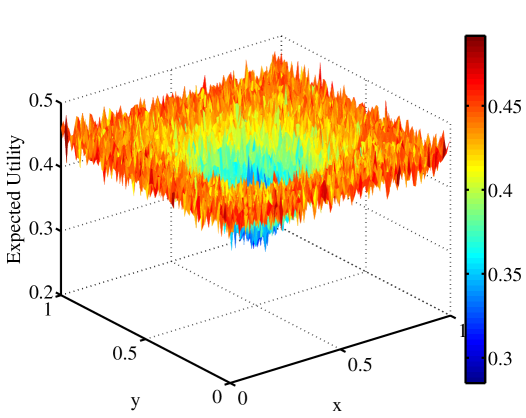
(a) $N=1001$, $M=2$

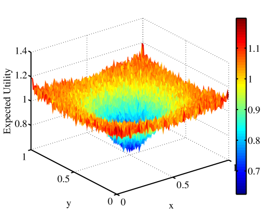
(b) $N=1001$, $M=11$

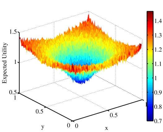
(c) $N=1001$, $M=101$

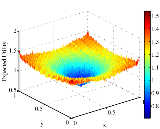
(d) $N=1001$, $M=1001$

Figure 2: Surface plots of independent $\hat{U}_{N,M}$ realizations, evaluated over the entire design space $[0,1]^{2}\ni\mathbf{d}=(x,y)$. Note that the vertical axis ranges and color scales vary among the subfigures.

where $\mathcal{H}_{s}\times\mathcal{Y}_{s}$ is the support of the joint density $f_{\bm{\Theta}_{s},\mathbf{Y}_{s}|\mathbf{d}}(\bm{\theta}_{s},\mathbf{y}_{s}|\mathbf{d})$. Our original estimator $\hat{U}_{N,M}$ is now unbiased for the new objective $\bar{U}_{M}$ by construction! The tradeoff, of course, is that the function being optimized is no longer the true $U$. But it is consistent in that $\bar{U}_{M}(\mathbf{d})\to U(\mathbf{d})$ as $M\to\infty$, for any $N>0$. (To illustrate this convergence, realizations of $\hat{U}_{N,M}$, i.e., Monte Carlo approximations of $\bar{U}_{M}$, are plotted in Figure 2 for varying $M$.)

The second requirement of IPA comprises conditions allowing an unbiased gradient estimator to be constructed by taking the gradient of the unbiased function estimator. Standard conditions (see, for example, [67]) require that the random quantity (e.g., $\hat{U}_{N,M}$) be almost surely continuous and differentiable. Here, because $\hat{U}_{N,M}$ is parameterized by continuous random variables that have densities with respect to Lebesgue measure, we can take a perspective that relies on Leibniz’s rule with the following conditions:

1. $\hat{U}_{N,M}$ and $\nabla_{\mathbf{d}}\left(\hat{U}_{N,M}\right)$ are continuous over the product space of design variables and random variables, $\mathcal{D}\times\mathcal{H}_{s}\times\mathcal{Y}_{s}$;

2. the density of the “noise” random variable is independent of $\mathbf{d}$.

The first condition supports the interchange of differentiation and integration according to Leibniz’s rule. This condition might be difficult to verify in arbitrary cases, but the use of finite-order polynomial forward models and continuous distributions for the prior and observational noise ensures that we meet the requirement.

The second condition is needed to preserve the form of the expectation. If it is violated, differentiation with respect to $\mathbf{d}$ must be performed on the $f_{\bm{\Theta}_{s},\mathbf{Y}_{s}|\mathbf{d}}(\bm{\theta}_{s},\mathbf{y}_{s}|\mathbf{d})$ term as well via the product rule, in which case the additional term $\int_{\mathcal{Y}_{s}}\int_{\mathcal{H}_{s}}\hat{U}_{N,M}(\mathbf{d},\bm{\theta}_{s},\mathbf{y}_{s})\,\nabla\left[f_{\bm{\Theta}_{s},\mathbf{Y}_{s}|\mathbf{d}}(\bm{\theta}_{s},\mathbf{y}_{s}|\mathbf{d})\right]\,d\bm{\theta}_{s}\,d\mathbf{y}_{s}$ would no longer be an expectation with respect to the original density. The likelihood-ratio method may be used to restore the expectation [68, 67], but it is not pursued here. Instead, it is simpler to transform the noise to a design-independent random variable as described in Section 2.2.2.

In the context of optimal Bayesian experimental design, the outcome of the experiment $\mathbf{Y}$ is a stochastic quantity that depends on the design $\mathbf{d}$. From the stochastic optimization perspective, $\mathbf{Y}$ is thus a noise variable. To demonstrate the transformation to design-independent noise, we assume a likelihood where the data result from an additive Gaussian perturbation to the forward model:

$$\mathbf{Y} = \mathbf{G}(\bm{\Theta},\mathbf{d})+\mathbf{E}$$ (16)

$$= \mathbf{G}(\bm{\Theta},\mathbf{d})+\mathbf{C}(\bm{\Theta},\mathbf{d})\mathbf{Z}.$$

Here $\mathbf{C}$ is a diagonal matrix with non-zero entries reflecting the dependence of the noise standard deviation on other quantities, and $\mathbf{Z}$ is a vector of i.i.d. standard normal random variables. For example, “10% Gaussian noise on the $c$th component” would translate to $C_{c,i}=\delta_{ci}0.1|G_{c}(\bm{\Theta},\mathbf{d})|$, where $\delta_{ci}$ is the Kronecker delta function. For other forms of the likelihood, the right-hand side of (16) is simply replaced by a generic function of $\bm{\Theta}$, $\mathbf{d}$, and some random variable $\mathbf{Z}$. Here, however, we will focus on the additive Gaussian form in order to derive illustrative expressions.

By extracting a design-independent random variable $\mathbf{Z}$ from the noise term $\mathbf{E}\equiv\mathbf{C}(\bm{\Theta},\mathbf{d})\mathbf{Z}$, we will satisfy the second condition above. The design-dependence of $\mathbf{Y}$ is incorporated into $\hat{U}_{N,M}$ by substituting (16) into (3):

$$\hat{U}_{N,M}(\mathbf{d},\bm{\theta}_{s},\mathbf{z}_{s}) = \frac{1}{N}\sum_{i=1}^{N}\left\{\ln\left[f_{\mathbf{Y}|\bm{\Theta},\mathbf{d}}\left(\left.\mathbf{G}(\bm{\theta}^{(i)},\mathbf{d})+\mathbf{C}(\bm{\theta}^{(i)},\mathbf{d})\mathbf{z}^{(i)}\right|\bm{\theta}^{(i)},\mathbf{d}\right)\right]\right.$$ (17)

$$-\left.\ln\left[\frac{1}{M}\sum_{j=1}^{M}f_{\mathbf{Y}|\bm{\Theta},\mathbf{d}}\left(\left.\mathbf{G}(\bm{\theta}^{(i)},\mathbf{d})+\mathbf{C}(\bm{\theta}^{(i)},\mathbf{d})\mathbf{z}^{(i)}\right|\bm{\theta}^{(i,j)},\mathbf{d}\right)\right]\right\},$$

where $\mathbf{z}_{s}=\left\{\mathbf{z}^{(i)}\right\}$. The new noise variables are now independent of $\mathbf{d}$. The samples of $\mathbf{y}^{(i)}$ drawn from the likelihood are instead realized by drawing $\mathbf{z}^{(i)}$ from $N(\mathbf{0},\mathbf{I})$, then multiplying these samples by $\mathbf{C}$ and adding them to the model output.

With all conditions for IPA satisfied, an unbiased estimator of the gradient of $\bar{U}_{M}$, corresponding to $\hat{g}$ in (6), is simply $\nabla_{\mathbf{d}}\hat{U}_{N,M}(\mathbf{d},\bm{\theta}_{s},\mathbf{z}_{s})$ since

$$\mathbb{E}_{\bm{\Theta}_{s},\mathbf{Z}_{s}}\left[\nabla_{\mathbf{d}}\hat{U}_{N,M}(\mathbf{d},\bm{\Theta}_{s},\mathbf{Z}_{s})\right] = \int_{\mathcal{Z}_{s}}\int_{\bm{\Theta}_{s}}\nabla_{\mathbf{d}}\hat{U}_{N,M}(\mathbf{d},\bm{\theta}_{s},\mathbf{z}_{s})f_{\bm{\Theta}_{s},\mathbf{Z}_{s}}(\bm{\theta}_{s},\mathbf{z}_{s})\,d\bm{\theta}_{s}\,d\mathbf{z}_{s}$$ (18)

$$= \nabla_{\mathbf{d}}\int_{\mathcal{Z}_{s}}\int_{\bm{\Theta}_{s}}\hat{U}_{N,M}(\mathbf{d},\bm{\theta}_{s},\mathbf{z}_{s})f_{\bm{\Theta}_{s},\mathbf{Z}_{s}}(\bm{\theta}_{s},\mathbf{z}_{s})\,d\bm{\theta}_{s}\,d\mathbf{z}_{s}$$

$$= \nabla_{\mathbf{d}}\mathbb{E}_{\bm{\Theta}_{s},\mathbf{Z}_{s}}\left[\hat{U}_{N,M}(\mathbf{d},\bm{\Theta}_{s},\mathbf{Z}_{s})\right]$$

$$= \nabla_{\mathbf{d}}\bar{U}_{M}(\mathbf{d}),$$

where $\mathcal{Z}_{s}$ is the support of $f_{\mathbf{Z}_{s}}(\mathbf{z}_{s})$. This gradient estimator is therefore suitable for use in RM.

The gradient of the finite-sample Monte Carlo approximation of $U(\mathbf{d})$, i.e., $\nabla\hat{h}_{N,M}(\cdot,w_{s}^{t})$ used in SAA, takes exactly the same form. The only difference between the two is that $\hat{g}$ lets $\bm{\Theta}_{s}$ and $\mathbf{Z}_{s}$ be random at every iteration of the optimization process. When used as $\nabla\hat{h}_{N,M}(\cdot,w_{s}^{t})$, $\bm{\Theta}_{s}$ and $\mathbf{Z}_{s}$ are frozen at some realization throughout the optimization process. In either case, these gradient expressions contain derivatives of the likelihood function and thus derivatives $\nabla_{\mathbf{d}}\mathbf{G}(\bm{\theta},\mathbf{d})$. When $\mathbf{G}$ is replaced with a polynomial expansion, these derivatives can be computed inexpensively. Detailed derivations of the gradient estimator using orthogonal polynomial expansions can be found in the Appendix.

5 Source Inversion Problem

5.1 Governing equations

We demonstrate the optimal Bayesian experimental design formulation and our stochastic optimization tools on a two-dimensional contaminant identification problem. The goal is to place a single sensor that yields maximum information about the location of the contaminant source. Contaminant transport is governed by a scalar diffusion equation on a square domain:

$$\frac{\partial w}{\partial t}=\nabla^{2}w+S\left(\mathbf{x}_{\mathrm{src}},\mathbf{x},t\right),\qquad\mathbf{x}\in\mathcal{X}=\left[0,1\right]^{2},$$ (19)

where $w(\mathbf{x},t;\mathbf{x}_{\mathrm{src}})$ is the space-time concentration field parameterized by the coordinate of the source center $\mathbf{x}_{\mathrm{src}}$. We impose homogeneous Neumann boundary conditions

$$\nabla w\cdot\mathbf{n}=0\qquad\textrm{ on }\partial\mathcal{X},$$ (20)

along with a zero initial condition

$$w(\mathbf{x},0;\mathbf{x}_{\mathrm{src}})=0.$$ (21)

The source function has a Gaussian spatial profile

$$S\left(\mathbf{x}_{\mathrm{src}},\mathbf{x},t\right)=\left\{\begin{array}[]{cc}\frac{s}{2\pi h^{2}}\exp\left(-\frac{\|\mathbf{x}_{\mathrm{src}}-\mathbf{x}\|^{2}}{2h^{2}}\right),&0\leq t<\tau\\ 0,&t\geq\tau\end{array}\right.$$ (24)

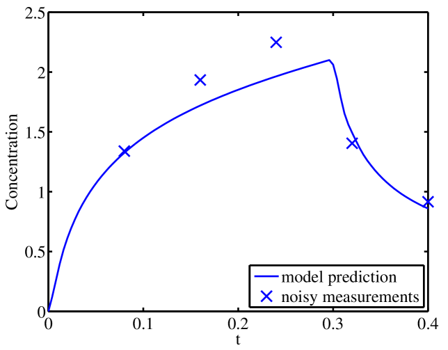
Figure 1: Example forward model solution and realizations from the likelihood. In particular, the solid line represents the time-dependent contaminant concentration $w(\mathbf{x},t;\mathbf{x}_{\mathrm{src}})$ at $\mathbf{x}=\mathbf{x}_{\mathrm{sensor}}=(0.0,0.0)$, given a source centered at $\mathbf{x}_{\mathrm{src}}=(0.1,0.1)$, source strength $s=2.0$, width $h=0.05$, and shutoff time $\tau=0.3$. Parameters are defined in the diffusion equation (19). The five crosses represent noisy measurements at five designated measurement times.

where $s$, $h$, and $\tau$ are known (prescribed) source intensity, width, and shutoff time parameters, respectively, and $\mathbf{x}_{\mathrm{src}}\equiv\left(\Theta_{x},\Theta_{y}\right)$ is the unknown source location that we would ultimately like to infer. The design variable is the location of a single sensor, $\mathbf{x}_{\mathrm{sensor}}\equiv\left(d_{x},d_{y}\right)$, and the measurement data $\{Y_{i}\}_{i=1}^{5}$ comprise five noisy point observations of $w$ at the sensor location and at five equally-spaced sample times. For this study, we choose $s=2.0$, $h=0.05$, $\tau=0.3$; a uniform prior $\Theta_{x},\Theta_{y}\sim\mathcal{U}\left(0,1\right)$; and an additive error model $Y_{i}=w\left(\mathbf{x}_{\mathrm{sensor}},t_{i},;\mathbf{x}_{\mathrm{src}}\right)+E_{i},i=1\ldots 5$, such that the $E_{i}$ are zero-mean Gaussian random variables, mutually independent given $\mathbf{x}_{\mathrm{sensor}}$ and $\mathbf{x}_{\mathrm{src}}$, each with standard deviation $\sigma_{i}=0.1+0.1\left|w\left(\mathbf{x}_{\mathrm{sensor}},t_{i};\mathbf{x}_{\mathrm{src}}\right)\right|$. In other words, the error associated with the data has a “floor” value of 0.1 plus an additional contribution that is 10% of the signal. The sensor may be placed anywhere in the square domain, such that the design space is $\left(d_{x},d_{y}\right)\in[0,1]^{2}$. Figure 1 shows an example concentration profile and measurements.

Evaluating the forward model thus requires solving the partial differential equation (19) at fixed realizations of $\bm{\theta}=\mathbf{x}_{\mathrm{src}}$ and extracting the solution field at the design location $\mathbf{d}=\mathbf{x}_{\mathrm{sensor}}$. We discretize (19) using 2nd-order centered differences on a 25 $\times$ 25 spatial grid and a 4th-order backward differentiation formula for time integration. As described in Section 3, we replace the full forward model with a polynomial chaos surrogate, for computational efficiency. To this end, we construct a Legendre polynomial approximation of the forward model output over the 4-dimensional joint parameter and design space, using a total-order polynomial truncation of degree $12$ and $10^{6}$ forward model evaluations. This high polynomial degree and rather large number of forward model evaluations were deliberately selected in order to render truncation and aliasing error insignificant in our study. Optimal experimental design results of similar quality may be obtained for this problem with surrogates of lower order and with far fewer quadrature points (e.g., degree 4 with $10^{4}$ forward model evaluations) but for brevity they are not included here. The relative $L^{2}$ errors of the current surrogate range from $6\times 10^{-3}$ to $10^{-6}$.

The optimal Bayesian experimental design formulation now seeks the sensor location $\mathbf{x}^{*}_{\mathrm{sensor}}$ such that when the experiment is performed, on average—i.e., averaged over all possible source locations according to the prior, and over all possible resulting concentration measurements according to the likelihood—the five concentration readings $\left\{Y_{i}\right\}_{i=1}^{5}$ yield the greatest information gain from prior to posterior.

5.2 Results

5.2.1 Objective function

Before we present the results of numerical optimization, we first explore the properties of the expected information gain objective. Numerical realizations of $\hat{U}_{N,M}$ for $N=1001$ and $M=2$, 11, 101, and 1001 are shown in Figure 2. These plots can be interpreted as 1-sample Monte Carlo approximations of $\bar{U}_{M}=\mathbb{E}[\hat{U}_{N,M}]$, or equivalently, as $l$-sample Monte Carlo approximations of $\bar{U}_{M}=\mathbb{E}[\hat{U}_{(N/l),M}]$. As $N$ grows, $\hat{U}_{N,M}$ becomes a better approximation to $\bar{U}_{M}$ and as $M$ grows, $\bar{U}_{M}$ becomes a better approximation to $U$. The figures show that values of $\hat{U}_{N,M}$ increase when $M$ increases (for fixed $N$), suggesting a negative bias at finite $M$. At the same time, the objective becomes less flat in $\mathbf{d}$; since $U$ is certainly closer to the $M=1001$ surface than the $M=2$ surface, these results suggest that $U$ is not particularly flat in $\mathbf{d}$. This feature of the current design problem is encouraging, since stochastic optimization problems with higher curvature can be more easily solved; in the context of SA, for example, they effectively have a higher signal-to-noise ratio.

The expected information gain objective inherits symmetries from the square, as expected from the physical nature of the problem. The plots also suggest a smooth albeit nonconvex underlying objective $U$, with inflection points lying on an interior circle and four local maxima symmetrically located at the corners of the design space. The best placement for a single sensor is therefore at the corners of the design space, while the worst placement is at the center. The reason for this perhaps counterintuitive result is that the diffusion process is isotropic: a series of concentration measurements can only determine the distance of the source from the sensor, not its orientation. The posterior distribution thus resembles an annulus of constant radius surrounding the sensor. A sensor placement that minimizes the area of these annuli, averaged over all possible source locations according to the prior, tends to be optimal. In this problem, because of the domain geometry and the magnitude of the observational noise, these optimal locations happen to be the furthest points from the domain center, i.e., the corners.

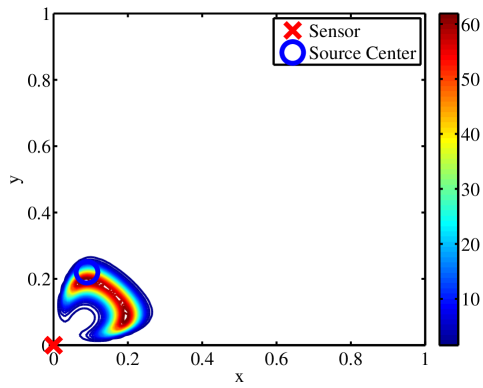
(a) $\mathbf{x}_{\mathrm{sensor}}=(0.0,0.0)$

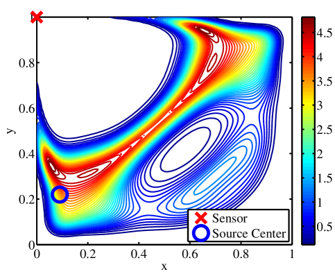
(b) $\mathbf{x}_{\mathrm{sensor}}=(0.0,1.0)$

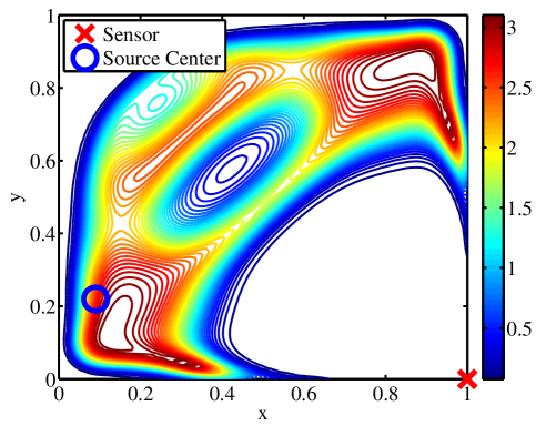
(c) $\mathbf{x}_{\mathrm{sensor}}=(1.0,0.0)$

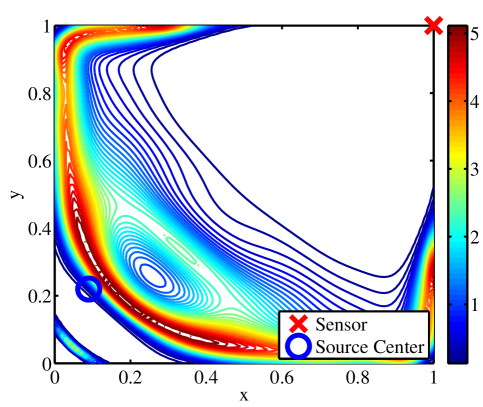
(d) $\mathbf{x}_{\mathrm{sensor}}=(1.0,1.0)$

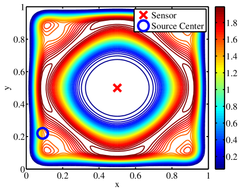
(e) $\mathbf{x}_{\mathrm{sensor}}=(0.5,0.5)$

Figure 3: Contours of posterior probability density for the source location, given different sensor placements. The true source location, marked with a blue circle, is $\mathbf{x}_{\mathrm{src}}=(0.09,0.22)$.

Figure 3 shows posterior probability densities for the source location, under different sensor placements, given data generated from a “true” source centered at $\mathbf{x}_{\mathrm{src}}=(0.09,0.22)$. The posterior densities are evaluated using the polynomial chaos surrogate, while the data are generated by directly solving the diffusion equation on a denser (101 $\times$ 101) spatial grid than before and then adding the Gaussian noise described in Section 5.1. Note that the posteriors are extremely non-Gaussian. Moreover, they generally include the true source location, but do not center on it. Reasons for not expecting the posterior mode to match the true source location are twofold: first, we have only 5 measurements, each perturbed with a relatively significant random noise; second, there is model error, due to mismatch between the polynomial chaos approximation constructed from the coarser spatial discretization of the PDE and the more finely discretized PDE model used to simulate the data.^, For this source configuration, it appears that a sensor placed at any of the corners yields a “tighter” posterior than a sensor placed at the center. But we must keep in mind that this result is not guaranteed for all source locations and data realizations; it depends on where the source actually is. [Imagine, for example, if the source happened to be very close to the center of the domain; then the sensor at (0.5, 0.5) would yield the tightest posterior.] What the optimal experimental design method yields is the optimal sensor placement averaged over the prior distribution of the source location and the predictive distribution of the data.

5.2.2 Stochastic optimization results

We now analyze the optimization results, first assessing the behavior of the two stochastic optimization methods individually, and then comparing their performance.

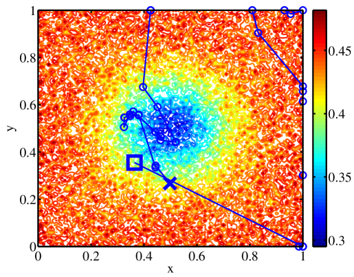
(a) $N=1$, $M=2$

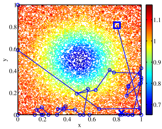
(b) $N=1$, $M=11$

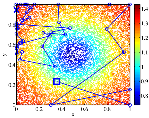
(c) $N=1$, $M=101$

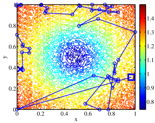
(d) $N=1$, $M=1001$

Figure 4: Sample paths of the RM algorithm with $N=1$, overlaid on $\hat{U}_{N,M}$ surfaces from Figure 2 with the corresponding $M$ values. The large $\square$ is the starting position and the large $\times$ is the final position.

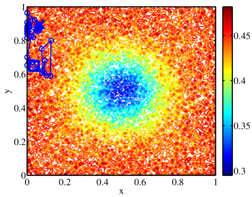
(a) $N=11$, $M=2$

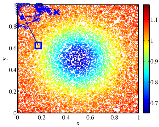
(b) $N=11$, $M=11$

(c) $N=11$, $M=101$

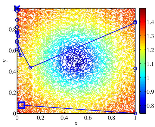
(d) $N=11$, $M=1001$

Figure 5: Sample paths of the RM algorithm with $N=11$, overlaid on $\hat{U}_{N,M}$ surfaces from Figure 2 with the corresponding $M$ values. The large $\square$ is the starting position and the large $\times$ is the final position.

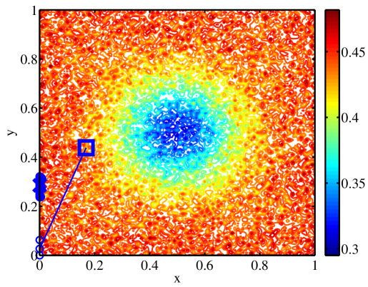
(a) $N=101$, $M=2$

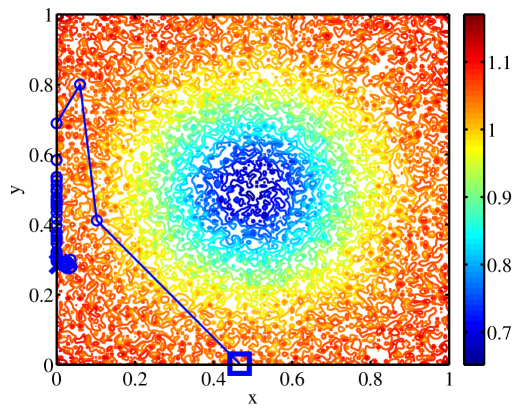
(b) $N=101$, $M=11$

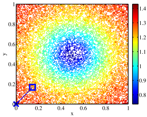
(c) $N=101$, $M=101$

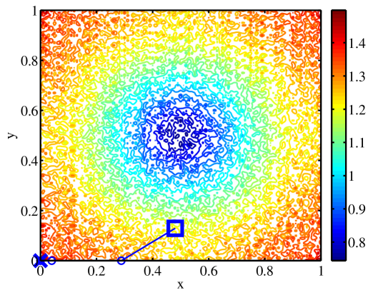
(d) $N=101$, $M=1001$

Figure 6: Sample paths of the RM algorithm with $N=101$, overlaid on $\hat{U}_{N,M}$ surfaces from Figure 2 with the corresponding $M$ values. The large $\square$ is the starting position and the large $\times$ is the final position.

Recall that the RM algorithm is essentially a steepest-ascent method (since we are maximizing the objective) with a stochastic gradient estimate. Figures 4–6 each show four sample RM optimization paths overlaid on the $\hat{U}_{N,M}$ surfaces from Figure 2. The optimization does not always proceed in an ascent direction, due to the noise in the gradient estimate, but even a noisy gradient can be useful in eventually guiding the algorithm to regions of high objective value. Naturally, fewer iterations are needed and good designs are more likely to be found when the variance of the gradient estimator is reduced by increasing $N$ and $M$. Note that one must be cautious not to over-generalize from these figures, since the paths shown in each plot are not necessarily representative. Instead, their purpose is to provide intuition about the optimization mechanics. Data derived from many runs are more appropriate performance metrics, and will be used later in this section.

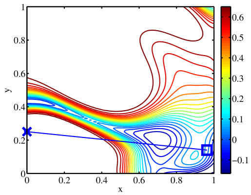
(a) $N=1$, $M=2$

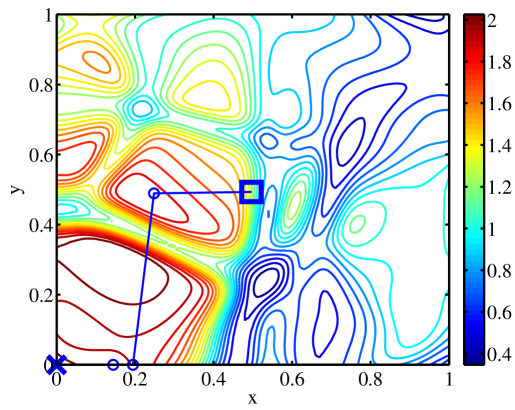
(b) $N=1$, $M=11$

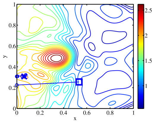
(c) $N=1$, $M=101$

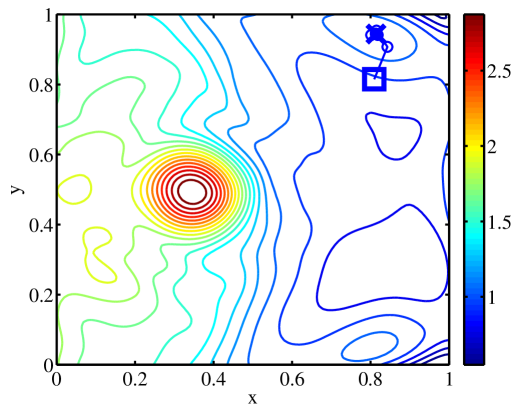
(d) $N=1$, $M=1001$

Figure 7: Realizations of the objective function surface using SAA, and corresponding steps of BFGS, with $N=1$. The large $\square$ is the starting position and the large $\times$ is the final position.

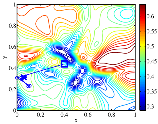
(a) $N=11$, $M=2$

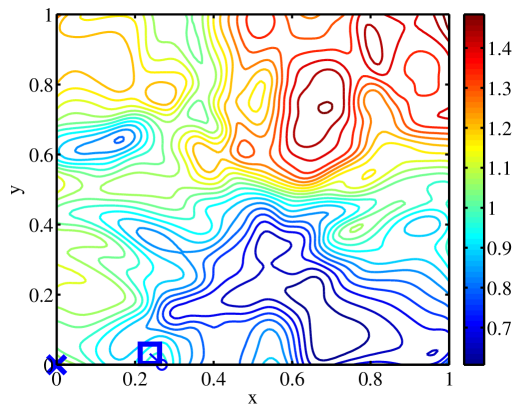
(b) $N=11$, $M=11$

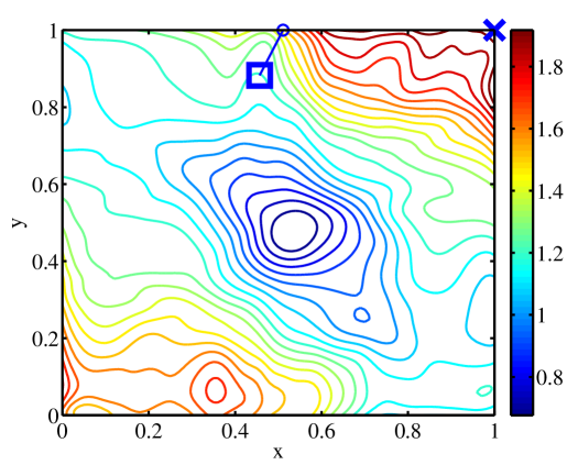
(c) $N=11$, $M=101$

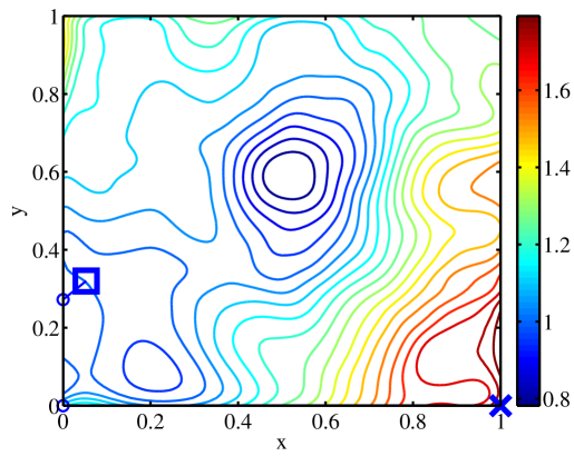
(d) $N=11$, $M=1001$

Figure 8: Realizations of the objective function surface using SAA, and corresponding steps of BFGS, with $N=11$. The large $\square$ is the starting position and the large $\times$ is the final position.

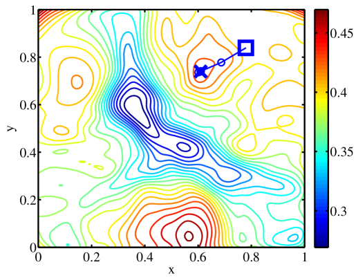
(a) $N=101$, $M=2$

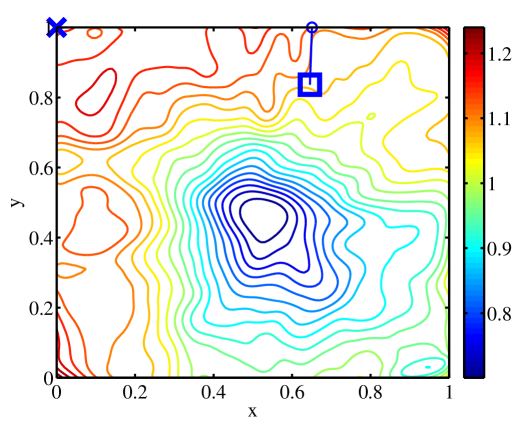
(b) $N=101$, $M=11$

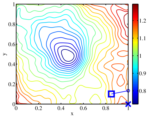
(c) $N=101$, $M=101$

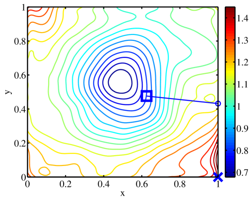
(d) $N=101$, $M=1001$

Figure 9: Realizations of the objective function surface using SAA, and corresponding steps of BFGS, with $N=101$. The large $\square$ is the starting position and the large $\times$ is the final position.

For SAA-BFGS, each choice of the sample set $w_{x}^{t}$ yields a different deterministic objective; example realizations of this objective surface are shown in Figures 7–9. For each realization, a local maximum is found efficiently by the BFGS algorithm, requiring only a few (usually less than 10) iterations. For each set of results corresponding to a particular $N$ (i.e., each of Figures 7–9), the random numbers used for smaller values of $M$ are proper subsets of those used for larger $M$. We thus expect some similarity and a sense of convergence among the subplots in each figure. Note also that when $N$ is low, realizations of the objective can be extremely different from Figure 2 (for example, the plots in Figure 7 have local maxima near the center of the domain), although improvement is observed as $N$ is increased. In general, each deterministic problem in SAA can have very different features than the underlying objective function. None of the realizations encountered here has maxima at the corners, or is even symmetric. Nonetheless, when sampling over many SAA subproblems, even a low $N$ can provide reasonably good results. This will be shown in Tables 1 and 2, and discussed in detail below.

To compare the performance of RM and SAA-BFGS, 1000 independent runs are conducted for each algorithm, over a matrix of $N$ and $M$ values. The starting locations of these runs are sampled from a uniform distribution over the design space. We make reasonable choices for the numerical parameters in each algorithm (e.g., gain schedule scaling, termination criteria) leading to similar run times. Histograms of the final design parameters (sensor positions) resulting from each set of 1000 optimization runs are shown in Table 1. The top figures in each major row represent RM results, while the bottom figures in each major row correspond to SAA-BFGS results. Columns correspond to different values of $M$. It is immediately apparent that more designs cluster at the corners of the domain as $N$ and $M$ are increased. For the case with the largest number of samples ($N=101$ and $M=1001$), each corner has around 250 designs, suggesting that higher sample sizes cannot further improve the optimization results. An “overlap” in quality across the different $N$ cases is also observed: for example, results of the $N=101$, $M=2$ case are worse than those of the $N=11$, $M=1001$ case. A balance is thus needed in choosing samples sizes $N$ and $M$, and it is not ideal to heavily favor sampling either the inner or outer Monte Carlo loop in $\hat{U}_{N,M}$. Overall, comparing the RM and SAA-BFGS plots at intermediate values of $M$ and $N$, we see that RM has a slight advantage over SAA-BFGS by placing more designs at the corners.

The distribution of final designs alone does not reflect the robustness of the optimization results. For example, if $U$ is very flat near the optimum, then suboptimal designs need not be very close to the true optimum in the design space to be considered good designs in practice. To evaluate robustness, a “high-quality” objective estimate $\hat{U}_{1001,1001}$ is computed for each of the 1000 final designs considered above. The resulting histograms are shown in Table 2, where again the top subrows are for RM and the bottom subrows are for SAA-BFGS, with the results covering a full range of $N$ and $M$ values. In keeping with our previous observations, performance is improved as $N$ and $M$ are increased—in that the mean (over the optimization runs) expected information gain increases, while the variance in the expected information gain decreases. Note, however, that even if all 1000 optimization runs produced identical final designs, this variance will not reach zero, as there exists a “floor” corresponding to the variance of the estimator $\hat{U}_{1001,1001}$. This minimum variance can be observed in the histograms of the RM results with $N=101$ and $M=101$ or $1001$.

One interesting feature of the histograms in Table 2 is their bimodality. The higher mode reflects designs near the four corners, while the lower mode encompasses all other suboptimal designs. As $N$ or $M$ increase, we observe a transfer of probability mass from the lower mode to the upper mode. However, the sample sizes are not large enough for the lower mode to completely disappear for most cases; it is only absent in the two RM cases with the largest sample sizes. Overall, the histograms are similar in shape for both algorithms, but RM appears to produce less variability in the expected information gain, particularly at high $N$ values.

Table 3 shows histograms of optimality gap estimates from the 1000 SAA-BFGS runs. Since we are dealing with a maximization problem (for the expected information gain), the estimator from §2.2.2 is reversed in sign, such that the upper bound is now $\bar{h}_{N}$ and the lower bound is $\hat{h}_{N^{\prime}}(\hat{x}_{s}^{t},w_{s^{\prime}}^{t})$. The lower bound must be evaluated with the same inner-loop Monte Carlo sample size $M$ used in the optimization run in order to represent an identically-biased underlying objective; hence, the lower bound values will not be the same as the “high-quality” objective estimates $\hat{U}_{1001,1001}$ discussed above. From the table, we observe that as $N$ increases, values of the optimality gap estimate decrease. This is a result of the lower bound rising with $N$ (since the optimization is better able to find designs in regions of large $\bar{U}_{M}$, e.g., corners of the domains in Table 1), and the upper bound simultaneously falling (since its positive bias monotonically decreases with $N$ [39]). Consequently, both bounds become tighter and the gap estimates tend toward zero. As $M$ increases, the variance of the gap estimates increases. Since the upper bound ($\bar{h}_{N}$) is fixed for a given set of SAA runs, the spread is only affected by the variability of the lower bound. Indeed, from Figure 2, it is apparent that the objective becomes less flat as $M$ increases, with the highest gradients (considering the good design regions only) occurring at the corners. This translates to a higher sensitivity, as a small “imperfection” in the design would lead to larger changes in objective estimate; one then would expect the variation of $\hat{h}_{N^{\prime}}(\hat{x}_{s}^{t},w_{s^{\prime}}^{t})$ to become higher as well, leading to greater variance in the gap estimates. Finally, as $M$ increases, the histogram values tend to increase, but they increase more slowly for larger values of $N$. Some intuition for this result may be obtained by considering the relative rates of change of the upper and lower bounds with respect to $M$, given different values of $N$. Again referring to Figure 2, the objective values generally increase with $M$, indicating an increase of the lower bound. This increase should be more pronounced for larger $N$, since the optimization converges to designs closer to the corners, where, as mentioned earlier, the objective has larger gradient. The upper bound increases with $M$ as well, as indicated by the contour levels in Figures 7–9. But this rate of increase is observed to be slowest at the highest $N$ (i.e., in Figure 9). Combining these two effects, it is reasonable that as $N$ increases, the gap estimate will increase with $M$ at a slower rate.

Can the optimality gap be used to choose values of $M$ and $N$? For a fixed $M$, we certainly have convergence as $N$ increases, and the gap estimate can be a good indicator of solution quality. However, because different values of $M$ correspond to different objective surfaces (due to the bias of $\hat{U}_{N,M}$), the optimality gap is unsuitable for comparisons across different values of $M$; indeed, in our example, even though solution quality is improved with $M$, the gap estimates appear looser and noisier.

Another performance metric we extract from the stochastic optimization runs is the number of iterations required to reach a solution; histograms of iteration number for RM and SAA, for the same matrix of $M$ and $N$ values, are shown in Table 4. At low sample sizes, many of the SAA-BFGS runs take only a few iterations, while almost all of the RM runs terminate at the maximum allowable number of iterations (50 in this case). This difference again reflects the efficiency of BFGS for deterministic optimization problems. As $N$ and $M$ are increased, the histograms show a “transfer of mass” from higher iteration numbers to lower iteration numbers, coinciding somewhat with the bimodal behavior described previously. The reduction in iteration number with increased sample size implies that an $n-$fold increase in sample size leads to an increase in computational time that is often much less than a factor of $n$. Accounting for this sublinear relationship when allocating computational resources, especially if samples can be drawn in parallel, can lead to substantial savings. Although SAA-BFGS generally requires fewer iterations, each iteration takes longer than a step of RM. RM thus offers a higher “resolution” in run times, potentially giving more freedom to the user in stopping the algorithm. RM thus becomes more attractive as the evaluation of the objective function becomes more expensive.

As a single integrated measure of the quality of the stochastic optimization solutions, we evaluate the following mean square error (MSE):

$$\mathrm{MSE}=\frac{1}{T}\sum_{t=1}^{T}\left(\hat{U}_{1001,1001}(\mathbf{d}^{t},\bm{\theta}_{s^{\prime}}^{t},\mathbf{z}_{s^{\prime}}^{t})-U^{\mathrm{ref}}\right)^{2},$$ (25)

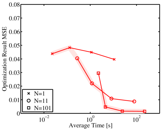
(a) RM

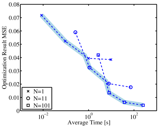
(b) SAA-BFGS

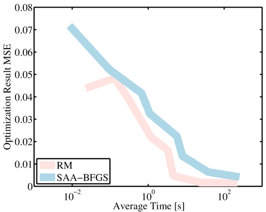
(c) RM and SAA-BFGS “optimal fronts”

Figure 10: Mean square error, defined in (25), versus average run time for each optimization algorithm and various choices of inner-loop and outer-loop sample sizes. The highlighted curves are “optimal fronts” for RM (light red) and SAA-BFGS (light blue).

where $\mathbf{d}^{t}$, $t=1\ldots T$, are the final designs from a given optimization algorithm, and $U^{\mathrm{ref}}$ is the true optimal value of the expected information gain. Since the true optimum is unavailable in this study, $U^{\mathrm{ref}}$ is taken to be the maximum value of the objective over all runs. Recall that the MSE combines the effects of bias and variance; here it reflects the variance in objective values plus the difference (squared) between the mean objective value and the true optimum, calculated via $T=1000$ replicated optimization runs. Figure 10 relates solution quality to computational effort by plotting the MSE against average computational time (per run). Each symbol represents a particular value of $N$ ($\times$, $\bigcirc$, and $\square$ represent $N=1$, 11, and 101, respectively), while the four different $M$ values are reflected through the average run times. These plots confirm the behavior we have previously encountered. Solution quality generally improves (lower MSE) with increasing sample sizes, although a balanced allocation of samples must be chosen. For instance, a large $N$ with small $M$ can yield inferior solutions to a smaller $N$ with larger $M$; while, for any given $N$, continued increases in $M$ beyond some threshold yield minimal improvements in MSE. The best sample allocation is described by the minimum of all the curves. We highlight these “optimal fronts” in light red for RM and in light blue for SAA-BFGS. Monte Carlo error in the “high-quality” estimator $\hat{U}_{1001,1001}$ may also be reflected in the non-zero MSE asymptote for the high-$N$ RM cases.

According to Figure 10, RM outperforms SAA-BFGS by consistently achieving smaller MSE for a given computational effort. One should be cautious, however, in generalizing from these numerical experiments. The advantage of RM is relatively small, and other factors such as code optimization, choices of algorithm parameters, and of course the experimental design problem itself can affect or even reverse this advantage.

6 Conclusions

This paper has explored the stochastic optimization problem arising from a general nonlinear formulation of optimal Bayesian experimental design. In particular, we employed an objective that reflects the expected information gain in model parameters due to an experiment, and formulated two gradient-based approaches to stochastic optimization in this context: Robbins-Monro (RM) stochastic approximation, and sample average approximation (SAA) coupled with BFGS. Both of these algorithms require gradient information derived from Monte Carlo approximations of the objective: an unbiased gradient estimator in the former case, and gradients of a finite-sample Monte Carlo estimate in the latter case. Methods for extracting this gradient information must contend with an estimator of expected information gain that is not a simple Monte Carlo sum, but rather contains nested Monte Carlo estimates. It is therefore expensive to evaluate, and biased for finite inner-loop sample sizes. To circumvent these challenges, we approximate the forward model embedded in the likelihood function with a polynomial chaos expansion, and maximize the expected information gain computed via this approximation instead. Gradient information is readily extracted from the polynomial chaos expansion, with the help of a simple perturbation analysis.

We analyze the performance of the two stochastic optimization approaches using the problem of sensor placement for source inversion, cast as optimal experimental design over a continuous design space. Numerical experiments, performed over a matrix of inner- and outer-loop sample sizes, examine the impact of bias and variance in the objective function and gradient estimates on the efficiency of the optimization algorithms and on the quality of the resulting solutions. These experiments suggest (unsurprisingly) that solution quality improves as sample sizes increase, but also that optimization runs may converge in fewer iterations for larger sample sizes. Also, a balanced allocation of computational resources between the inner and outer Monte Carlo sums is important for computational efficiency. Arbitrarily increasing the inner-loop sample size, for instance, yields little improvement in solution quality when the outer-loop samples are too few. Our results also suggest that RM has a consistent performance advantage over SAA-BFGS, but this conclusion is necessarily problem-dependent. Instead of declaring one algorithm to be superior, our broader goal is to illustrate the differences between the two algorithms and provide some selection guidelines based on their properties.

The SAA approach may provide more flexibility than SA, as it can be combined with any deterministic optimization algorithm, whereas the SA approach essentially specifies the form of each optimization iteration. SAA’s flexibility allows one to take advantage of problem structure: if realizations of the objective surface are known to be “well-behaved” and smooth, gradient-based algorithms such as BFGS can exploit this regularity, as in the present source inversion example. On the other hand, if the objective is not smooth, or if gradients are not available, some gradient-free deterministic algorithm may be more appropriate. Estimates of optimality gap, obtained from replicate SAA solutions, can be used to adaptively adjust the outer-loop Monte Carlo sample size, but are unsuitable for assessing the inner-loop sample size because of bias effects. Future work could employ the common random number stream approach in [40] to obtain a lower-variance estimate of optimality gap (along with a confidence interval), or the jackknife technique proposed in [69] for bias reduction.

The RM algorithm and other stochastic approximation methods must use a stochastic gradient estimator. This can lead to poor performance if only high-variance gradient estimates are available. In the current context, increasing the outer-loop sample size reduces variance and the RM algorithm performed relatively well. Note that the frequent (yet cheaper) steps of RM effectively provide a finer resolution in run time than SAA, giving the user more freedom to terminate the algorithm without losing much progress between the termination time and the previous optimization iteration. Therefore, RM may become more attractive as objective evaluations become more expensive.

The present approach used a global polynomial chaos surrogate, constructed over the product of the parameter space $\mathcal{H}$ and the design space $\mathcal{D}$. In model-based methods for deterministic derivative-free optimization, one might prefer to construct local surrogates valid over increasingly smaller intervals of $\mathcal{D}$, particularly as one approaches the optimum. Pursuing similar ideas in the stochastic context could possibly offer additional accuracy, but sampling errors in the stochastic optimization solution will always limit potential gains.

Finally, as we pointed out in Section 2.1, this paper has focused on batch or open-loop experimental design, where the parameters for all experiments are chosen before data are actually collected. An important target for future work is rigorous sequential or closed-loop design, where the data from one set of experiments are used to guide the choice of the next set. Here we expect stochastic optimization algorithms, for expected information gain and other objectives, to continue playing a crucial role.

7 Acknowledgements

This work was partially supported by the Computational Mathematics Program of the Air Force Office of Scientific Research and by the National Science Foundation under award number ECCS-1128147.

8 Figures and Tables

	2	11	101	1001
$1$
$11$
$101$

Table 1: Histograms of final search positions resulting from 1000 independent runs of RM (top subrows) and SAA (bottom subrows) over a matrix of $N$ and $M$ sample sizes. For each histogram, the bottom-right and bottom-left axes represent the sensor coordinates $x$ and $y$, respectively, while the vertical axis represents frequency.

	2	11	101	1001
1
11
101

Table 2: High-quality expected information gain estimates at the final sensor positions resulting from 1000 independent runs of RM (top subrows, blue) and SAA-BFGS (bottom subrows, red). For each histogram, the horizontal axis represents values of $\hat{U}_{M=1001,N=1001}$ and the vertical axis represents frequency.

	2	11	101	1001
1
11
101

Table 3: Histograms of optimality gap estimates for SAA-BFGS, over a matrix of samples sizes $M$ and $N$. For each histogram, the horizontal axis represents value of the gap estimate and the vertical axis represents frequency.

	2	11	101	1001
1
11
101

Table 4: Number of iterations in each independent run of RM (top subrows, blue) and SAA-BFGS (bottom subrows, red), over a matrix of sample sizes $M$ and $N$. For each histogram, the horizontal axis represents iteration number and the vertical axis represents frequency.

Appendix: Analytical Derivation of the Unbiased Gradient Estimator

In this section, we derive the analytical form of the unbiased gradient estimator $\nabla\hat{U}_{N,M}(\mathbf{d},\bm{\theta}_{s},\mathbf{z}_{s})$, following the method presented in Section 4.

The estimator $\hat{U}_{N,M}(\mathbf{d},\bm{\theta}_{s},\mathbf{z}_{s})$ is defined in (17). Its gradient in component form is

$$\nabla\hat{U}_{N,M}(\mathbf{d},\bm{\theta}_{s},\mathbf{z}_{s})=\left[\begin{array}[]{c}\frac{\partial}{\partial d_{1}}\hat{U}_{N,M}(\mathbf{d},\bm{\theta}_{s},\mathbf{z}_{s})\\ \frac{\partial}{\partial d_{2}}\hat{U}_{N,M}(\mathbf{d},\bm{\theta}_{s},\mathbf{z}_{s})\\ \vdots\\ \frac{\partial}{\partial d_{a}}\hat{U}_{N,M}(\mathbf{d},\bm{\theta}_{s},\mathbf{z}_{s})\\ \vdots\\ \frac{\partial}{\partial d_{n_{d}}}\hat{U}_{N,M}(\mathbf{d},\bm{\theta}_{s},\mathbf{z}_{s})\end{array}\right],$$ (32)

where $n_{d}$ is the dimension of the design parameters $\mathbf{d}$ and $d_{a}$ denotes the $a$th component of $\mathbf{d}$. The $a$th component of the gradient is then

$$\frac{\partial}{\partial d_{a}}\hat{U}_{N,M}(\mathbf{d},\bm{\theta}_{s},\mathbf{z}_{s}) = \frac{1}{N}\sum_{i=1}^{N}\left\{\frac{\frac{\partial}{\partial d_{a}}f_{\mathbf{Y}|\bm{\Theta},\mathbf{d}}\left(\mathbf{G}(\bm{\theta}^{(i)},\mathbf{d})+\mathbf{C}(\bm{\theta}^{(i)},\mathbf{d})\mathbf{z}^{(i)}\left|\bm{\theta}^{(i)},\mathbf{d}\right.\right)}{f_{\mathbf{Y}|\bm{\Theta},\mathbf{d}}\left(\mathbf{G}(\bm{\theta}^{(i)},\mathbf{d})+\mathbf{C}(\bm{\theta}^{(i)},\mathbf{d})\mathbf{z}^{(i)}\left|\bm{\theta}^{(i)},\mathbf{d}\right.\right)}\right.$$ (33)

$$\left.-\frac{\sum_{j=1}^{M}\frac{\partial}{\partial d_{a}}f_{\mathbf{Y}|\bm{\Theta},\mathbf{d}}\left(\mathbf{G}(\bm{\theta}^{(i)},\mathbf{d})+\mathbf{C}(\bm{\theta}^{(i)},\mathbf{d})\mathbf{z}^{(i)}\left|\bm{\theta}^{(i,j)},\mathbf{d}\right.\right)}{\sum_{j^{\prime}=1}^{M}f_{\mathbf{Y}|\bm{\Theta},\mathbf{d}}\left(\mathbf{G}(\bm{\theta}^{(i)},\mathbf{d})+\mathbf{C}(\bm{\theta}^{(i)},\mathbf{d})\mathbf{z}^{(i)}\left|\bm{\theta}^{(i,j^{\prime})},\mathbf{d}\right.\right)}\right\}.$$

Partial derivatives of the likelihood function with respect to $\mathbf{d}$ are required above. We assume that each component of $\mathbf{C}(\bm{\theta}^{(i)},\mathbf{d})$ is of the form $\alpha_{c}+\beta_{c}|G_{c}(\bm{\theta}^{(i)},\mathbf{d})|$, $c=1\ldots n_{y}$, where $n_{y}$ is the dimension of the data vector $\mathbf{Y}$, and $\alpha_{c},\beta_{c}$ are constants. Also, let the random vectors $\mathbf{z}^{(i)}$ be mutually independent and composed of i.i.d. components, such that the data are conditionally independent given $\bm{\theta}$ and $\mathbf{d}$. The derivative of the likelihood function then becomes

$$\frac{\partial}{\partial d_{a}}f_{\mathbf{Y}|\bm{\Theta},\mathbf{d}}\left(\mathbf{G}(\bm{\theta}^{(i)},\mathbf{d})+\mathbf{C}(\bm{\theta}^{(i)},\mathbf{d})\mathbf{z}^{(i)}\left|\bm{\theta}^{(i,j)},\mathbf{d}\right.\right)$$ (34)

$$= \frac{\partial}{\partial d_{a}}\left[\prod_{c=1}^{n_{y}}f_{Y_{c}|\bm{\Theta},\mathbf{d}}\left(G_{c}(\bm{\theta}^{(i)},\mathbf{d})+(\alpha_{c}+\beta_{c}|G_{c}(\bm{\theta}^{(i)},\mathbf{d})|)z_{c}^{(i)}\left|\bm{\theta}^{(i,j)},\mathbf{d}\right.\right)\right]$$

$$= \sum_{k=1}^{n_{y}}\left[\frac{\partial}{\partial d_{a}}f_{Y_{k}|\bm{\Theta},\mathbf{d}}\left(G_{k}(\bm{\theta}^{(i)},\mathbf{d})+(\alpha_{k}+\beta_{k}|G_{k}(\bm{\theta}^{(i)},\mathbf{d})|)z_{k}^{(i)}\left|\bm{\theta}^{(i,j)},\mathbf{d}\right.\right)\right.$$

$$\left.\prod_{\begin{subarray}{c}c=1\\ c\neq k\end{subarray}}^{n_{y}}f_{Y_{c}|\bm{\Theta},\mathbf{d}}\left(G_{c}(\bm{\theta}^{(i)},\mathbf{d})+(\alpha_{c}+\beta_{c}|G_{c}(\bm{\theta}^{(i)},\mathbf{d})|)z_{c}^{(i)}\left|\bm{\theta}^{(i,j)},\mathbf{d}\right.\right)\right].$$

Introducing a standard normal density for each $z_{c}^{(i)}$, the likelihood associated with a single component of the data vector is

$$f_{Y_{c}|\bm{\Theta},\mathbf{d}}\left(G_{c}(\bm{\theta}^{(i)},\mathbf{d})+(\alpha_{c}+\beta_{c}|G_{c}(\bm{\theta}^{(i)},\mathbf{d})|)z_{c}^{(i)}\left|\bm{\theta}^{(i,j)},\mathbf{d}\right.\right)$$ (35)

$$= \frac{1}{\sqrt{2\pi}\left(\alpha_{c}+\beta_{c}|G_{c}(\bm{\theta}^{(i,j)},\mathbf{d})|\right)}$$

$$\times\exp\left[-\frac{\left(G_{c}(\bm{\theta}^{(i,j)},\mathbf{d})-(G_{c}(\bm{\theta}^{(i)},\mathbf{d})+(\alpha_{c}+\beta_{c}|G_{c}(\bm{\theta}^{(i)},\mathbf{d})|)z_{c}^{(i)})\right)^{2}}{2\left(\alpha_{c}+\beta_{c}|G_{c}(\bm{\theta}^{(i,j)},\mathbf{d})|\right)^{2}}\right],$$

and its derivatives are

$$\frac{\partial}{\partial d_{a}}f_{Y_{c}|\bm{\Theta},\mathbf{d}}\left(G_{c}(\bm{\theta}^{(i)},\mathbf{d})+(\alpha_{c}+\beta_{c}|G_{c}(\bm{\theta}^{(i)},\mathbf{d})|)z_{c}^{(i)}\left|\bm{\theta}^{(i,j)},\mathbf{d}\right.\right)$$ (36)

$$= \frac{-\beta_{c}\mathop{\rm sign}(G_{c}(\bm{\theta}^{(i,j)},\mathbf{d}))\frac{\partial}{\partial d_{a}}G_{c}(\bm{\theta}^{(i,j)},\mathbf{d})}{\sqrt{2\pi}\left(\alpha_{c}+\beta_{c}|G_{c}(\bm{\theta}^{(i,j)},\mathbf{d})|\right)^{2}}$$

$$\times\exp\left[-\frac{\left(G_{c}(\bm{\theta}^{(i,j)},\mathbf{d})-(G_{c}(\bm{\theta}^{(i)},\mathbf{d})+(\alpha_{c}+\beta_{c}|G_{c}(\bm{\theta}^{(i)},\mathbf{d})|)z_{c}^{(i)})\right)^{2}}{2\left(\alpha_{c}+\beta_{c}|G_{c}(\bm{\theta}^{(i,j)},\mathbf{d})|\right)^{2}}\right]$$

$$+\frac{1}{\sqrt{2\pi}\left(\alpha_{c}+\beta_{c}|G_{c}(\bm{\theta}^{(i,j)},\mathbf{d})|\right)}$$

$$\times\exp\left[-\frac{\left(G_{c}(\bm{\theta}^{(i,j)},\mathbf{d})-(G_{c}(\bm{\theta}^{(i)},\mathbf{d})+(\alpha_{c}+\beta_{c}|G_{c}(\bm{\theta}^{(i)},\mathbf{d})|)z_{c}^{(i)})\right)^{2}}{2\left(\alpha_{c}+\beta_{c}|G_{c}(\bm{\theta}^{(i,j)},\mathbf{d})|\right)^{2}}\right]$$

$$\times\left\{-\frac{\left(G_{c}(\bm{\theta}^{(i,j)},\mathbf{d})-(G_{c}(\bm{\theta}^{(i)},\mathbf{d})+(\alpha_{c}+\beta_{c}|G_{c}(\bm{\theta}^{(i)},\mathbf{d})|)z_{c}^{(i)})\right)}{\left(\alpha_{c}+\beta_{c}|G_{c}(\bm{\theta}^{(i,j)},\mathbf{d})|\right)^{2}}\right.$$

$$\times\left(\frac{\partial}{\partial d_{a}}G_{c}(\bm{\theta}^{(i,j)},\mathbf{d})-\left(\frac{\partial}{\partial d_{a}}G_{c}(\bm{\theta}^{(i)},\mathbf{d})(1+\beta_{c}\mathop{\rm sign}(G_{c}(\bm{\theta}^{(i)},\mathbf{d}))z_{c}^{(i)})\right)\right)$$

$$+\frac{\left(G_{c}(\bm{\theta}^{(i,j)},\mathbf{d})-(G_{c}(\bm{\theta}^{(i)},\mathbf{d})+(\alpha_{c}+\beta_{c}|G_{c}(\bm{\theta}^{(i)},\mathbf{d})|)z_{c}^{(i)})\right)^{2}}{\left(\alpha_{c}+\beta_{c}|G_{c}(\bm{\theta}^{(i,j)},\mathbf{d})|\right)^{3}}$$

$$\left.\times\beta_{c}\mathop{\rm sign}(G_{c}(\bm{\theta}^{(i,j)},\mathbf{d}))\frac{\partial}{\partial d_{a}}G_{c}(\bm{\theta}^{(i,j)},\mathbf{d})\right\}.$$

In cases where conditioning on $\bm{\theta}^{(i,j)}$ is replaced by conditioning on $\bm{\theta}^{(i)}$ (i.e., for the first summation term in equation (33)), the expressions simplify to

$$f_{Y_{c}|\bm{\Theta},\mathbf{d}}(G_{c}(\bm{\theta}^{(i)},\mathbf{d})+(\alpha_{c}+\beta_{c}|G_{c}(\bm{\theta}^{(i)},\mathbf{d})|)z_{c}^{(i)}|\bm{\theta}^{(i)},\mathbf{d})$$ (37)

$$= \frac{1}{\sqrt{2\pi}\left(\alpha_{c}+\beta_{c}|G_{c}(\bm{\theta}^{(i)},\mathbf{d})|\right)}\exp\left[-\frac{\left(z_{c}^{(i)}\right)^{2}}{2}\right]$$

and

$$\frac{\partial}{\partial d_{a}}f_{Y_{c}|\bm{\Theta},\mathbf{d}}(G_{c}(\bm{\theta}^{(i)},\mathbf{d})+(\alpha_{c}+\beta_{c}G_{c}(\bm{\theta}^{(i)},\mathbf{d}))z_{c}^{(i)}|\bm{\theta}^{(i)},\mathbf{d})$$ (38)

$$= \frac{-\beta_{c}\mathop{\rm sign}(G_{c}(\bm{\theta}^{(i)},\mathbf{d}))\frac{\partial}{\partial d_{a}}G_{c}(\bm{\theta}^{(i)},\mathbf{d})}{\sqrt{2\pi}\left(\alpha_{c}+\beta_{c}|G_{c}(\bm{\theta}^{(i)},\mathbf{d})|\right)^{2}}\exp\left[-\frac{\left(z_{c}^{(i)}\right)^{2}}{2}\right].$$

We now require the derivative of each model output $G_{c}$ with respect to $\mathbf{d}$. In most cases, this quantity will not be available analytically. One could use an adjoint method to evaluate the derivatives, or instead employ a finite difference approximation, but embedding these approaches in a Monte Carlo sum may be prohibitive, particularly if each forward model evaluation is computationally expensive. The polynomial chaos surrogate introduced in Section 3 addresses this problem by replacing the forward model with polynomial expansions for either $G_{c}$

$$G_{c}(\bm{\theta}^{(i)},\mathbf{d})\approx\sum_{\mathbf{b}\in\mathcal{J}}g_{\mathbf{b}}\Psi_{\mathbf{b}}\left(\bm{\xi}(\bm{\theta}^{(i)},\mathbf{d})\right)$$ (39)

or $\ln G_{c}$

$$G_{c}(\bm{\theta}^{(i)},\mathbf{d})\approx\exp\left[\sum_{\mathbf{b}\in\mathcal{J}}g_{\mathbf{b}}\Psi_{\mathbf{b}}\left(\bm{\xi}(\bm{\theta}^{(i)},\mathbf{d})\right)\right].$$ (40)

Here $g_{\mathbf{b}}$ are the expansion coefficients and $\mathcal{J}$ is an admissible multi-index set indicating which polynomial terms are in the expansion. For instance, if $n_{\theta}$ is the dimension of $\bm{\theta}$ and $n_{d}$ is the dimension of $\mathbf{d}$, such that $n_{\theta}+n_{d}$ is the dimension of $\bm{\xi}$, then $\mathcal{J}:=\{\mathbf{b}\in\mathbb{N}_{0}^{n_{\theta}+n_{d}}:|\mathbf{b}|_{1}\leq p\}$ is a total-order expansion of degree $p$. This expansion converges in the $L^{2}$ sense as $p\rightarrow\infty$.

Consider the latter (ln-$G_{c}$) case; here, the derivative of the polynomial chaos expansion is

$$\frac{\partial}{\partial d_{a}}G_{c}(\bm{\theta}^{(i)},\mathbf{d})=\exp\left[\sum_{\mathbf{b}}g_{\mathbf{b}}\Psi_{\mathbf{b}}\left(\bm{\xi}(\bm{\theta}^{(i)},\mathbf{d})\right)\right]\sum_{\mathbf{b}}g_{\mathbf{b}}\frac{\partial}{\partial d_{a}}\Psi_{\mathbf{b}}(\bm{\xi}(\bm{\theta}^{(i)},\mathbf{d})).$$ (41)

In the former ($G_{c}$ without the logarithm) case, we obtain the same expression except without the $\exp\left[\cdot\right]$ term.

To complete the derivation, we assume that each component of the input parameters $\bm{\Theta}$ and design variables $\mathbf{d}$ is represented by an affine transformation of corresponding basis random variable $\Xi$:

$$\Theta_{l} = \gamma_{l}+\delta_{l}\Xi_{l},$$ (42)

$$d_{l^{\prime}-n_{\theta}} = \gamma_{l^{\prime}}+\delta_{l^{\prime}}\Xi_{l^{\prime}},$$ (43)

where $\gamma_{(\cdot)}$ and $\delta_{(\cdot)}\neq 0$ are constants, and $l=1,\ldots,n_{\theta}$ and $l^{\prime}=n_{\theta}+1,\ldots,n_{\theta}+n_{d}$. This is a reasonable assumption since $\Xi$ can be typically chosen such that their distributions are of the same family as the prior on $\bm{\theta}$ (or the uniform “prior” on $\mathbf{d}$); this choice avoids any need for approximate representations of the prior. The derivative of $\Psi_{\mathbf{b}}(\bm{\xi}(\bm{\theta}^{(i)},\mathbf{d}))$ from equation (41) is thus

$$\frac{\partial}{\partial d_{a}}\Psi_{\mathbf{b}}(\bm{\xi}(\bm{\theta}^{(i)},\mathbf{d})) = \frac{\partial}{\partial d_{a}}\prod_{l=1}^{n_{\theta}}\psi_{b_{l}}\left(\xi_{l}(\theta_{l}^{(i)})\right)\prod_{l^{\prime}=n_{\theta}+1}^{n_{\theta}+n_{d}}\psi_{b_{l^{\prime}}}\left(\xi_{l^{\prime}}(d_{l^{\prime}-n_{\theta}})\right)$$ (44)

$$= \prod_{l=1}^{n_{\theta}}\psi_{b_{l}}\left(\xi_{l}(\theta_{l}^{(i)})\right)\left[\prod_{\begin{subarray}{c}l^{\prime}=n_{\theta}+1\\ l^{\prime}-n_{\theta}\neq a\end{subarray}}^{n_{\theta}+n_{d}}\psi_{b_{l^{\prime}}}\left(\xi_{l^{\prime}}(d_{l^{\prime}-n_{\theta}})\right)\right]\frac{\partial}{\partial d_{a}}\psi_{b_{a+n_{\theta}}}\left(\xi_{a+n_{\theta}}(d_{a})\right),$$

and the derivative of the univariate basis function $\psi$ with respect to $d_{a}$ is

$$\frac{\partial}{\partial d_{a}}\psi_{b_{a+n_{\theta}}}\left(\xi_{a+n_{\theta}}(d_{a})\right) = \frac{\partial}{\partial\xi_{a+n_{\theta}}}\psi_{b_{a+n_{\theta}}}\left(\xi_{a+n_{\theta}}\right)\frac{\partial}{\partial d_{a}}\xi_{a+n_{\theta}}(d_{a})$$ (45)

$$= \frac{\partial}{\partial\xi_{a+n_{\theta}}}\psi_{b_{a+n_{\theta}}}\left(\xi_{a+n_{\theta}}\right)\frac{1}{\delta_{a+n_{\theta}}},$$

where the second equality is a result of using equation (43). The derivative of the polynomial basis function with respect to its argument is available analytically for many standard orthogonal polynomials, and may be evaluated using recurrence relationships [70]. For example, in the case of Legendre polynomials, the usual derivative recurrence relationship is $\frac{\partial}{\partial\xi}\psi_{n}(\xi)=\left[-b\xi\psi_{n}(\xi)+b\psi_{n-1}(\xi)\right]/(1-\xi^{2})$, where $n$ is the polynomial degree. However, division by $(1-\xi^{2})$ presents numerical difficulties when evaluated on $\xi$ that fall on or near the boundaries of the domain. Instead, a more robust alternative that requires both previous polynomial function and derivative evaluations can be obtained by directly differentiating the three-term recurrence relationship for the polynomial, and is preferable in practice:

$$\frac{\partial}{\partial\xi}\psi_{n}(\xi)=\frac{2n-1}{n}\psi_{n-1}(\xi)+\frac{2n-1}{n}\xi\frac{\partial}{\partial\xi}\psi_{n-1}(\xi)-\frac{n-1}{n}\frac{\partial}{\partial\xi}\psi_{n-2}(\xi).$$ (46)

This concludes the derivation of the analytical gradient estimator $\nabla\hat{U}_{N,M}(\mathbf{d},\bm{\theta}_{s},\mathbf{z}_{s})$.

References

- [1] Atkinson, A. C. and Donev, A. N., Optimum Experimental Designs, Oxford Statistical Science Series, Oxford University Press, 1992.
- [2] Box, G. E. P. and Lucas, H. L., Design of experiments in non-linear situations, Biometrika, 46(1/2):77–90, 1959.
- [3] Ford, I., Titterington, D. M., and Christos, K., Recent advances in nonlinear experimental design, Technometrics, 31(1):49–60, 1989.
- [4] Chaloner, K. and Verdinelli, I., Bayesian experimental design: A review, Statistical Science, 10(3):273–304, 1995.
- [5] Loredo, T. J. and Chernoff, D. F., Bayesian adaptive exploration, In Statistical Challenges of Astronomy, pp. 57–69. Springer, 2003.
- [6] Ryan, K. J., Estimating expected information gains for experimental designs with application to the random fatigue-limit model, Journal of Computational and Graphical Statistics, 12(3):585–603, September 2003.
- [7] van den Berg, J., Curtis, A., and Trampert, J., Optimal nonlinear Bayesian experimental design: an application to amplitude versus offset experiments, Geophysical Journal International, 155(2):411–421, November 2003.
- [8] Loredo, T. J., Rotating stars and revolving planets: Bayesian exploration of the pulsating sky, In Bayesian Statistics 9: Proceedings of the Nineth Valencia International Meeting, pp. 361–392. Oxford University Press, 2010.
- [9] Solonen, A., Haario, H., and Laine, M., Simulation-based optimal design using a response variance criterion, Journal of Computational and Graphical Statistics, 21(1):234–252, 2012.
- [10] Huan, X. Accelerated Bayesian experimental design for chemical kinetic models. Master’s thesis, Massachusetts Institute of Technology, 2010.
- [11] Huan, X. and Marzouk, Y. M., Simulation-based optimal Bayesian experimental design for nonlinear systems, Journal of Computational Physics, 232(1):288–317, 2013.
- [12] Müller, P., Simulation based optimal design, In Bayesian Statistics 6: Proceedings of the Sixth Valencia International Meeting, pp. 459–474. Oxford University Press, 1998.
- [13] Kennedy, M. C. and O’Hagan, A., Bayesian calibration of computer models, Journal of the Royal Statistical Society. Series B (Statistical Methodology), 63(3):425–464, 2001.
- [14] Sivia, D. S. and Skilling, J., Data Analysis: a Bayesian Tutorial, Oxford University Press, 2006.
- [15] Lindley, D. V., On a measure of the information provided by an experiment, The Annals of Mathematical Statistics, 27(4):986–1005, 1956.
- [16] Lindley, D. V., Bayesian Statistics, A Review, Society for Industrial and Applied Mathematics (SIAM), Philadelphia, Pennsylvania, 1972.
- [17] Terejanu, G., Upadhyay, R., and Miki, K., Bayesian experimental design for the active nitridation of graphite by atomic nitrogen, Experimental Thermal and Fluid Science, 36:178–193, 2012.
- [18] Nelder, J. A. and Mead, R., A simplex method for function minimization, The Computer Journal, 7(4):308–313, 1965.
- [19] Kiefer, J. and Wolfowitz, J., Stochastic estimation of the maximum of a regression function, The Annals of Mathematical Statistics, 23(3):462–466, 1952.
- [20] Spall, J. C., An overview of the simultaneous perturbation method for efficient optimization, Johns Hopkins APL Technical Digest, 19(4):482–492, 1998.
- [21] Kushner, H. and Yin, G., Stochastic approximation and recursive algorithms and applications, Applications of mathematics, Springer, 2003.
- [22] Shapiro, A., Asymptotic analysis of stochastic programs, Annals of Operations Research, 30(1):169–186, 1991.
- [23] Wiener, N., The homogeneous chaos, American Journal of Mathematics, 60(4):897–936, 1938.
- [24] Ghanem, R. and Spanos, P., Stochastic Finite Elements: A Spectral Approach, Springer, 1991.
- [25] Xiu, D. and Karniadakis, G. E., The Wiener-Askey polynomial chaos for stochastic differential equations, SIAM Journal of Scientific Computing, 24(2):619–644, 2002.
- [26] Debusschere, B. J., Najm, H. N., Pébay, P. P., Knio, O. M., Ghanem, R. G., and Le Maître, O. P., Numerical challenges in the use of polynomial chaos representations for stochastic processes, SIAM Journal on Scientific Computing, 26(2):698–719, 2004.
- [27] Najm, H. N., Uncertainty quantification and polynomial chaos techniques in computational fluid dynamics, Annual Review of Fluid Mechanics, 41(1):35–52, 2009.
- [28] Xiu, D., Fast numerical methods for stochastic computations: A review, Communications in Computational Physics, 5(2-4):242–272, 2009.
- [29] Le Maître, O. P. and Knio, O. M., Spectral Methods for Uncertainty Quantification: With Applications to Computational Fluid Dynamics, Springer, 2010.
- [30] Robbins, H. and Monro, S., A stochastic approximation method, The Annals of Mathematical Statistics, 22(3):400–407, 1951.
- [31] Healy, K. and Schruben, L. W., Retrospective simulation response optimization, In Proceedings of the 1991 Winter Simulation Conference, pp. 901–906, Phoenix, Arizona, Dec. 8–11, 1991.
- [32] Gürkan, G., Özge, A. Y., and Robinson, S. M., Sample-path optimization in simulation, In Proceedings of the 1994 Winter Simulation Conference, pp. 247–254, Lake Buena Vista, Florida, Dec. 11–14, 1994.
- [33] Kleywegt, A. J., Shapiro, A., and Homem-de-Mello, T., The sample average approximation method for stochastic discrete optimization, SIAM Journal on Optimization, 12(2):479–502, 2002.
- [34] Ahmed, S. and Shapiro, A., The sample average approximation method for stochastic programs with integer recourse, Georgia Institute of Technology Technical Report, 2002.
- [35] Verweij, B., Ahmed, S., Kleywegt, A. J., Nemhauser, G., and Shapiro, A., The sample average approximation method applied to stochastic routing problems: A computational study, Computational Optimization and Applications, 24(2):289–333, 2003.
- [36] Benisch, M., Greenwald, A., Naroditskiy, V., and Tschantz, M., A stochastic programming approach to scheduling in TAC SCM, In Proceedings of the 5th ACM Conference on Electronic Commerce, pp. 152–159, New York, May 17–20, 2004.
- [37] Greenwald, A., Guillemette, B., Naroditskiy, V., and Tschantz, M., Scaling up the sample average approximation method for stochastic optimization with applications to trading agents, In Agent-Mediated Electronic Commerce. Designing Trading Agents and Mechanisms, Lecture Notes in Computer Science, pp. 187–199. Springer Berlin / Heidelberg, 2006.
- [38] Schütz, P., Tomasgard, A., and Ahmed, S., Supply chain design under uncertainty using sample average approximation and dual decomposition, European Journal of Operational Research, 199(2):409–419, 2009.
- [39] Norkin, V., Pflug, G., and Ruszczyński, A., A branch and bound method for stochastic global optimization, Mathematical Programming, 83(1):425–450, 1998.
- [40] Mak, W.-K., Morton, D. P., and Wood, R. K., Monte Carlo bounding techniques for determining solution quality in stochastic programs, Operations Research Letters, 24(1–2):47–56, 1999.
- [41] Chen, H. and Schmeiser, B. W., Retrospective approximation algorithms for stochastic root finding, In Proceedings of the 1994 Winter Simulation Conference, pp. 255–261, Lake Buena Vista, Florida, Dec. 11–14, 1994.
- [42] Chen, H. and Schmeiser, B., Stochastic root finding via retrospective approximation, IIE Transactions, 33(3):259–275, 2001.
- [43] Shapiro, A., Stochastic programming by Monte Carlo simulation methods, Georgia Institute of Technology Technical Report, 2003.
- [44] Nemirovski, A., Juditsky, A., Lan, G., and Shapiro, A., Robust stochastic approximation approach to stochastic programming, SIAM Journal on Optimization, 19(4):1574–1609, 2009.
- [45] Cover, T. M. and Thomas, J. A., Elements of Information Theory, John Wiley & Sons, Inc., 2nd edition, 2006.
- [46] MacKay, D. J. C., Information Theory, Inference, and Learning Algorithms, Cambridge University Press, 2002.
- [47] Darken, C. and Moody, J. E., Note on learning rate schedules for stochastic optimization, In Neural Information Processing Systems, pp. 832–838, 1990.
- [48] Benveniste, A., Métivier, M., and Priouret, P., Adaptive algorithms and stochastic approximations, Applications of mathematics, Springer-Verlag, 1990.
- [49] Polyak, B. and Juditsky, A., Acceleration of stochastic approximation by averaging, SIAM Journal on Control and Optimization, 30(4):838–855, 1992.
- [50] Shapiro, A. and Philpott, A., A tutorial on stochastic programming, Georgia Institute of Technology Technical Report, 2007.
- [51] Nocedal, J. and Wright, S. J., Numerical Optimization, Springer, 2nd edition, 2006.
- [52] Bui-Thanh, T., Willcox, K., and Ghattas, O., Model reduction for large-scale systems with high-dimensional parametric input space, SIAM Journal on Scientific Computing, 30:3270–3288, 2007.
- [53] Frangos, M., Marzouk, Y., Willcox, K., and van Bloemen Waanders, B. Computational Methods for Large-Scale Inverse Problems and Quantification of Uncertainty, chapter Surrogate and Reduced-Order Modeling: a Comparison of Approaches for Large-Scale Statistical Inverse Problems. Wiley, 2010.
- [54] Conrad, P. and Marzouk, Y., Adaptive Smolyak pseudospectral approximation, SIAM Journal on Scientific Computing, 35(6):A2643–A2670, 2013.
- [55] Hosder, S., Walters, R., and Perez, R., A non-intrusive polynomial chaos method for uncertainty propagation in CFD simulations, In 44th AIAA Aerospace Sciences Meeting and Exhibit, 2006. AIAA paper 2006-891.
- [56] Reagan, M. T., Najm, H. N., Ghanem, R. G., and Knio, O. M., Uncertainty quantification in reacting-flow simulations through non-intrusive spectral projection, Combustion and Flame, 132(3):545–555, 2003.
- [57] Walters, R. W., Towards stochastic fluid mechanics via polynomial chaos, In 41st Aerospace Sciences Meeting and Exhibit, 2003. AIAA paper 2003-413.
- [58] Xiu, D. and Karniadakis, G. E., A new stochastic approach to transient heat conduction modeling with uncertainty, International Journal of Heat and Mass Transfer, 46:4681–4693, 2003.
- [59] Marzouk, Y. M., Najm, H. N., and Rahn, L. A., Stochastic spectral methods for efficient Bayesian solution of inverse problems, Journal of Computational Physics, 224(2):560–586, June 2007.
- [60] Marzouk, Y. M. and Xiu, D., A stochastic collocation approach to Bayesian inference in inverse problems, Communications in Computational Physics, 6(4):826–847, October 2009.
- [61] Marzouk, Y. M. and Najm, H. N., Dimensionality reduction and polynomial chaos acceleration of Bayesian inference in inverse problems, Journal of Computational Physics, 228(6):1862–1902, April 2009.
- [62] Cameron, R. H. and Martin, W. T., The orthogonal development of non-linear functionals in series of Fourier-Hermite functionals, The Annals of Mathematics, 48(2):385–392, 1947.
- [63] Clenshaw, C. W. and Curtis, A. R., A method for numerical integration on an automatic computer, Numerische Mathematik, 2:197–205, 1960.
- [64] Constantine, P. G., Eldred, M. S., and Phipps, E. T., Sparse Pseudospectral Approximation Method, Computer Methods in Applied Mechanics and Engineering, 229–232(1):1–12, 2012.
- [65] Ho, Y. C. and Cao, X., Perturbation analysis and optimization of queueing networks, Journal of Optimization Theory and Applications, 40:559–582, 1983.
- [66] Glasserman, P., Gradient Estimation via Perturbation Analysis, Springer, 1990.
- [67] Asmussen, S. and Glynn, P., Stochastic Simulation: Algorithms and Analysis, Vol. 57, Springer Verlag, 2007.
- [68] Glynn, P., Likelihood ratio gradient estimation for stochastic systems, Communications of the ACM, 33(10):75–84, 1990.
- [69] Bayraksan, G. and Morton, D. P., Assessing solution quality in stochastic programs via sampling, INFORMS Tutorials in Operations Research, 5:102–122, 2009.
- [70] Abramowitz, M. and Stegun, I., Handbook of mathematical functions with formulas, graphs, and mathematical tables, Dover Publications, Inc., 1964.