The effect of limited spatial resolution of stellar surface magnetic field maps on MHD wind and coronal X-ray emission models

Abstract

We study the influence of the spatial resolution on scales of $5\deg$ and smaller of solar surface magnetic field maps on global magnetohydrodynamic solar wind models, and on a model of coronal heating and X-ray emission. We compare the solutions driven by a low-resolution Wilcox Solar Observatory magnetic map, the same map with spatial resolution artificially increased by a refinement algorithm, and a high-resolution Solar and Heliospheric Observatory Michelson Doppler Imager map. We find that both the wind structure and the X-ray morphology are affected by the fine-scale surface magnetic structure. Moreover, the X-ray morphology is dominated by the closed loop structure between mixed polarities on smaller scales and shows significant changes between high and low resolution maps. We conclude that three-dimensional modeling of coronal X-ray emission has greater surface magnetic field spatial resolution requirements than wind modeling, and can be unreliable unless the dominant mixed polarity magnetic flux is properly resolved.

1 INTRODUCTION

Stellar magnetic fields play an important role in many astrophysical phenomena. In particular, they are known to dominate the structure and X-ray morphology of solar and stellar coronae (e.g. Aschwanden, 2004; Güdel, 2007), of the solar wind (Parker, 1958) and, presumably, its stellar wind analogs. Thanks to new-generation high-resolution spectropolarimeters, such as ESPaDOns (Manset & Donati, 2003), we are able to study the large-scale magnetic structure of stars and to extract maps of stellar surface magnetic fields (hereafter magnetograms). These magnetograms can be used as the boundary condition for extrapolations of the extended magnetic-field distribution in the corona and the stellar wind. However, the spatial resolution of stellar magnetic field maps, being intrinsically limited by the precision of observational techniques, is much lower than those that can be obtained for the Sun, and no comparable high-resolution stellar maps are available.

At present, the most detailed and reliable available stellar surface magnetic field maps are those constructed using the Zeeman-Doppler Imaging technique (ZDI) (Donati & Collier Cameron (1997a); Donati et al. (1999); see Donati & Landstreet 2009 for a review). Doppler imaging in the stellar context is an indirect imaging technique that uses rotational phase-dependent deformations in spectral-line profiles to map starspots (Vogt & Penrod, 1983). Both Doppler imaging and spot modeling have been widely applied to map the surface of a number of solar-like stars (Strassmeier & Rice, 1998; Barnes et al., 1998; Järvinen et al., 2005, e.g.). More recently, ZDI was developed as an extension to Doppler imaging by introducing spectropolarimetric observations of lines. This technique takes into account two of the five components of the Stokes vector (Stokes I and Stokes V) as well as rotation, and decomposes the magnetic field into a poloidal and a toroidal component. ZDI maps have so far been constructed for a wide range of late-type stars, including solar analogs, K and M dwarfs, and pre-main sequence stars (e.g. Donati et al., 2003; Marsden et al., 2006; Catala et al., 2007; Donati et al., 2008a, b, 2010). ZDI involves Least-Square Deconvolution (LSD), which assumes self-similarity and linear addition of line blends, and its range of validity was not clear until further analyzed by Kochukhov et al. (2010). After a detailed study of each Stokes component validity range, Kochukhov et al. (2010) concluded that the LSD profiles are reasonably robust for the circular polarization spectra (Stokes V) in the field strength range 0-2 kG. For stars with surface magnetic fields within this range one can assume the ZDI technique is, at least in principle, reliable.

Since late 1960s great progress has been made in the understanding and modeling of the coronal structure of the sun and stars. Parker (1958) provided the first hydrodynamic solution for the distribution of the solar wind as a function of radius. The first model that took into account both the solar wind and the coronal magnetic field was introduced by Pneuman & Kopp (1971). This study of the gas-magnetic field interaction in the solar corona laid the foundations for numerous simulations of the solar coronal steady-state conditions. A common way to extrapolate the coronal structure from the magnetic fields in the photosphere is the so called Potential Field Source Surface method (Altschuler & Newkirk, 1969). This method has been applied to ZDI maps for several stellar systems (e.g. Jardine et al., 2002a, b; Hussain et al., 2002; McIvor et al., 2003; Hussain et al., 2007; Donati et al., 2008a). However, this approximation is based on strong assumptions about the boundary conditions and force balance in the system. In particular, it assumes that there are no currents in the system and, thus, that the magnetic field can be described as a gradient of a scalar potential. The three dimensional magnetic structure of the corona is then obtained by solving the Laplace equation for this scalar potential, using the magnetogram as a boundary condition together with an outer boundary condition, where it is assumed that the magnetic field is purely radial. The idea behind this is that the solar wind’s dynamic pressure overcomes the magnetic pressure of the stellar magnetic field at some height, opening the magnetic field into the heliosphere. It is not clear, however, at what distance this outer boundary should be set and whether this boundary is spherical (Riley et al., 2006; Gilbert et al., 2007).

ZDI magnetograms are only able to reproduce the large -scale surface magnetic structure of stars, therefore they lack information. Some of the effects of missing magnetic flux on the stellar coronae modeling have been studied by Johnstone et al. (2010) and Arzoumanian et al. (2011) using the Potential Field Approximation method. They conclude that the finite spatial resolution limitation is most relevant for highly complex fields, though missing flux in dark spots can lead to overestimating open flux, which might adversely affect stellar wind models.

A more realistic approach for simulating a stellar corona would be to use MHD models (Usmanov, 1993; Mikić et al., 1999; Wu et al., 1999; Suess & Nerney, 1999; Groth et al., 2000; Usmanov & Goldstein, 2003; Roussev et al., 2003, e.g.). In particular, Cohen et al. (2007) developed a semi-empirical MHD model for the solar corona. An advantage of MHD models over the Potential Field Approximation is that they provide a steady state, non-potential solution that includes the complete set of parameters of the system, and not just the magnetic field.

X-ray emission of solar-like stars is mostly generated by the hot plasma confined in close coronal loops with footpoints in the photosphere, presumably with a smaller contribution from flaring activity (e.g. Vaiana & Rosner, 1978; Guedel et al., 1997a; Drake et al., 2000; Testa et al., 2004). The sizes of these emitting loops likely depend strongly on the properties of each star (e.g. rotation rate, which governs the activity level, and spectral type) and have been investigated using X-ray spectrophotometry and simple models (e.g. Giampapa et al., 1985; Stern et al., 1986; Schrijver et al., 1989; Giampapa et al., 1996; Guedel et al., 1997b; Preibisch, 1997; Sciortino et al., 1999; Stern et al., 1986; Giampapa et al., 1996; Maggio & Peres, 1997; Ventura et al., 1998; Sciortino et al., 1999), coronal density measurements based on X-ray spectroscopy (e.g. Ness et al., 2002; Testa et al., 2004), rotation modulation (e.g. Drake et al., 1994; Guedel et al., 1995a, b; Brickhouse & Dupree, 1998; Brickhouse et al., 2001; Marino et al., 2003; Hussain et al., 2005), and eclipse mapping techniques (Schmitt & Kurster, 1993; Schmitt & Favata, 1999; Favata & Schmitt, 1999; Güdel et al., 2003; Favata et al., 2005; Mullan et al., 2006; Hussain et al., 2007). While these techniques help to locate the emitting regions and constrain the source sizes, the X-ray luminosity depends crucially on the heating rate of the emitting loop and is therefore strongly dependent on the heating model used (Schrijver & Aschwanden, 2002). Although there are many coronal heating models in the literature (e.g. Schrijver & Aschwanden, 2002; Schrijver et al., 2004; Abbett, 2007; Mok et al., 2008), the low coronal heating mechanisms are still far from understood. Recently, a new feature of the BATS-R-US model, called the Low Corona module, has been developed by Downs et al. (2010) (described below in Section 2.1). This module reproduces the X-ray morphology of the low corona of the sun by computing the MHD magnetic field structure and filling the closed field with hot emitting plasma, assuming a simple empirical heating model. It has been shown to reproduce successfully the salient features of the observed solar coronal X-ray structure (Downs et al., 2010).

In this paper we study the relevance of spatial resolution of the surface magnetic field maps on these MHD wind and X-ray models and, in consequence, how reliable the results of stellar coronal and wind models based on available low-resolution stellar magnetograms are likely to be. We use the solar case as a laboratory, utilizing the obvious benefit of being able to compare model predictions with high quality observations of the solar wind and the X-ray Sun. Using an MHD code we simulate the three-dimensional solar wind structure and coronal X-ray emission morphology, and we investigate the influence on the solutions of small-scale structure in the input magnetogram. We also develop a method to model the surface magnetic structure of a low-resolution magnetogram as well as an algorithm to artificially increase its resolution. We apply this to a low-resolution solar magnetogram and compare the MHD wind and corona solutions driven by this artificially refined magnetogram with those computed for the low-resolution magnetogram and for a contemporaneous high-resolution map obtained by the Solar and Heliospheric Observatory (SoHO) Michelson Doppler Imager (MDI).

The numerical methods are described in Section 2. In Section 3 we present our results. We discuss our main findings and their implications in Section 4. The results are summarized in Section 5.

2 NUMERICAL SIMULATION

2.1 MHD model

We simulate the solar corona using the BATS-R-US global MHD model, which was originally developed by Powell et al. (1999); Tóth et al. (2005), and was later adapted to study the solar coronae by Cohen et al. (2007). It was also used to simulate stellar coronae (see e.g., Cohen et al. (2010a, b)). The model provides a self consistent, steady-state solution for the solar corona and its wind structure by solving the set of conservation laws for the mass, momentum, magnetic induction, and energy of the coronal plasma. The solar wind model is driven by the surface magnetic field data (magnetograms), while the solar wind powering is specified semi-empirically using the empirical relation between the solar wind terminal speed and the magnetic flux tube expansion factor, defined as $f_{s}=(R_{\odot}/R_{ss})^{2}[B(R_{\odot})/B(R_{ss})]$, commonly known as the Wang-Sheeley-Arge (WSA) model (Wang & Sheeley, 1990; Arge & Pizzo, 2000). Here $B$ is the field strength and the subscript $ss$ stands for source surface. The WSA model has been successful in predicting the solar wind speed at 1 AU, but it has some limitations which are described below.

The algorithm to obtain a steady-state solution is as follows (we refer the reader to Cohen et al. (2007) for a full description of the model). First, the three-dimensional potential field is calculated based on the magnetogram data and assuming a source surface at some distance ($2.5R_{\odot}$ for solar simulations presented here). The calculation is done after the magnetogram has been converted to a set of spherical harmonics coefficients with an order of equals to the original map resolution, so that artifact such as “ringing” effect do not appear in the solution (Tóth et al., 2011). No interpolation of the polar field is done beyond the interpolation done by the observatories themselves. Once the potential field is set, the angular distribution of the terminal wind speed is calculated using the WSA model. This distribution is then used to specify an angular distribution of the polytropic index, $\gamma$ assuming a conservation of the Bernoulli Integral along the particular magnetic field line. Finally, an energy source term is specified and constrained by this surface distribution of $\gamma$ and then the MHD solution is self-consistently converging to a steady-state solar wind solution. While the WSA model by itself provides the solution for the wind speed only (and the magnetic field polarity), the algorithm described here provides the full MHD solution, which is constrained by the WSA model wind speed.

For the X-ray emission simulations we use the Low Corona module, which has been shown able to reproduce quite accurately the general X-ray morphology of the solar corona (Downs et al., 2010). This module calculates the coronal EUV and soft X-ray synthetic emission based on the surface magnetic field, using an MHD model, which includes an empirical coronal heating model. In particular, it takes into account non-MHD thermodynamic terms by adding them to the governing MHD energy equation in the following way

$$\frac{\partial E}{\partial t}+\nabla\cdot\left(\mathbf{F}_{MHD}+\mathbf{F}_{c}\right)=Q_{MHD}+Q_{r}+Q_{h}.$$

where the subscript $MHD$ refers to the MHD solution with no heat sources, while $F_{c}$, $Q_{r}$ , $Q_{h}$ represent the electron heat conduction, the radiative losses and the heating term respectively (see Downs et al. (2010) and references therein for details). Solving for this equation, the Low Corona model then fills the flux tubes of an MHD solution according to the chromospheric base density and the heating and cooling, in a self-consistent physical manner and with two degrees of freedom corresponding to the magnetic field and the loop height. The model provides us with a distribution of the magnetically confined X-ray emitting gas which we can compare with observations. We use an exponential empirical coronal heating model which gives the best match to Yohkoh Soft X-ray Telescope data. We then compare the resulting X-ray morphologies.

While the approach described above has been successful in reproducing the solar wind conditions (Cohen et al., 2008), it is important to mention its limitations. In particular, it is pretty clear that the WSA model is sensitive to magnetogram resolution (Jian et al., 2011; McGregor et al., 2011; Riley et al., 2012), since the resolution determines the magnetic field mapping, and the structure of the different flux-tubes. In the simulations presented here, we use high-resolution solar MDI magnetogram with a set of spherical harmonic coefficients of the order of n=90, while the WSO maps and the artificially refined maps are of the order of n=73. We do not attempt to make the WSO data look like the MDI one, but rather to investigate how the changes in the data itself, while using the same magnetogram and MHD grid resolution, affect the wind and X-ray solutions. The reference case for the MDI data is simply to show how modeling based on actual high-resolution data looks like. Moreover, the original goal of the model in the solar context is to predict the solar wind conditions at 1 AU, and for such a prediction, the issues related to the WSA model are of great importance. However here, we only study how changing the data itself to include more structure, while keeping the magnetogram resolution the same, affect the global wind structure, as well as the X-ray solution. In the last stage of specifying the energy source term, the potential field (or magnetogram) grid is interpolated to the MHD grid. In the simulations presented here, the smallest grid cell near the solar surface is of a size of $\Delta x=0.015R_{\odot}$, which is about 5 degrees, similar to the magnetogram grid size.

2.2 THE STELLAR MAGNETIC FIELD

2.2.1 Magnetograms

In order to understand the effect of spatial resolution of the stellar surface magnetic fields on the stellar wind and X-ray emission models, we compare simulations driven by both low and high-resolution magnetograms. While solar observations have excellent spatial resolution, only low-resolution magnetograms are available for stars. For this reason we consider three solar magnetograms for our analysis: a low-resolution solar magnetogram obtained from the Wilcox Solar Observatory (WSO); the same magnetogram with spatial resolution artificially increased by the algorithm described below in Section 2.2.3; and a high-resolution MDI map;. By comparing the different solutions we are able to establish how the solution depends on the spatial resolution of the magnetogram. The spatial resolution of ZDI magnetograms strongly depends on the projected equatorial velocity of the star. Typically, the resolving power at the equator can range from a few degrees for some very fast rotators such as the K1 dwarf AB Doradus (Donati & Collier Cameron, 1997b; Donati et al., 1999), to $50^{\circ}$ for slow rotators like the K2 dwarf HD 189733 (Fares et al., 2010). In the best stellar cases the resolution is comparable to that of the WSO solar maps but still very far from the one achieved with MDI observations, for which the resolution is better than a tenth of a degree on the sun. Hereafter, by “high-resolution” we will refer to equatorial resolving power of less than one degree.

2.2.2 Automatic Magnetogram Modeling Algorithm

To model the low-resolution magnetograms we have developed an algorithm that automatically reproduces an image through a collection of three-dimensional Gaussian functions on a sphere. Each magnetic pole is replaced by a function of appropriate amplitude and dispersions (in principle different in the $\theta$ and $\phi$ directions). Since Gaussian functions do not form a complete basis, it is not possible to expand a data set on them as one would do with any set of the, so called, special functions. However, our interest in Gaussians relies on the fact that these are localized functions and, therefore, they better represent some physical phenomena such as magnetic poles. Our method is based on the Expectation Maximization algorithm approach (Dempster et al. (1977); Redner & Walker (1984); Wu (1983)), which is a numerical method that estimates the parameters of a set of probability density functions that most likely have generated a given set of data points. Starting from some initial set of values for the parameters, this algorithm iteratively finds a better set of them by maximizing the likelihood function. However, this algorithm is only suitable for a definite positive set of data points and for a collection of positive definite Gaussian functions on the plane. We modify the Expectation Maximization algorithm in order to reproduce images with both positive and negatives intensity values, with periodic boundary conditions in one of the variables and with a spherical base manifold. Since the convergence of these algorithms strongly depends on the initial conditions, we also develop a method that provides a good first order estimation of Gaussian parameters. At the local maximum of each map, the later places a Gaussian function with amplitude equal to the intensity of the map at that point and a dispersion of a certain fixed value that depends on the scale of the magnetogram. For solar low-resolution magnetograms we use 360/15 degrees.

2.2.3 High Resolution Extrapolation Method

When looking at surface magnetic fields with the complexity of that of the Sun using low-resolution technology we miss the underlying fine structure. A few large magnetic poles are usually enough to model the low-resolution data, although the true magnetic structure is less simple. Based on the solar case, one can safely assume that a magnetic area of a given polarity is produced by many small magnetic poles rather that just a big one. So, in order to “increase” the resolution of a stellar surface magnetic map represented by a few large magnetic poles (i.e. to add small-scale structure to it), a first step would be to find a larger distribution of poles that will reproduce the original low-resolution map. In other words, we wish to introduce a more realistic spatial distribution of the data while retaining the characteristics of the low resolution image. Once we have obtained a model of fine structure that matches the low-resolution data, we can examine how this new distribution would actually look when observed with a higher resolution observational technique.

For this purpose we have developed the High Resolution Extrapolation Method (HREM) that replaces each magnetic pole in the original automatically modeled map by a distribution of twenty-one smaller magnetic poles. One is placed at the center of the original magnetic pole while the remaining twenty are distributed over two ellipses, also centered on the original magnetic pole, whose parameters are chosen to minimize the difference between the integral of the original Gaussian and the sum of the integrals of the new distribution. The reason behind this is that we wish the flux to be conserved. We can now express our original function as a sum of twenty-one new Gaussians distributed around the original one,

$$G_{A,\phi_{0},\theta_{0},\sigma_{\phi},\sigma_{\theta}}(\phi,\theta)\approx g\,A\,\big{[}G\Phi_{\phi_{0},d\,\sigma_{\phi}}\,G\Theta_{\theta_{0},d\,\sigma_{\theta}}$$

$$+\,\,e^{-2/5}\big{(}G\Phi_{\phi_{0}\pm b\,\sigma_{\phi},d\,\sigma_{\phi}}\,G\theta_{\theta_{0},d\,\sigma_{\theta}}+G\Phi_{\phi_{0},d\,\sigma_{\phi}}\,G\theta_{\theta_{0}\pm b\,\sigma_{\theta},d\,\sigma_{\theta}}$$

$$+\,G\Phi_{\phi_{0}\pm cos(\pi/4)\,b\,\sigma_{\phi},d\,\sigma_{\phi}}\,G\theta_{\theta_{0}\pm cos(\pi/4)\,b\,\sigma_{\theta},d\,\sigma_{\theta}}\big{)}$$

$$+\,e^{-8/5}\big{(}G\Phi_{\phi_{0}\pm c\,\sigma_{\phi},d\,\sigma_{\phi}}\,G\theta_{\theta_{0},d\,\sigma_{\theta}}+G\Phi_{\phi_{0},d\,\sigma_{\phi}}\,G\theta_{\theta_{0}\pm c\,\sigma_{\theta},d\,\sigma_{\theta}}$$

$$+\,G\Phi_{\phi_{0}\pm cos(\pi/6)\,c\,\sigma_{\phi},d\,\sigma_{\phi}}\,G\theta_{\theta_{0}\pm sin(\pi/6)\,c\,\sigma_{\theta},d\,\sigma_{\theta}}$$

$$+\,G\Phi_{\phi_{0}\pm cos(\pi/3)\,c\,\sigma_{\phi},d\,\sigma_{\phi}}\,G\theta_{\theta_{0}\pm sin(\pi/3)\,c\,\sigma_{\theta},d\,\sigma_{\theta}}\big{)}\big{]}$$

where $G_{a\pm b}=G_{a+b}+G_{a-b}$. Here we have used the following compact notation,

$$G\Phi_{\phi_{0},\sigma_{\phi}} = exp{\big{(}-\frac{((\phi-\phi_{0})\,cos(\theta)^{2}}{\sigma^{2}_{\phi}}\big{)}}$$

$$G\theta_{\theta_{0},\sigma_{\theta}} = exp{\big{(}-\frac{(\theta-\theta_{0})^{2}}{\sigma^{2}_{\theta}}\big{)}}$$

so that the original Gaussian reads

$$\,G_{A,\phi_{0},\theta_{0},\sigma_{\phi},\sigma_{\theta}}(\phi,\theta)=A\,G\Phi_{\phi_{0},\sigma_{\phi}}(\phi)\,G\theta_{\theta_{0},\sigma_{\theta}}(\theta).$$

So far we have a general expression for the original magnetic pole with four free parameters, $g,b,c,d$. By means of minimizing the modulo of the flux difference, characterized by the following function,

$$\int^{\theta_{0}+3\sigma_{\theta}}_{\theta_{0}-3\sigma_{\theta}}\int^{\phi_{0}+3\sigma_{\phi}}_{\phi_{0}-3\sigma_{\phi}}G_{A,\phi_{0},\theta_{0},\sigma_{\phi},\sigma_{\theta}}(\phi,\theta)d\phi\,d\theta$$

$$-\int^{\theta_{0}+3\sigma_{\theta}}_{\theta_{0}-3\sigma_{\theta}}\int^{\phi_{0}+3\sigma_{\phi}}_{\phi_{0}-3\sigma_{\phi}}g\,A\,\big{[}G\Phi_{\phi_{0},d\,\sigma_{\phi}}\,G\Theta_{\theta_{0},d\,\sigma_{\theta}}$$

$$+\,\,e^{-2/5}\big{(}G\Phi_{\phi_{0}\pm b\,\sigma_{\phi},d\,\sigma_{\phi}}\,G\theta_{\theta_{0},d\,\sigma_{\theta}}+G\Phi_{\phi_{0},d\,\sigma_{\phi}}\,G\theta_{\theta_{0}\pm b\,\sigma_{\theta},d\,\sigma_{\theta}}$$

$$+\,G\Phi_{\phi_{0}\pm cos(\pi/4)\,b\,\sigma_{\phi},d\,\sigma_{\phi}}\,G\theta_{\theta_{0}\pm cos(\pi/4)\,b\,\sigma_{\theta},d\,\sigma_{\theta}}\big{)}$$

$$+\,e^{-8/5}\big{(}G\Phi_{\phi_{0}\pm c\,\sigma_{\phi},d\,\sigma_{\phi}}\,G\theta_{\theta_{0},d\,\sigma_{\theta}}+G\Phi_{\phi_{0},d\,\sigma_{\phi}}\,G\theta_{\theta_{0}\pm c\,\sigma_{\theta},d\,\sigma_{\theta}}$$

$$+\,G\Phi_{\phi_{0}\pm cos(\pi/6)\,c\,\sigma_{\phi},d\,\sigma_{\phi}}\,G\theta_{\theta_{0}\pm sin(\pi/6)\,c\,\sigma_{\theta},d\,\sigma_{\theta}}$$

$$+\,G\Phi_{\phi_{0}\pm cos(\pi/3)\,c\,\sigma_{\phi},d\,\sigma_{\phi}}\,G\theta_{\theta_{0}\pm sin(\pi/3)\,c\,\sigma_{\theta},d\,\sigma_{\theta}}\big{)}\big{]}d\phi\,d\theta$$

we determine these parameters to take the values $g=0.3872\sqrt{2\pi/5},\,b=0.6831,\,c=1.2294\,\,\mathrm{and}\,\,d=0.5121$ .

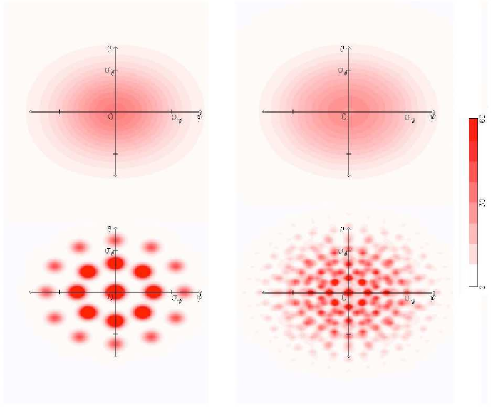
Figure 1: Top: map generated by a single two-dimensional Gaussian centered at the origin, with dispersions $\sigma_{\Phi}=20$ and $\sigma_{\Theta}=15$ (left), and the corresponding maps resulting from applying the high resolution extrapolation method twice (right). Bottom: Artificially refined maps taking a=4 for one (left) and two (right) iterations of the method. Shading is based on a linear scale illustrated at right.

Each time this method is applied it provides 21 new magnetic poles per original one. Therefore, the number of iterations determines the number of new poles and, in consequence, the amount of fine structure being introduced. The top left plot of Figure 1 shows a single Gaussian function with dispersions of $\sigma_{\theta}=15$ and $\sigma_{\phi}=20$ degrees, which are typical values for magnetic poles in these kind of maps. The top right plot of the same figure shows the result of applying the refining algorithm twice to it. This map is generated by a distribution of 441 new Gaussian functions (21 per iteration for each pole). It is clear from the figure that we are able to reproduce very accurately the original Gaussian.

So far we have discussed a method to find one of the possible magnetic maps with fine-structure that in low-resolution would look like the original map. The next step is to find how the high-resolution version of this new map would look. This is straightforward if we keep in mind that, for large enough integration intervals so that the functions die off almost completely inside the integration domain, the following holds

$${\cal{F}}=\int G_{A,\phi_{0},\theta_{0},\sigma_{\phi},\sigma_{\theta}}(\phi,\theta)d\phi\,d\theta\approx$$

$$a^{2}\int G_{A,\phi_{0},\theta_{0},\frac{\sigma_{\phi}}{a},\frac{\sigma_{\theta}}{a}}(\phi,\theta)d\phi\,d\theta$$ (1)

where $\cal{F}$ is the magnetic flux associated with $G_{A,\phi_{0},\theta_{0},\sigma_{\phi},\sigma_{\theta}}(\phi,\theta)$. This property allows us to better resolve the magnetic poles by increasing $a$, while conserving the flux of each one of them by decreasing $\sigma_{\phi,\theta}$ commensurately. Notice that $a$ is a choice that will determine how well resolved the new fine structure given by this method is. In this sense, $a$ is a scale parameter. The bottom panel of Figure 1 shows the result of increasing the parameter $a$ to $4$ for the refined maps after one and two iterations.

3 RESULTS

We simulate the solar wind and the X-ray coronal morphology for the low-resolution solar magnetogram, the same magnetogram with artificially increased spatial resolution, and the high-resolution MDI magnetogram. For the solar wind we perform MHD simulations using the BATS-R-US code and for the X-ray coronal we use the new Low Corona module of the same code.

By applying the HREM to the WSO low-resolution magnetogram we get an artificially increased spatial resolution map (hereafter processed map). The best agreement with the scale of the MDI magnetograms is reached with two iterations and for $a=10$.

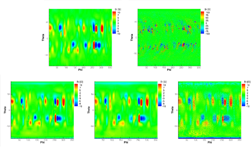
Figure 2: Top: low- and high-resolution observations of the solar magnetic field during Carrington Rotation 1962 (WSO and MDI data). Bottom: Gaussian representation of the WSO low resolution map (left), processed map with $a=1$ (middle), and the processed map with $a=10$ (right).

The top plots of Figure 2 correspond to the WSO and MDI real data magnetograms. While the bottom panel shows the WSO modeled magnetogram (left), the processed map that results from applying two iterations of the HREM to it (middle), and the same map after boosting the scale parameter $a$ from $1$ to $10$ (right). At each iteration the number of poles is increased 21 times, so two iterations result in 441 poles per original one. Nevertheless, the difference in the total flux is only of 1.7 % — excellent agreement considering the large number of new poles that are being introduced. The plots corresponding to the original map and to the high-resolution extrapolation also match qualitatively, as shown in Figure 2 (two bottom left plots). Choosing $a=10$ and applying property (2.2.3) to all the new poles, we are able to better resolve the new magnetogram, thus bringing to light the fine structure lying behind (right bottom plot of Figure 2). This, of course, introduces an error (again, mainly due to the spherical symmetry of the base manifold) which increases with $a$. In our case, where $a=10$, the total flux difference increments to 2.8 %. In consideration of the fairly large uncertainties involved in measuring stellar surface magnetic field strengths we view this is as acceptable taking into account that, since we are dealing with three-dimensional Gaussians, each amplitude is boosted by $a^{2}=100$. Based on the good agreement between the original magnetogram and the new one we construct using this prescription (bottom plots of Figure 2), together with the extremely good conservation of flux, we conclude that the refinement method is robust. It is worth to point out that, as we have already discussed, the new enhanced map is only one of the possible high-resolution maps that would recreate the observed WSO one when smeared, as there is information missing in the WSO map. Therefore we do not expect the processed map to reproduce the MDI map. Our attempt is, rather, to study the effects of introducing fine structure in a reasonable way. By this we mean structure of the same scale of the MDI map and that would recreate the WSO when decreasing its resolution while conserving the original flux, which is different from the MDI flux by two orders of magnitude.

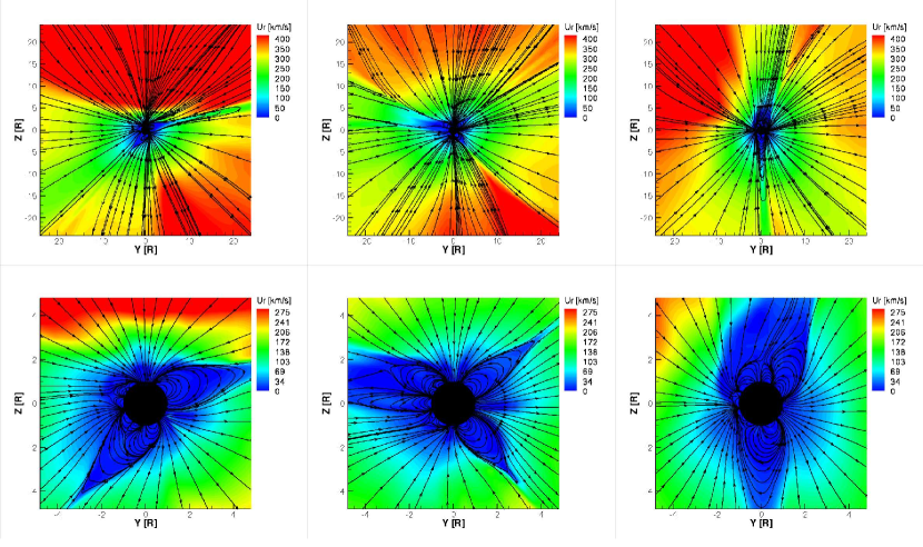
Figure 3: Top: MHD wind solution, displayed on a meridional cut, driven by the low-resolution magnetogram (left), by the processed map (middle), and by the high-resolution MDI magnetogram (right). Bottom: zoomed in images of the same solutions

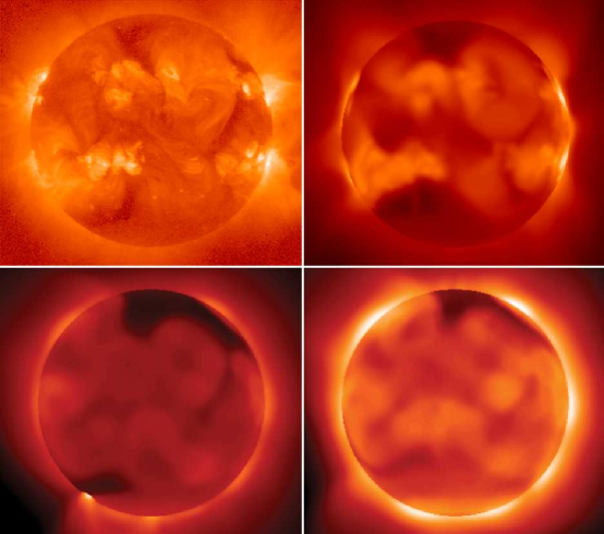
Figure 6: A real X-ray image obtained by Yohkoh contemporaneously with the magnetograms and corresponding to the model viewing angle (top left panel). X-ray emission modeled for the high-resolution MDI map (top right), for the low-resolution magnetogram (bottom left), and for the processed map (bottom right).

The MHD solar wind solutions and the X-ray morphology simulations are shown in Figure 3 and Figure 6 respectively.

3.1 Solar Wind Structure

Using BATS-R-US we simulate the MHD solar wind for three different magnetograms. The WSO low-resolution modeled map (shown in the bottom left plot of Figure 2), the processed map that results from applying twice the HREM algorithm and boosting the parameter $a$ to $10$ (shown in the bottom right plot of Figure 2), and the high-resolution MDI magnetogram (shown in the top right plot of the same Figure). It is worth to point out that, while these magnetograms have different length scales, the runs were performed using the same magnetogram and MHD grid resolution. The wind solutions for these three magnetograms are shown in the top panel of Figure 3 (from left to right respectively).

It is clear that the loop structure changes somewhat when artificially increasing the magnetogram spatial resolution. The streamer near 70 degrees latitude (measured clockwise from the north pole) of the low-resolution driven solution moves slightly towards the north pole, while the one corresponding to a latitude close to 200 degrees moves counterclockwise about 90 degrees. From the zoomed in plots of the same solutions (bottom panel of Figure 3), the shape of the loops near the solar surface can be analyzed in more detail. These show that the latter two streamers also get narrower when artificially increasing the resolution of the magnetogram. One can also see from these close in plots that the small double streamer at latitude 270 degrees becomes much larger, and the double streamer at near 200 degrees becomes a simple streamer for the new solution.

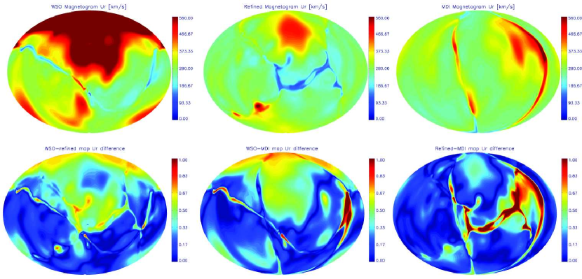
Figure 4: Projection maps of the radial speed for the WSO, the processed map and the MDI driven wind solutions extracted at $r=15R_{sun}$ (top), and the normalized difference between them (bottom).

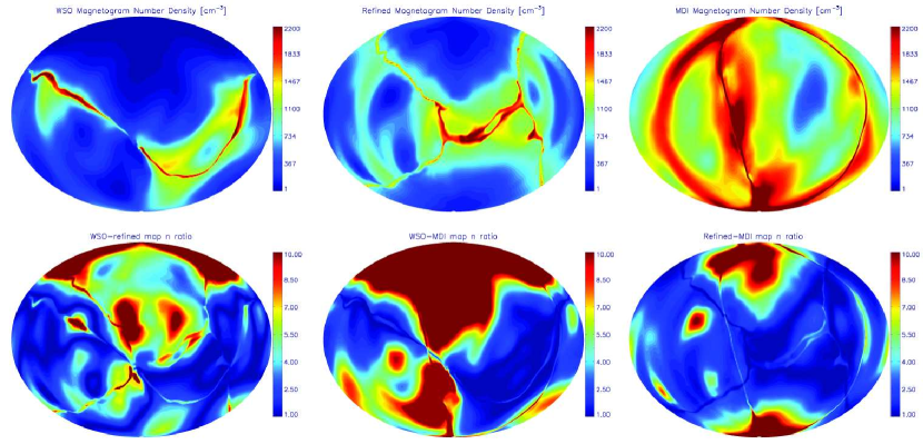
Figure 5: Projection maps of the number density for the WSO, the processed map and the MDI driven wind solutions extracted at $r=15R_{sun}$ (top), and the normalized difference between them (bottom).

For a more quantitative analysis we compare the radial speeds and number densities of the different wind solutions at $15R_{\odot}$. Figure 4 shows the projection maps of the wind radial speeds at $15R_{\odot}$ for the WSO, the processed map and the MDI driven solutions (top panel), and the normalized difference between them (bottom panel). Figure 5 shows the same projection maps for the number densities at the same radial distance. The difference maps are absolute differences normalized to the absolute magnitude of the first one: $abs(u_{1}-u_{2})/abs(u_{1})$. And the ratio is the largest of the ratios between two densities: $max(n_{1}/n_{2},n_{2}/n_{1})$. From the WSO-refined map difference (bottom left plots of both Figures) it is clear that the wind solution changes significantly when introducing fine structure in a consistent way. The wind speed solutions compare better with the MDI solution when the simulations are driven by the processed magnetogram. This is particularly clear from the bottom left plot of Figure 4 when comparing the wind speeds at high latitudes for the low-resolution based solution (left top plot) and the one driven by the processed map (middle top plot), with the MDI driven wind solution (right top plot). In the first case, very fast winds of about 500 km/s reach the $15R_{\odot}$ surface, and even closer to the solar surface (see also top left plot of Figure 3), while this is not the case for the MDI driven solution. This discrepancy is suppressed for the processed magnetic map (top middle plot of Figure 4 and top middle plot of Figure 3).

Interestingly, one can also see that the differences in the refined-MDI plots are much more local than the WSO-MDI. We expect the refined and the MDI driven solutions to be different due to differences in the magnetograms themselves. However, the fact that these differences become more local suggests that the enhanced map performs better when simulating the wind solution.

3.2 X-Ray emission

Corona models for the three magnetograms are compared with the X-ray morphology observed by Yohkoh in Figure 6. Each image is reproduced on a logarithmic scale to provide the dynamic range to see fainter as well as very bright regions. The model driven by the MDI map reproduces very well the bright active regions and some of the loop arcades of the Yohkoh X-ray image. Fine and fainter details are lost, but overall the synthetic image produces a reasonable likeness of the observed one. The low-resolution WSO map solution captures some of the gross active region emission, but fails to separate the active regions near the western limb and loses nearly all the detail, including the active region near the eastern limb at mid-southerly latitude.

A significant amount of structure arises when the resolution of the magnetogram is artificially increased. Many active regions brighten up and start to resolve. In particular, two active regions in the southern hemisphere (one near the center of the equator and the other near the western limb at mid-southerly latitude), two along the equator (one near each limb), and one at high latitudes near the eastern limb, become much more noticeable.

The values of the X-ray fluxes in the images of Figure 6 are: $2\cdot 10^{25}\;ergs\;s^{-1}$ for the WSO solution (bottom left plot), $5\cdot 10^{25}\;ergs\;s^{-1}$ for the processed map solution (bottom right plot), and $1\cdot 10^{27}\;ergs\;s^{-1}$ for the MDI solution (top right plot). The X-ray flux increases $150\%$ when introducing fine-scale structure. Although this increase is rather small as compared to the gap between the WSO and MDI X-ray fluxes, it is clearly in the right direction.

4 DISCUSSION

Our MHD simulations reveal that both the modeled magnetic topology and X-ray morphology are affected by the fine-scale surface magnetic structure.

The wind solution changes significantly when using the MDI solution. The reason for this is that the wind models depend strongly on the expansion factor, defined in Section 2.1. Adding small-scale structure to the magnetogram introduces a new mapping of the magnetic field that changes the distribution of the expansion factors.

When modeling the X-ray emission that originates close to the solar (or stellar) surface, the small-scale magnetic topology of the surface is important. The reason for this is that the field that dominates the closed loop structure and contains the brightest hot, X-ray emitting plasma tends to be relatively small-scaled, and including finer detail can dramatically change the loop structure at low altitude. The high-resolution MDI magnetogram includes areas where there is mixing of polarity. The regions of mixed polarity give rise to the small loops which contribute substantially to the X-ray emission. In the low-resolution version of the magnetogram, these areas are smeared. The mixed polarity regions around the boundaries between larger regions of opposite polarity are lost, and only the large dominant regions of polarity remain. Consequently, the small-scale loop population is lost. In general, then, the low-resolution solution includes a smaller number of larger loops, while in reality the surface is covered by larger number of smaller loops. The large loops obtained by the low-resolution map are not hot and dense enough to compensate for the reduction of simulated X-ray flux from the missing population of smaller low-lying loops. Thus, it is not surprising that the X-ray model solution shows a lot more structure when the magnetogram resolution is artificially increased. There is a slight increase in the X-ray flux for the refined map, but it is rather small. This is probably due to the fact that the refinement does not introduce a significant amount of new closed loops that can contribute to the X-ray flux.

It is observed in solar active regions that areas of one dominant polarity actually comprise bundles of smaller more discrete regions of a dominant polarity with more spatially concentrated magnetic field. The fact that both wind and X-ray morphology solutions show changes when the spatial resolution of the magnetogram is artificially increased suggests that further work is needed to decide whether introducing more mixed polarity (probably hidden within each monopole region) makes a bigger difference. Is the artificially enhanced map more “realistic” than the WSO one? It is tempting to describe the former as better representing the observed Yokoh image than the latter. Lower resolution maps could then be made perhaps slightly more “realistic” by applying the deconvolution and enhancement techniques explored here to include more fine-scale mixed polarity.

A cautionary note has then to be sounded regarding the reconstruction of coronal X-ray emission from stellar ZDI magnetograms. We remarked in Sect. 2.2.1 that stellar magnetograms were generally of a much lower spatial resolution than even the WSO magnetograms. For a star with a complex surface magnetic field distribution, like the active Sun, reconstructed X-ray emission is unlikely to bear a striking resemblance to reality. For the case of very active stars like AB Dor, the situation is less clear. Near the equator, the resolution of AB Dor magnetograms is of a similar order to that of the WSO ones. The key question for the propriety of reconstructed X-ray images regards the true complexity of the surface magnetic field and whether there is a lot of unresolved structure.

Johnstone et al. (2010) and Arzoumanian et al. (2011) note that, since the Zeeman signature is suppressed in the dark spotted regions of the stellar surface, ZDI magnetograms are censored in that they do not reconstruct reliably the field in star spots. Arzoumanian et al. (2011) found that artificially including field with randomly oriented polarity in spotted regions lead to significantly different potential field reconstructions of the coronal morphology and X-ray rotational modulation for AB Dor, but less so for the mostly dipole-dominated M dwarf V374 Peg. Johnstone et al. (2010) also studied the effect of limited spatial resolution using synthetic maps with initial resolution of slightly more than $1\deg$—similar to the WSO maps studied here—and smearing these to latitudinal and longitudinal resolutions of $11\deg$ and $8\deg$ (the latter at the equator). They found that limited spatial resolution does not have a large effect on predicted emission measure for potential field coronal models. Their study covers a much lower resolution regime than we study here though, and the limited sensitivity to spatial resolution is likely partly related to the limited degree of structure at very small spatial scales in their synthetic maps. The existence of compact structures with high plasma densities in active stellar coronae (e.g. Testa et al., 2004; Ness et al., 2002) hints at small-scale magnetic structure. Further investigation of finite resolution effects on the most active stars would be well-motivated.

5 SUMMARY and CONCLUSIONS

Low resolution maps for the magnetic structure of the surface of stars have been widely used to analyze different stellar properties under the assumption that these maps were representative enough for the purposes addressed. This assumption has already been subject to some scrutiny. Using a set of MHD-based simulations of the solar corona and wind, we have investigated how the spatial resolution on scales of $5\deg$ and smaller of the input magnetogram can change the derived structure and morphology of the wind, the magnetic field, and the coronal X-ray emission. We conclude that both wind properties and X-ray morphology are significantly affected by the fine details of the surface magnetic field. The fine-scale structure of the fiducial magnetogram has an impact on the flux tube sizes and expansion factors, therefore affecting the wind solution. Similarly, when modeling the X-ray emission, it becomes crucial to take into account the very small-scale stellar magnetic structure, because it dominates the X-ray emitting loop population. The regions of opposite polarity that support closed loops need to be reasonably well-resolved in order to obtain a realistic X-ray morphology. We find that for both the MHD model wind and the low corona X-ray model, the solution changes significantly when artificially increasing the resolution of the magnetogram by dividing magnetic poles into bundles of stronger but more compact magnetic flux. This fake enhancement also arguably results in perhaps slightly more “realistic” synthetic coronal X-ray images.

References

- Abbett (2007) Abbett, W. P. 2007, ApJ, 665, 1469
- Altschuler & Newkirk (1969) Altschuler, M. D., & Newkirk, G. 1969, Sol. Phys., 9, 131
- Arge & Pizzo (2000) Arge, C. N., & Pizzo, V. J. 2000, J. Geophys. Res., 105, 10,465
- Arzoumanian et al. (2011) Arzoumanian, D., Jardine, M., Donati, J.-F., Morin, J., & Johnstone, C. 2011, MNRAS, 410, 2472
- Aschwanden (2004) Aschwanden, M. J. 2004, Physics of the Solar Corona. An Introduction
- Barnes et al. (1998) Barnes, J. R., Collier Cameron, A., Unruh, Y. C., Donati, J. F., & Hussain, G. A. J. 1998, MNRAS, 299, 904
- Brickhouse & Dupree (1998) Brickhouse, N. S., & Dupree, A. K. 1998, ApJ, 502, 918
- Brickhouse et al. (2001) Brickhouse, N. S., Dupree, A. K., & Young, P. R. 2001, ApJ, 562, L75
- Catala et al. (2007) Catala, C., Donati, J.-F., Shkolnik, E., Bohlender, D., & Alecian, E. 2007, MNRAS, 374, L42
- Cohen et al. (2010a) Cohen, O., Drake, J. J., Kashyap, V. L., Hussain, G. A. J., & Gombosi, T. I. 2010a, ApJ, 721, 80
- Cohen et al. (2010b) Cohen, O., Drake, J. J., Kashyap, V. L., Korhonen, H., Elstner, D., & Gombosi, T. I. 2010b, ApJ, 719, 299
- Cohen et al. (2007) Cohen, O., Sokolov, I. V., Roussev, I. I., Arge, C. N., Manchester, W. B., Gombosi, T. I., Frazin, R. A., Park, H., Butala, M. D., Kamalabadi, F., & Velli, M. 2007, Astrophys. J., 654, L163
- Cohen et al. (2008) Cohen, O., Sokolov, I. V., Roussev, I. I., & Gombosi, T. I. 2008, Journal of Geophysical Research (Space Physics), 113, 3104
- Dempster et al. (1977) Dempster, A. P., Laird, N. M., & Rubin, D. B. 1977, Journal of the Royal Statistical Society. Series B (Methodological), 39, pp. 1
- Donati & Collier Cameron (1997a) Donati, J., & Collier Cameron, A. 1997a, MNRAS, 291, 1
- Donati et al. (1999) Donati, J., Collier Cameron, A., Hussain, G. A. J., & Semel, M. 1999, MNRAS, 302, 437
- Donati & Collier Cameron (1997b) Donati, J.-F., & Collier Cameron, A. 1997b, MNRAS, 291, 1
- Donati et al. (2003) Donati, J.-F., Collier Cameron, A., Semel, M., Hussain, G. A. J., Petit, P., Carter, B. D., Marsden, S. C., Mengel, M., López Ariste, A., Jeffers, S. V., & Rees, D. E. 2003, MNRAS, 345, 1145
- Donati et al. (2008a) Donati, J.-F., Jardine, M. M., Petit, P., Morin, J., Bouvier, J., Collier Cameron, A., Delfosse, X., Dintrans, B., Dobler, W., Dougados, C., Ferreira, J., Forveille, T., Gregory, S. G., Harries, T., Hussain, G. A. J., Menard, F., & Paletou, F. 2008a, in Astronomical Society of the Pacific Conference Series, Vol. 384, 14th Cambridge Workshop on Cool Stars, Stellar Systems, and the Sun, ed. G. van Belle, 156–+
- Donati & Landstreet (2009) Donati, J.-F., & Landstreet, J. D. 2009, ARA&A, 47, 333
- Donati et al. (2010) Donati, J.-F., Morin, J., Petit, P., Delfosse, X., Forveille, T., Auriere, M., Cabanac, R., Dintrans, B., Fares, R., Gastine, T., Jardine, M. M., Lignieres, F., Paletou, F., Ramirez Velez, J. C., & Theado, S. 2010, VizieR Online Data Catalog, 7390, 545
- Donati et al. (2008b) Donati, J.-F., Morin, J., Petit, P., Delfosse, X., Forveille, T., Aurière, M., Cabanac, R., Dintrans, B., Fares, R., Gastine, T., Jardine, M. M., Lignières, F., Paletou, F., Velez, J. C. R., & Théado, S. 2008b, MNRAS, 390, 545
- Downs et al. (2010) Downs, C., Roussev, I. I., van der Holst, B., Lugaz, N., Sokolov, I. V., & Gombosi, T. I. 2010, ApJ, 712, 1219
- Drake et al. (1994) Drake, J. J., Brown, A., Patterer, R. J., Vedder, P. W., Bowyer, S., & Guinan, E. F. 1994, ApJ, 421, L43
- Drake et al. (2000) Drake, J. J., Kashyap, V. L., Audard, M., & Guedel, M. 2000, in Bulletin of the American Astronomical Society, Vol. 32, American Astronomical Society Meeting Abstracts #196, 762–+
- Fares et al. (2010) Fares, R., Donati, J., Moutou, C., Jardine, M. M., Grießmeier, J., Zarka, P., Shkolnik, E. L., Bohlender, D., Catala, C., & Cameron, A. C. 2010, MNRAS, 406, 409
- Favata et al. (2005) Favata, F., Flaccomio, E., Reale, F., Micela, G., Sciortino, S., Shang, H., Stassun, K. G., & Feigelson, E. D. 2005, ApJS, 160, 469
- Favata & Schmitt (1999) Favata, F., & Schmitt, J. H. M. M. 1999, A&A, 350, 900
- Giampapa et al. (1985) Giampapa, M. S., Golub, L., Peres, G., Serio, S., & Vaiana, G. S. 1985, ApJ, 289, 203
- Giampapa et al. (1996) Giampapa, M. S., Rosner, R., Kashyap, V., Fleming, T. A., Schmitt, J. H. M. M., & Bookbinder, J. A. 1996, Astrophys. J., 463, 707
- Gilbert et al. (2007) Gilbert, J. A., Zurbuchen, T. H., & Fisk, L. A. 2007, ApJ, 663, 583
- Groth et al. (2000) Groth, C. P. T., De Zeeuw, D. L., Gombosi, T. I., & Powell, K. G. 2000, J. Geophys. Res., 105, 25053
- Güdel (2007) Güdel, M. 2007, Living Reviews in Solar Physics, 4, 3
- Güdel et al. (2003) Güdel, M., Arzner, K., Audard, M., & Mewe, R. 2003, A&A, 403, 155
- Guedel et al. (1997a) Guedel, M., Guinan, E. F., & Skinner, S. L. 1997a, ApJ, 483, 947
- Guedel et al. (1997b) —. 1997b, ApJ, 483, 947
- Guedel et al. (1995a) Guedel, M., Schmitt, J. H. M. M., & Benz, A. O. 1995a, A&A, 293, L49
- Guedel et al. (1995b) Guedel, M., Schmitt, J. H. M. M., Benz, A. O., & Elias, II, N. M. 1995b, A&A, 301, 201
- Hussain et al. (2005) Hussain, G. A. J., Brickhouse, N. S., Dupree, A. K., Jardine, M. M., van Ballegooijen, A. A., Hoogerwerf, R., Collier Cameron, A., Donati, J.-F., & Favata, F. 2005, ApJ, 621, 999
- Hussain et al. (2007) Hussain, G. A. J., Jardine, M., Donati, J.-F., Brickhouse, N. S., Dunstone, N. J., Wood, K., Dupree, A. K., Collier Cameron, A., & Favata, F. 2007, MNRAS, 377, 1488
- Hussain et al. (2002) Hussain, G. A. J., van Ballegooijen, A. A., Jardine, M., & Collier Cameron, A. 2002, ApJ, 575, 1078
- Jardine et al. (2002a) Jardine, M., Collier Cameron, A., & Donati, J.-F. 2002a, MNRAS, 333, 339
- Jardine et al. (2002b) Jardine, M., Wood, K., Collier Cameron, A., Donati, J.-F., & Mackay, D. H. 2002b, MNRAS, 336, 1364
- Järvinen et al. (2005) Järvinen, S. P., Berdyugina, S. V., & Strassmeier, K. G. 2005, A&A, 440, 735
- Jian et al. (2011) Jian, L. K., Russell, C. T., Luhmann, J. G., MacNeice, P. J., Odstrcil, D., Riley, P., Linker, J. A., Skoug, R. M., & Steinberg, J. T. 2011, Sol. Phys., 273, 179
- Johnstone et al. (2010) Johnstone, C., Jardine, M., & Mackay, D. H. 2010, MNRAS, 404, 101
- Kochukhov et al. (2010) Kochukhov, O., Makaganiuk, V., & Piskunov, N. 2010, A&A, 524, A5+
- Maggio & Peres (1997) Maggio, A., & Peres, G. 1997, A&A, 325, 237
- Manset & Donati (2003) Manset, N., & Donati, J. 2003, in Society of Photo-Optical Instrumentation Engineers (SPIE) Conference Series, Vol. 4843, Society of Photo-Optical Instrumentation Engineers (SPIE) Conference Series, ed. S. Fineschi, 425–436
- Marino et al. (2003) Marino, A., Micela, G., Peres, G., & Sciortino, S. 2003, A&A, 407, L63
- Marsden et al. (2006) Marsden, S. C., Donati, J.-F., Semel, M., Petit, P., & Carter, B. D. 2006, MNRAS, 370, 468
- McGregor et al. (2011) McGregor, S. L., Hughes, W. J., Arge, C. N., Owens, M. J., & Odstrcil, D. 2011, Journal of Geophysical Research (Space Physics), 116, 3101
- McIvor et al. (2003) McIvor, T., Jardine, M., Collier Cameron, A., Wood, K., & Donati, J.-F. 2003, MNRAS, 345, 601
- Mikić et al. (1999) Mikić, Z., Linker, J. A., Schnack, D. D., Lionello, R., & Tarditi, A. 1999, Physics of Plasmas, 6, 2217
- Mok et al. (2008) Mok, Y., Mikić, Z., Lionello, R., & Linker, J. A. 2008, ApJ, 679, L161
- Mullan et al. (2006) Mullan, D. J., Mathioudakis, M., Bloomfield, D. S., & Christian, D. J. 2006, ApJS, 164, 173
- Ness et al. (2002) Ness, J.-U., Schmitt, J. H. M. M., Burwitz, V., Mewe, R., Raassen, A. J. J., van der Meer, R. L. J., Predehl, P., & Brinkman, A. C. 2002, A&A, 394, 911
- Parker (1958) Parker, E. N. 1958, ApJ, 128, 664
- Pneuman & Kopp (1971) Pneuman, G. W., & Kopp, R. A. 1971, Sol. Phys., 18, 258
- Powell et al. (1999) Powell, K. G., Roe, P. L., Linde, T. J., Gombosi, T. I., & de Zeeuw, D. L. 1999, Journal of Computational Physics, 154, 284
- Preibisch (1997) Preibisch, T. 1997, A&A, 320, 525
- Redner & Walker (1984) Redner, R. A., & Walker, H. F. 1984, SIAM Review, 26, 195
- Riley et al. (2012) Riley, P., Linker, J. A., Lionello, R., & Mikic, Z. 2012, Journal of Atmospheric and Solar-Terrestrial Physics, 83, 1
- Riley et al. (2006) Riley, P., Linker, J. A., Mikić, Z., Lionello, R., Ledvina, S. A., & Luhmann, J. G. 2006, ApJ, 653, 1510
- Roussev et al. (2003) Roussev, I. I., Gombosi, T. I., Sokolov, I. V., Velli, M., Manchester, IV, W., DeZeeuw, D. L., Liewer, P., Tóth, G., & Luhmann, J. 2003, ApJ, 595, L57
- Schmitt & Favata (1999) Schmitt, J. H. M. M., & Favata, F. 1999, Nature, 401, 44
- Schmitt & Kurster (1993) Schmitt, J. H. M. M., & Kurster, M. 1993, Science, 262, 215
- Schrijver & Aschwanden (2002) Schrijver, C. J., & Aschwanden, M. J. 2002, ApJ, 566, 1147
- Schrijver et al. (1989) Schrijver, C. J., Lemen, J. R., & Mewe, R. 1989, ApJ, 341, 484
- Schrijver et al. (2004) Schrijver, C. J., Sandman, A. W., Aschwanden, M. J., & De Rosa, M. L. 2004, ApJ, 615, 512
- Sciortino et al. (1999) Sciortino, S., Maggio, A., Favata, F., & Orlando, S. 1999, A&A, 342, 502
- Stern et al. (1986) Stern, R. A., Antiochos, S. K., & Harnden, Jr., F. R. 1986, ApJ, 305, 417
- Strassmeier & Rice (1998) Strassmeier, K. G., & Rice, J. B. 1998, A&A, 330, 685
- Suess & Nerney (1999) Suess, S. T., & Nerney, S. 1999, in ESA Special Publication, Vol. 448, Magnetic Fields and Solar Processes, ed. A. Wilson & et al., 1101–+
- Testa et al. (2004) Testa, P., Drake, J. J., & Peres, G. 2004, ApJ, 617, 508
- Tóth et al. (2005) Tóth, G., Sokolov, I. V., Gombosi, T. I., Chesney, D. R., Clauer, C. R., De Zeeuw, D. L., Hansen, K. C., Kane, K. J., Manchester, W. B., Oehmke, R. C., Powell, K. G., Ridley, A. J., Roussev, I. I., Stout, Q. F., Volberg, O., Wolf, R. A., Sazykin, S., Chan, A., Yu, B., & Kóta, J. 2005, Journal of Geophysical Research (Space Physics), 110, 12226
- Tóth et al. (2011) Tóth, G., van der Holst, B., & Huang, Z. 2011, ApJ, 732, 102
- Usmanov (1993) Usmanov, A. V. 1993, Sol. Phys., 146, 377
- Usmanov & Goldstein (2003) Usmanov, A. V., & Goldstein, M. L. 2003, in American Institute of Physics Conference Series, Vol. 679, Solar Wind Ten, ed. M. Velli, R. Bruno, F. Malara, & B. Bucci, 393–398
- Vaiana & Rosner (1978) Vaiana, G. S., & Rosner, R. 1978, ARA&A, 16, 393
- Ventura et al. (1998) Ventura, R., Maggio, A., & Peres, G. 1998, A&A, 334, 188
- Vogt & Penrod (1983) Vogt, S. S., & Penrod, G. D. 1983, PASP, 95, 565
- Wang & Sheeley (1990) Wang, Y.-M., & Sheeley, N. R. 1990, ApJ, 355, 726
- Wu (1983) Wu, C. F. J. 1983, The Annals of Statistics, 11, pp. 95
- Wu et al. (1999) Wu, S. T., Guo, W. P., Michels, D. J., & Burlaga, L. F. 1999, J. Geophys. Res., 1041, 14789