H-ATLAS: The Cosmic Abundance of Dust from the Far-Infrared Background Power Spectrum

Abstract

We present a measurement of the angular power spectrum of the cosmic far-infrared background (CFIRB) anisotropies in one of the extragalactic fields of the Herschel Astrophysical Terahertz Large Area Survey (H-ATLAS) at 250, 350 and 500 µm bands. Consistent with recent measurements of the CFIRB power spectrum in Herschel-SPIRE maps, we confirm the existence of a clear one-halo term of galaxy clustering on arcminute angular scales with large-scale two-halo term of clustering at 30 arcminutes to angular scales of a few degrees. The power spectrum at the largest angular scales, especially at 250 $\mu$m, is contaminated by the Galactic cirrus. The angular power spectrum is modeled using a conditional luminosity function approach to describe the spatial distribution of unresolved galaxies that make up the bulk of the CFIRB. Integrating over the dusty galaxy population responsible for the background anisotropies, we find that the cosmic abundance of dust, relative to the critical density, to be between $\Omega_{\rm dust}=10^{-6}$ and $8\times 10^{-6}$ in the redshift range $z\sim 0-3$. This dust abundance is consistent with estimates of the dust content in the Universe using quasar reddening and magnification measurements in the SDSS.

1. Introduction

While the total intensity of the cosmic far infrared background (CFIRB) is known from absolute photometry measurements (Puget et al., 1996; Fixen et al., 1998; Dwek et al., 1998), we still lack a complete knowledge of the sources, in the form of dusty star-forming galaxies, that make up the background. Limited by aperture sizes and the resulting source confusion noise (Nguyen et al., 2010), existing deep surveys with the Herschel Space Observatory (Pilbratt et al. 2010) and ground-based sub-mm and mm-wave instruments resolve anywhere between 5 and 15% of the background into individual galaxies (Coppin et al., 2006; Scott et al., 2010; Oliver et al., 2010; Clements et al., 2010; Berta et al., 2011). Anisotropies of the CFIRB, or the spatial fluctuations of the background intensity, provide additional statistical information on the fainter galaxies, especially those that make up the bulk of the background.

While the fainter galaxies are individually undetected, due to gravitational growth and evolution in the large-scale structure these galaxies are expected to be clustered (Cooray2010; Maddox et al., 2010; Hickox et al., 2010; Kampen et al., 2012). In the ansatz of the halo model (Cooray & Sheth, 2002) such clustering of galaxies captures certain properties of the dark matter halos in which galaxies are found and the statistics of how those galaxies occupy the dark matter halos. The resulting anisotropies of the CFIRB are then a reflection of the spatial clustering of galaxies and their infrared luminosity. These CFIRB anisotropies, are best studied from the angular power spectrum of the background infrared light. Separately, statistics such as the probability of deflection, $P(D)$ (Glenn et al., 2010), probe the variance and higher order cumulant statistics of the intensity variations at the beam scale.

While early attempts to measure the angular power spectrum of the CFIRB resulted in low signal-to-noise measurements (Lagache et al., 2007; Viero et al., 2009), a first clear detection of the CFIRB power spectrum with Herschel-SPIRE (Griffin et al. 2010) maps between 30 arcseconds and 30 arcminute angular scales was reported in Amblard et al., (2011). Those first measurements also confirmed the interpretation that galaxies at the peak epoch of star formation in the Universe at redshifts of 1 to 3 trace the underlying dark matter halo distribution. Since then, additional measurements of the CFIRB power spectrum have come from Planck (Planck collaboration, 2011) and with additional SPIRE maps from the HerMES survey (Viero et al., 2012). With multiple fields spanning up to 20 deg², recent HerMES CFIRB power spectra probe angular scales of about 30″  to 2^∘. The halo model interpretation of the HerMES spectra suggest that the halo mass scale for peak star-formation activity is $\log M_{\rm peak}/M_{\sun}\sim 13.9\pm 0.6$ and the minimum halo mass to host dusty galaxies is $\log M_{\rm min}/M_{\sun}\sim 10.8\pm 0.6$.

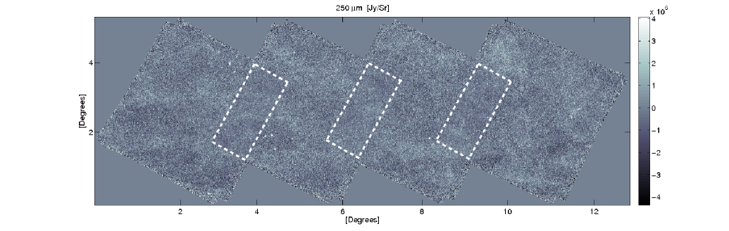
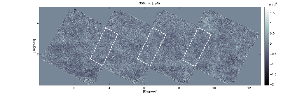
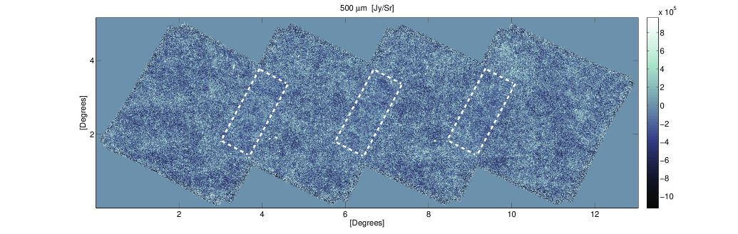
Figure 1.— The Herschel-ATLAS GAMA-15 maps at 250 (top), 350 (middle) and 500 (bottom) $\mu$m with the three overlap regions used for the angular power spectrum measurements highlighted in dashed lines.

The angular power spectrum of CFIRB, in principle, captures the spatial distribution of the background intensity, regardless of whether the emission is from individual point sources or from smoothly varying diffuse sources, such as intracluster and intrahalo dust. Thus the angular power spectrum should be a sensitive probe of the total dust content in the Universe. The existing estimes of the dust abundance from direct emission measurements make use of the sub-mm luminosity (e.g., Dunne, Eales & Edmunds 2003) or dust mass (e.g., Dunne et al. 2011) functions, they are generally based out of extrapolations of the measured bright galaxy counts. The anisotropy power spectrum should capture the integrated emission from faint sources, especially at the flux density scale that dominate the confusion noise. Separately, other estimates of the cosmic dust abundance rely on the extinction of optical light, especially with measurements that combine magnification and extinction of quasars behind samples of foreground galaxies (Menard et al., 2010; 2012). It will be helpful to compare our direct emission measurement of the dust abundance with the extinction-based estimates since any differences can allow us to understand the important of galaxies with hot dust that could be missed in SPIRE maps. We make use of a halo model to interpret the anisotropy power spectrum with the goal of measuring $\Omega_{\rm dust}(z)$, the cosmic abundance of dust relative to the critical density, as a function of redshift.

To enable these measurements we make use of the wide field ($\sim$ 45 deg²) maps of Herschel-ATLAS (Eales et al. 2010) in the three GAMA areas along the equator, and select a single area that has the least Galactic cirrus confusion. This GAMA-15 field involves 4 independent blocks of about 14 deg², each overlapping with the adjacent blocks by about 4 deg². We make use of the three overlap areas between the blocks to measure the power spectra at 250, 350 and 500 $\mu$m. The final power spectrum is the average of the individual power spectra of each of the overlapping regions. While this forces us to make a measurement over a smaller area than the total survey area, our power spectrum measurement has the advantage that with two sets of cross-linked scans we can make independent measurements of the noise power spectrum.

Our measurement approach is similar to that used for HerMES power spectra measurements (Amblard et al. 2011; Viero et al. 2012) using multiple scans to generate jack-knives of data to test the noise model. The total area used in HerMES measurements is about 12 and 60 deg², respectively, in Amblard et al. (2011) and Viero et al. (2012). However, H-ATLAS covers about 120 deg² in all three GAMA fields A measurement of the power spectrum in the whole of H-ATLAS GAMA areas requires an assumption about the noise power spectrum, since in regions with only one orthogonal scan or a single cross-linkeds scan, we are not able to separate the noise from the signal with data alone. In a future paper, we will present the power spectrum of the whole area using a noise model that is independently tested on various datasets to improve the confidence in separating noise in single cross-link scans. For now, we make use of two cross-link scans for cross-correlations and auto-correlations to separate noise and sky signal.

This paper is organized as follows. In Section 2, we briefly review how 250, 350 and 500 $\micron$ maps for the GAMA-15 field were constructed using HIPE (Ott et al., 2010) from raw time streams. In Section 3, we discuss how the auto and cross-correlation functions for each of the three fields were estimated, corrected, and assigned errors. The final power spectra are presented in Section 4. The halo model used to fit the data and the luminosity function is discussed in Section 5. Finally, in Section 6 & 7 we present our results and their implications, discuss future follow up work and give our concluding thoughts.

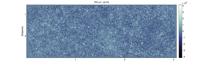
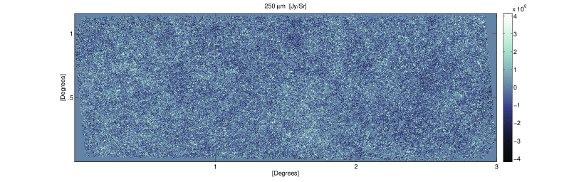
Figure 2.— The left overlap region in Fig. 1 at 250 $\mu$m Herschel-ATLAS showing details of the background intensity variations without (top) and with (bottom) $S>50$ mJy the bright source mask applied. This mask removes a substantial number of low-z bright galaxies detected in the areas used for the fluctuation study.

2. Map Making

For this work we generate SPIRE maps using the MADmap (Cantalupo et al, 2009) algorithm that is available within HIPE. The timeline data were reduced internally by the H-ATLAS team using HIPE version 8.2.0 (Pascale et al., 2011). The timelines were calibrated with corrections applied for the temperature-drift and deglitched both manually and automatically. Astrometry corrections were also applied to the timelines using offsets between SDSS sources and the cross-identifications (Smith et al., 2011). In addition, a scan-by-scan baseline polynomial remover was applied to remove gain variations leading to possible stripes.

The map-maker, MADmap, converts the timeline data $d(t)$

$$d(t)=n(t)+A(p,t)\times s(p)\,,$$ (1)

with noise $n(t)$ and sky signal $s(p)$, given the pointing matrix $A(p,t)$ between pixel and time domain to a map by solving the equation

$$m=(A^{\mathrm{T}}N^{-1}A)^{-1}A^{\mathrm{T}}N^{-1}d\,.$$ (2)

Here $N$ is the time noise covariance matrix and $m$ is the pixel domain maximum likelihood estimate of the noiseless signal map given $N$ and $d$. We refer the reader to Cantalupo et al, (2009) for more details of MADmap.

The final maps we use for this work consist of four partially overlapping tiles, each containing two sets of 96 scans in orthogonal directions (Fig. 1). The pixel-scale for the 250, 350 and 500 $\mu$m maps is 6″, 8.333″  and 12″, respectively, corresponding to $1/3$ of the beam size.

In regions where the tiles do not overlap, the map at each wavelength consists of a single scan each in the two orthogonal scan directions. In the overlap region, we have two scans in each direction. As discussed below, we are able to estimate the noise and signal power spectra independent of each other using the auto-correlations of the combined 4-scan map and the cross-correlations involving various jack-knife combinations. In Fig. 2 we show an example overlap region.

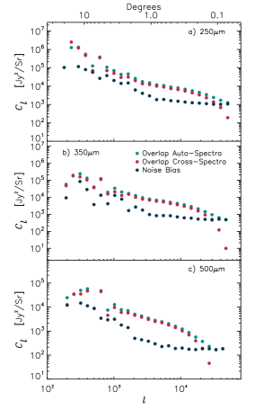
Figure 3.— The raw $C_{l}$ of the GAMA-15 overlap regions at 250 (top), 350 (middle) and 500 (bottom) $\mu$m, respectively. The green points show the auto-power spectra computed from overlap regions using all 4 scans. This power spectrum is a combination of the real sky anisotropy power spectrum and the instrumental noise. We estimate the sky signal independent of noise by creating two sets of maps for each of the three overlap regions with two orthogonal scans each and then taking the cross power spectrum (red points) of those independent maps. The difference of these two spectra shows the instrumental noise power spectrum (black points).

3. Power Spectra

We now discuss the measurement of angular anisotropy power spectra in each of the three SPIRE bands. To be consistent with previous measurements of the SPIRE angular power spectrum (Amblard et al., 2011) our maps are masked by taking a 50 mJy/beam flux cut and then convolving with the point response function. Such a flux cut, through a mask that removes the bright galaxies, also minimizes the bias coming from those bright sources by reducing shot-noise effects. The same mask also includes a small number of pixels that do not contain any useful data, either due to scan strategy or data corruption. The combined mask removes roughly 13, 12 and 15% of the pixels at 250, 350 and 500 $\mu$m, respectively. The fractions of masked pixels are substantially higher than the fractions of Amblard et al. (2011) of 1 to 2% as the ATLAS GAMA-15 field has a large density of $z<0.1$ spiral galaxies over its area relative to more typical extragalactic fields used in the Amblard et al. (2011) study. These galaxies tend to be brighter, especially at 250 $\mu$m. While the fraction masked is larger, the total number of pixels used for this study is comparable to Amblard et al. (2011) with $2.9\times 10^{6}$, $1.5\times 10^{6}$ and $7.0\times 10^{5}$ at 250, 350 and 500 $\micron$ in each of the three overlap regions.

To measure the power spectrum in the final set of maps, we make use of 2D Fourier transforms. In general this is done with masked maps of the overlap regions, denoted $M_{1}$ and $M_{2}$ in real space. If we denote the 2D Fourier transform of each map as $\widetilde{M}_{1}$ and $\widetilde{M}_{2}$, the power spectrum, $C_{l}$, formed for a specific $l$ bin between between $l$-modes $l_{1}$ and $l_{2}$, is the mean of the squared Fourier modes $\tilde{M}_{1}\tilde{M}^{*}_{2}$ between $l_{1}$ and $l_{2}$. The same can be used to describe the auto power spectra, but with $M_{1}=M_{2}$.

The raw power spectra are summarized in Fig. 3. Here, we show the auto spectra in the total map, as well as the cross spectrum with maps made with half of the time-ordered data in each map. The difference of the two provides us with an estimate of the instrumental noise. At small angular scales (large $\ell$ values) the noise follows a white-noise power spectrum, with $C_{l}$ equal to a constant. At large angular scales, the detectors show the expected $1/f$-type of noise behavior, with the noise power spectrum rising as $C_{l}\propto l^{-2}$. We fit a model of the form

$$N_{l}=N_{0}\left[\left(\frac{l_{0}}{l}\right)^{2}+1\right]\,,$$ (3)

and determine the knee-scale of the $1/f$ noise and the amplitude of noise power spectra. The noise values are $N_{0}=1.2\times 10^{3},5.3\times 10^{2}$ and $1.8\times 10^{2}$ Jy²/sr at 250, 350 and 500 $\mu$m, comparable to the detector noise in the 4-scan maps of the Lockman-hole used in Amblard et al. (2011). The knee at which $1/f$ noise becomes important is $l_{0}=3730,2920$ and 3370, comparable to the expected knee at a wavenumber of 0.15 arcmin^-1 given the scan rate and the known properties of the detectors (Griffin et al., 2010).

The raw spectra we have computed directly from the masked maps are contaminated by several different effects that must be corrected for. These issues are: the resolution damping from the instrumental beam, the filtering in the map-making process, and the fictitious correlations introduced by the bright source and corrupt pixel mask. Including these effects, we can write the measured power spectrum as

$$C_{l}^{\prime}=B^{2}(l)T(l)M_{ll^{\prime}}C_{l^{\prime}}\,,$$ (4)

where $C_{l}^{\prime}$ is the observed power spectrum from the masked map, $B(l)$ is the beam function measured in a map, $T(l)$ is the map-making transfer function, and $M_{ll^{\prime}}$ is the mode coupling matrix resulting from the mask. Here, $C_{l^{\prime}}$ is the true sky power spectrum and is determined by inverting the above equation.

We now briefly discuss the ways in which we either determine or correct for the effects just outlined.

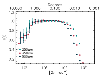
Figure 4.— Map-making transfer function $T(l)$ for the MADmap map making tool used for the GAMA-15 field anisotropy power spectrum measurement. The uncertainties in the transfer function are calculated from 100 random realizations of the sky as described in Section 3.1.

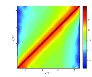
Figure 5.— An example inverse-mode coupling matrix $M_{ll^{\prime}}^{-1}$ for one of the overlap regions (log scale).

3.1. The Map-Making Transfer Function

Due to the finite number of detectors, the scan pattern, and the resulting analysis technique to convert timeline data into a map, the map we produce is not an exact representation of the sky. The modifications are associated with the map-making process, relative to the true sky, are described by the transfer function $T(l)$. We determine this by making 100 random realizations of the sky using Gaussian random fields derived from a first estimate of the H-ATLAS power spectrum. We sample those skies using the same timeline data as the actual observations and analyze the simulated timelines with the same data reduction and map-making HIPE scripts for the actual data. We then compute the average of the ratio between the estimated power spectra and the input spectrum. This function is then the transfer function associated with polynomial filtering and the map-making process. This transfer function, like the beam, represents a multiplicative correction to the data. We divide the estimated power spectrum of the data by this transfer function to remove the map-making pipeline processing effects.

In Fig. 4 we show the transfer functions at 250, 350 and 500 $\mu$m with 68% error bars taken from the standard deviation of 100 simulations. The transfer function is such that it turns over from 1 at both large angular scales, corresponding to roughly the scale of an individual scan length, and the beam scale. The large-scale deviation, which is wavelength independent, is due to the polynomial removal from each timeline of data, while the turnover at small angular scales is due to the cut-off imposed by the instrumental point response function or the beam. The transfer function is more uncertain at the large angular scales due to the finite number of simulations and the associated cosmic variance resulting from the field size. Given its multiplicative nature, errors from this transfer function are added in quadrature with rest of the errors.

3.2. The Beam

Following Amblard et al. (2011), the beam function is derived from Neptune observations of SPIRE. The Neptune timeline data are analyzed with the same pipeline and our default map maker in HIPE. The resulting beam functions are similar to those of Amblard et al. (2011) and we find no detectable changes resulting from the two different map makers between this work and the SMAP (Levenson et al., 2010) pipeline of the SPIRE Instrument Team used in Amblard et al. (2011) and Viero et al. (2012). This is primarily due to the fact that the beam measurements involve a large number of scans and Neptune is several orders of magnitude brighter than the extragalactic confusion noise. We interpolate the beam function measured from Neptune maps in the same $\ell$ modes at which we compute our anisotropy power spectra. This beam transfer function, $B(l)$, at each of the wavelengths represents a multiplicative correction to the data. Similar to Amblard et al. (2011), we compute the uncertainty in the beam function by computing the standard deviation of several different estimates of the beam function by subdividing the scan data to 4 different sets. The error on the beam function in Fourier space is propagated to the final error and is added in quadrature with rest of the errors.

3.3. Mode-Coupling Matrix

The third correction we must make to the raw power spectrum involves the removing of fictitious correlations between modes introduced by the bright sources and contaminated or zero-data pixel mask. Due to this mask the 2D Fourier transforms are measured in maps with holes in them. In the power spectrum these holes result in a Fourier mode coupling that biases the power spectrum lower at large angular scales and higher at smaller angular scales. This can be understood since the modes at the largest angular scales, like the mean of the map, are broken up into smaller scale modes with any non-trivial mask.

To correct for the mask we make use of the method used in Cooray et al., (2012). The method involves capturing the effects of the mask on the power spectrum into a mode-coupling matrix $M_{ll^{\prime}}$. The inverse of the mode coupling matrix then removes the contamination and corrects the raw power spectrum to a power spectrum that should be measurable in an unmasked sky. The correction both restores the power back to the large angular scale modes by shifting the power away from the small angular scale modes, especially those at the modulation scale introduced by the mask.

To generate $M_{ll^{\prime}}$ we apply the mask to a map consisting of a Gaussian realization of a single $l$-mode and take the power spectrum of the resulting map. This power spectrum represents the shuffling of power the mask performs on this specific $l$-mode among the other $l$-modes. This process is repeated for all $l$-modes and these effects of the mask on each mode are then stored in a matrix. This matrix, $M_{ll^{\prime}}$ now represents the transformation from an unmasked to a masked sky by construction. By inverting this matrix, shown in Fig. 5, we are left with the transformation from a masked to an unmasked sky removing the fictitious couplings induced by the mask applied to the raw power spectra. The matrix $M_{ll^{\prime}}$ behaves such that in the limit of no $l-$mode coupling $M_{ll^{\prime}}=f_{\rm sky}\delta_{ll^{\prime}}$ where $f_{\rm sky}$ is the fraction of the sky covered. Thus in the limit of partial sky coverage the correction becomes the standard formula with $C_{l}^{\prime}=f_{\rm sky}C_{l}$. For more details, including figures demonstrating the robustness of the method, we refer the reader to Cooray et al., (2012).

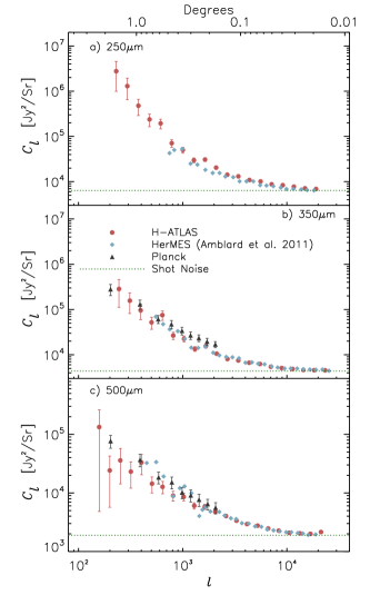
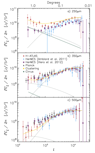
Figure 6.— Final angular power spectra of CFIRB anisotropies in the H-ATLAS GAMA-15 field at 250 (top), 350 (middle) and 500 (bottom) $\mu$m. In the left panels, the power spectra are plotted as $C_{l}$ prior to the removal of the shot-noise term. Here we compare the power spectra measured with H-ATLAS data to Planck and previous Herschel results from HerMES. In the right panels we show the power spectra as $l^{2}C_{l}/2\pi$ after removing the shot-noise level at each of the wave bands. We add the uncertainty associated with the shot-noise level back to the total error budget in quadrature. This results in the increase in errors at high multipoles or small angular scales. The curves show the best-fit model separated into 1 and 2-halo terms (see text for details) and the total (orange line). The solid line that scales roughly as $l^{2}C_{l}\sim l^{-0.9}$ is the best-fit Galactic cirrus fluctuation power spectrum. Due to the high cirrus fluctuation amplitude and clustering, the H-ATLAS power spectrum in the GAMA-15 field at 250 $\mu$m is higher than the existing HerMES results, while the measurements are generally consistent at 350 and 500 $\mu$m.

4. Power Spectrum Results

The final power spectrum $C_{l}$ at each of the three wavelengths is shown in Fig. 6 (left panels). The final error bars account for the uncertainties associated with the (a) beam, (b) map making transfer function, (c) instrumental or detector noise (Fig. 3), and the cosmic variance associated with the finite sky coverage of the field. In Fig. 6 we compare these final H-ATLAS GAMA-15 power spectra with measurements of the CFIRB anisotropy power spectrum measurements from HerMES (Amblard et al. 2011) and Planck (Planck collaboration 2011) team measurements. We find general agreement, but we also find some differences. At 250 $\mu$m, we find the amplitude to be larger than the existing SPIRE measurements of the power spectrum at 250 $\mu$m in HerMES while the measurements are more consistent at 350 and 500 $\mu$m. We attribute this increase to the wide coverage of H-ATLAS and the presence of a large surface density of galaxies at low redshifts. While most of these galaxies are masked we find that the fainter population likely remains unmasked and contributes to the increase in the power that we have seen. This conclusion is also consistent with the strong cross-correlation between detected SPIRE sources in GAMA fields of H-ATLAS and the SDSS redshift survey (e.g., Guo et al. 2011). The difference between Herschel-SPIRE measurements and Planck measurements are discussed in Planck collaboration (2011) and we refer the reader to that discussion. We continue to find differences between our measurements and Planck power spectra at 350 $\mu$m, even with Planck data corrected for the frequency differences and other corrections associated with the source mask, as discussed in Planck collaboration (2011).

Note that the power spectra in the left panels of Fig. 6 asymptote to a $C_{l}\sim$ constant. This is the shot-noise coming from the Poisson behavior of the sources. In Fig. 6 (right panels) we show the final power spectra plotted as $l^{2}C_{l}/2\pi$, with the Poisson noise removed at each band. They now reveal the underlying clustering of submillimeter galaxies. With sources masked down to 50 mJy, our shot-noise amplitudes are $6700\pm 140$, $4400\pm 130$ and $1900\pm 90$ Jy²/sr at 250, 350 and 500 $\mu$m, respectively (see Table 1). We determine the Poisson noise uncertainties based on the overall fit to $C_{l}$ measurements at the three highest $\ell$-bins.

For comparison to our shot-noise values, the shot-noise values of Amblard et al. (2011) are $6100\pm 120$, $4600\pm 70$ and $1800\pm 80$ Jy²/sr at 250, 350 and 500 $\mu$m, respectively. While the shot-noise values are consistent at 350 and 500 $\mu$m, we find an increased shot-noise amplitude at 250 $\mu$m, consistent with the higher amplitude of the clustering part of the power spectrum. In addition to Planck and Amblard et al. (2011) HerMES measurements, in Fig. 6 (right panels) we also compare our measurements to more recent Viero et al. (2012) HerMES measurements. At 350 and 500 $\mu$m the difference between all of Herschel-SPIRE measurements and Planck is clear.

At 250 $\mu$m, we find that our measurements have a higher amplitude at all angular scales relative to previous SPIRE measurements. At large angular scales, we find that the increase is coming from the higher intensity of cirrus in our GAMA-15 fields (Bracco et al. 2011). The cirrus properties as measured from the power spectra are discussed in Section 6.1. As part of the discussion related to our results on the galaxy distribution that is contributing the far-IR background power spectrum (Section 6.2), we will explain the difference between the HerMES and H-ATLAS power spectrum at 250 $\mu$m as due to an excess of low-redshift galaxies in the H-ATLAS GAMA-15 field (Rigby et al. in prep). The measurements shown in Fig. 6 right panels constitute our final CFIRB power spectrum measurements in the H-ATLAS GAMA-15 field. These power spectra values are tabulated in Table 2. We now discuss the model used for the interpretation leading to the best-fit model lines shown in Fig. 6 (right panels).

5. Halo Modeling of the CFIRB Power Spectrum

To analyze the H-ATLAS GAMA-15 power spectra measurements we implement the conditional luminosity function (CLF) approach of Giavalisco & Dickinson, (2001); Lee et al., (2009); De Bernardis & Cooray, (2012). We recall below the main features of the model and refer the reader to these works for more details. The goal is to work out the relation between IR luminosity and halo masses of the galaxies that are contributing to the CFIRB power spectrum. We populate halos with the best-fit $L_{\rm IR}(M)$ relation from the data and use that to determine the abundance of dust ($\Omega_{\rm dust}$) in the Universe. The CLF approach proposed here improves over several assumptions that were made in Amblard et al. (2011) to interpret the first Herschel-SPIRE anisotropy power spectrum measurements.

First, the probability density for a halo or a sub-halo of mass $M$ to host a galaxy with IR luminosity $L$ is modeled as a normal distribution with:

$$P(L|M)=\frac{1}{\sqrt{2\pi}\sigma_{L}(M)}\exp\left[-\frac{(L-\bar{L}(M))^{2}}{2\sigma_{L}(M)^{2}}\right]\,.$$ (5)

The relation between the halo mass and the average luminosity $\bar{L}(M)$ is expected to be an increasing function of the mass with a characteristic mass scale $M_{0l}$ and we can write (see Lee et al., (2009))

$$\bar{L}(M)=L_{0}\left(\frac{M}{M_{0l}}\right)^{\alpha_{l}}\exp\left[-\left(\frac{M}{M_{0l}}\right)^{-\beta_{l}}\right]\,.$$ (6)

As already discussed by Lee et al., (2009) these parameterizations do not have a specific physical motivation, except for the requirement that the luminosity increases as an increasing function of the halo mass and offer the advantage that one can explore a large range of possible shapes for the luminosity-mass relation. While there is no motivation to use this specific form over another, certain models of galaxy formation do predict a $L(M,z)$ relation and our results based out of the model-fits to CFIRB power spectrum can be compared to those model predictions. In particular, the model of Lapi et al. (2011) predicts $L(M,z)\propto M(1+z)^{2.1}$, while the cold-flow accretion model of Dekel et al. (2009) predicts $L(M,z)\propto M^{1.15}(1+z)^{2.25}$.

The total halo mass function is given by the number density of halos or sub-halos of mass $M$. The contribution of halos $n_{h}(M)$ is taken to be the Sheth & Tormen relation (Sheth & Tormen, 1999). The sub-halos term can be modeled through the number of sub-halos of mass $m$ inside a parent halo of mass $M_{p}$, $N(m|M_{p})$. The total mass function is then written as

$$n_{T}(M)=n_{h}(M)+n_{sh}(M)\,,$$ (7)

where $n_{sh}(M)$ is the sub-halo mass function

$$n_{sh}(M)=\int N(M|M_{p})n_{h}(M_{p})dM_{p}\,.$$ (8)

Here we parameterize $N(m|M)$ following the semi-analytical model of van de Bosch et al., (2005).

Neither the normalization nor the slope of the sub-halo mass function are universal and both depend on the ratio between the parent halo mass and the non-linear mass scale, $M_{*}$. $M_{*}$ is defined as the mass scale where the rms of the density field $\sigma(M,z)$ is equal to the critical over-density required for spherical collapse $\delta_{c}(z)$. The contribution of central galaxies to the halo occupation distribution (HOD) is simply the integral of $P(L|M)$ over all luminosities above a certain threshold $L_{0}$, either fixed by the survey or a priori selected so that

$$\langle N_{c}(M)\rangle_{L\geq L_{min}}=\int_{L_{min}}P(L|M)dL\,,$$ (9)

which, in the absence of scatter, reduces to a step function $\Theta(M-M_{0})$, as expected. Note that all integrals over the luminosity $L$ also have a redshift-dependent cut-off at the upper limit corresponding to the flux cut of 50 mJy that we used for the power spectrum measurement. For the satellite galaxies, the HOD is related to the sub-halos

$$\langle N_{s}(M)\rangle_{L\geq L_{min}}=\int_{L_{min}}dL\int dmN(m|M)P(L|m)\,.$$

The total HOD is then

$$\langle N_{\rm tot}(M)\rangle_{L\geq L_{min}}=\langle N_{h}(M)\rangle_{L\geq L_{min}}+\langle N_{sh}(M)\rangle_{L\geq L_{min}}\,.$$

Table 1Parameter values from MCMC fits to the H-ATLAS GAMA-15 angular power spectra at $250$, $350$ and $500$ $\mu$m.

HOD	$\alpha_{l}$	$0.69\pm 0.04$
	$\beta_{l}$	$0.09\pm 0.05$
	$\log(L_{0}/L_{\odot})$	$9.52\pm 0.08$
	$\log(M_{0}/M_{\odot})$	$11.5\pm 1.7$
	$P_{M}$	$-2.9\pm 0.4$
CFIRB SED	$T_{\rm dust}$	$37\pm 2$ K
	$\beta_{\rm dust}$	unconstrained
Cirrus	$C_{250}^{l=230}$	$3.5\pm 1.3\times 10^{5}$ Jy2/sr
	$C_{350}^{l=230}$	$1.2\pm 1.0\times 10^{4}$ Jy2/sr
	$C_{500}^{l=230}$	$1.1\pm 0.9\times 10^{3}$ Jy2/sr
	$T_{\rm cirrus}$	$21.1\pm 1.9$ K
	$\beta_{\rm cirrus}$	$2.9\pm 0.8$
Poisson	$SN_{\rm 250}$	$6700\pm 140$ Jy2/sr
	$SN_{\rm 350}$	$4400\pm 130$ Jy2/sr
	$SN_{\rm 500}$	$1900\pm 90$ Jy2/sr

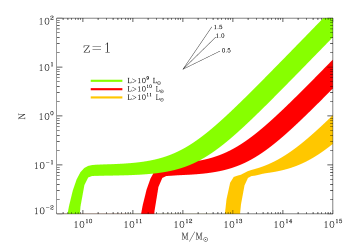
Figure 7.— Best-fit halo occupation distribution and the $1\sigma$ range at $z=1$ for three cases involving $L_{\rm IR}>10^{9},10^{10}$ and 10¹¹ L_☉. The three lines to the top show the different power-laws for comparison with the shape of the HOD. The satellite galaxies contribution has a slope $\sim 1$ when $L_{\rm IR}\sim 10^{9}$ L_☉.

Figure 8.— Luminosity functions predicted by our model compared to data from Eales et al., (2010) $(0.2<z<0.4)$ and Lapi et al., (2011) $(1.2<z<1.6,2<z<2.4)$. The shaded region corresponds to the 68% confidence level.

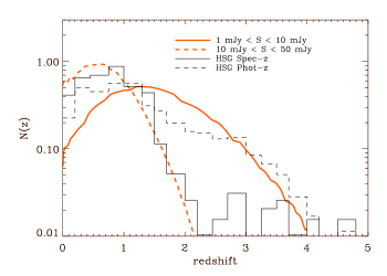
Figure 9.— Normalized redshift distributions of FIR-bright galaxies predicted by our model for two different flux density cuts at 250 $\mu$ (thick solid line for $1\,{\rm mJy}<S<10\,{\rm mJy}$ and thick dashed line for $10\,{\rm mJy}<S<50\,{\rm mJy}$). For comparison in corresponding thin lines we show the measured redshift distributions for the Herschel-selected galaxies (HSGs) at the same flux density bins with optical spectra in Casey et al., (2012).

We account for the possible redshift evolution of the luminosity-halo mass relation by introducing the parameter $p_{M}$ and rewriting the mass scale $M_{0l}$ as:

$$M_{0l}(z)=M_{0l,z=0}(1+z)^{p_{M}}\,.$$ (12)

Under the assumption that the central galaxy is at the center of the halo and that the halo radial profile of satellite galaxies within dark matter halos follow that of the dark matter, given by the Navarro, Frenk and White (NFW) profile (Navarro et al., 1997), we can write the 1-halo and 2-halo terms of the three-dimensional power spectrum:

$$P^{1h}(k)=\frac{1}{n_{g}^{2}}\int dM\langle N_{T}(N_{T}-1)\rangle u(k,M)^{p}n_{h}(M)\,,$$ (13)

where $u(k,M)$ is the NFW profile in Fourier space and $n_{g}$ is the galaxy number density

$$n_{g}=\int dM\langle N_{g}(M)\rangle n_{h}(M)\,.$$ (14)

The second moment of the HOD that appear in eq. 13 can be simplified as

$$\langle N_{T}(N_{T}-1)\rangle\simeq\langle N_{T}\rangle^{2}-\langle N_{h}\rangle^{2}\,,$$ (15)

and the power index $p$ for the NFW profile is $p=1$ when $\langle N_{T}(N_{T}-1)\rangle<1$ and $p=2$ otherwise (Lee et al., 2009).

The two-halo term of galaxy power spectrum is

$$P^{2h}(k) = \left[\frac{1}{n_{g}}\int dM\langle N_{T}(M)\rangle u(k,M)n_{h}(M)b(M)\right]^{2}$$ (16)

$$\times P_{\rm lin}(k)\,,$$

where $P_{\rm lin}(k)$ is the linear power spectrum and $b(M)$ is the linear bias factor calculated as in (Cooray & Sheth, 2002). The total galaxy power spectrum is then $P_{g}(k)=P^{1h}(k)+P^{2h}(k)$.

The observed angular power spectrum can be related to the three-dimensional galaxy power spectrum through a redshift integration along the line of sight (Knox et al., 2001; Amblard & Cooray, 2007):

$$C_{\ell}^{\nu\nu^{\prime}}=\int dz\left(\frac{d\chi}{dz}\right)\left(\frac{a}{\chi}\right)^{2}\bar{j}_{\nu}(z)\bar{j}_{\nu^{\prime}}(z)P_{g}(\ell/\chi,z)\,,$$ (17)

where $\chi$ is the comoving radial distance, $a$ is the scale factor and $\bar{j}_{\nu}(z)$ is the mean emissivity at the frequency $\nu$ and redshift $z$ per comoving unit volume that can be obtained as:

$$\bar{j}_{\nu}(z)=\int dL\phi(L,z)\frac{L}{4\pi}\,.$$ (18)

Here the luminosity function is

$$\phi(L,z)dL=dL\int dMP(L|M)n_{T}(M,z)\,.$$ (19)

To fit data at different frequencies we assume that the luminosity-mass relation in the IR follows the spectral energy distribution (SED) of a modified black-body (here we normalize at $250\mu m$ at $z=0$) with

$$L_{\nu}(M)=L_{250}(M)(1-e^{-\tau})B(\nu_{0},T_{d})\,,$$ (20)

where $T_{d}$ is the dust temperature and the optical depth is $\tau=\left(\frac{\nu_{0}}{\nu}\right)^{\beta_{d}}$ when $B(\nu_{0},T_{d})$ is the Planck function and $L_{250}(M)$ is given by eq (6).

The final power spectrum is a combination of galaxy clustering, shot-noise and the Galactic cirrus such that $C_{l}^{\rm tot}=C_{l}^{\rm CFIRB}+C_{l}^{\rm cirrus}+C_{l}^{\rm SN}$, where $C_{l}^{\rm CFIRB}$ is the power spectrum derived above and $C_{l}^{\rm SN}$ is the scale-independent shot-noise. To account for the Galactic cirrus contribution to the CFIRB, we add to the predicted angular power spectrum a cirrus power-law power spectrum with the same shape of that used by Amblard et al., (2011), where the authors assumed the same cirrus power-law power-spectrum shape from measurements of IRAS and MIPS (Lagache et al., 2007) at $100$ $\mu$m with $C_{l}\propto l^{-n}$ with $n=2.89\pm 0.22$. In Amblard et al. (2011) this 100 $\mu$m spectrum was extended to longer wavelengths using the spectral dependence of Schlegel, (1998). Here we rescale the amplitude of the cirrus power spectrum with amplitudes $C^{\rm cirrus}_{i}$ at each of the three wavelengths ($i=250,350$ and 500 $\mu$) taken to be free parameters and model-fit those three parameters describing the amplitude as part of the global halo model fits with the MCMC approach.

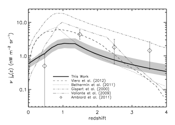
Figure 10.— Best-fit determination of mean emissivity at 250 $\mu$m as a function of the redshift, $\nu j_{\nu}(z)$ (thick solid line), and its 1$\sigma$ error from the MCMC model fits (grey shaded region) for sources with $S_{250}<50$mJy. We show several model predictions from the literature (Valiante et al., 2009; Bethermin et al., 2011) and compare our estimates to the determinations from the halo model fits to the CFIRB power spectra by Amblard et al., (2011) and Viero et al., (2012). Amblard et al., (2011) measurements involve a binned description of $j_{\nu}(z)$ with 1$\sigma$ errors determined from the fit, while Viero et al., (2012) result is the best-fit relation for their work.

6. Results and Discussion

We fit the halo-model described above to the $250$, $350$ and $500$ $\mu$m CFIRB angular power spectrum data for the H-ATLAS GAMA-15 field by varying the halo model parameters and the SED parameters. The dimension of the parameter space is thus $12$ with free parameters involving $T_{d}$, $\beta_{d}$, $\alpha_{l}$, $\beta_{l}$, $L_{0}$, $p_{M}$, $C^{\rm cirrus,l=230}_{i}$ and $SN_{i}$. We make use of a Markov Chain Monte Carlo (MCMC) procedure, modified from the publicly available CosmoMC (Lewis & Bridle, 2002), with a convergence diagnostics based on the Gelman-Rubin criterion (Gelman & Rubin, 1992). To keep the number of free parameters in the halo model manageable, we a priori constrain the $M_{0l}$ in equation 12 to the value of $\log M_{0l}/M_{\sun}=11.5\pm 1.7$ as determined by a fit to the low-redshift luminosity function at 250 $\mu$m (De Bernardis & Cooray, 2012) using data from Vaccari et al. (2010) and Dye et al. (2010). The best fit parameters and the uncertainties from the halo model fits are listed in Table 1.

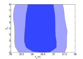
Figure 11.— 68% and 95% confidence level constraints on $T_{d}$ and $\beta_{\mathrm{dust}}$.

6.1. Cirrus Amplitude and Cirrus Dust Temperature

We now discuss some of the results starting from our constraints on the cirrus fluctuations. The cirrus amplitudes have values of $(3.5\pm 1.3)\times 10^{5},(1.2\pm 1.0)\times 10^{4}$ and $(1.1\pm 0.9)\times 10^{3}$ Jy²/sr at 250, 350 and 500 $\mu$m, respectively, at $\ell=230$ corresponding to 100 arcminute angular scales. These values are comparable to the cirrus amplitudes in the Lockman-Hole determined by Amblard et al. (2011). The GAMA-15 area we have used for this study is thus comparabale to some of the least Galactic cirrus contaminated fields on the sky. For comparison, the GAMA 9 hour area studied by Bracco et al. (2011) has cirrus amplitudes of $\sim 3\times 10^{7},2\times 10^{6}$ and $1\times 10^{5}$ at 250, 350 and 500 $\mu$, respectively. These are roughly a factor of 100 larger than the cirrus fluctuation amplitude in the GAMA-15 areas used here. The third field we considered for this study in GAMA 12 hour area was found to have cirrus amplitudes that are roughly a factor of 20 to 30 larger.

In order to determine if the cirrus dust in the GAMA-15 field is comparable to dust in the high cirrus intensity regions such as the GAMA-9 field, we fitted a modified blackbody model to the cirrus rms fluctuation amplitude. We found the dust temperature and the dust emissivity parameter $\beta$ to be $21.1\pm 1.9$ K and $2.9\pm 0.8$, respectively. The results from the same analysis at 100 arcminute-scale rms fluctuations are $20.1\pm 0.9$ and $1.3\pm 0.2$ for dust temperature and emissivity, respectively. Even though the cirrus amplitude is lower with rms fluctuations, $\sqrt{C_{i}^{\rm cirrus}}$, at a factor of 10 below the GAMA-9 area studied in Bracco et al. (2011), we find the dust temperature to be comparable. It is unclear if the difference in the dust emissivity parameter is significant or captures any physical variations in the dust from high to low cirrus intensity, especially given the well-known degeneracy between dust temperature and $\beta$. Fluctuation measurements in all of the 600 sq. degree H-ATLAS fields should allow a measurement of $\beta$ as a function of cirrus amplitude.

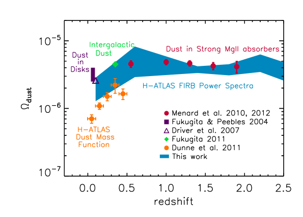
Figure 12.— The cosmic density of dust $\Omega_{dust}$ vs redshift as determined from the CFIRB power spectra from H-ATLAS GAMA-15 field (shaded region). The thickness of the region corresponds to the $1-\sigma$ ranges of the halo model parameter uncertainties as determined by MCMC fits to the data (Table 1). We also compare our estimate to previous measurements in the literature. The measurements labeled H-ATLAS dust mass function are from the low-redshift dust mass function measurements in Dunne et al. (2011). The other estimates are based on extinction measurements from the SDSS (e.g., Ménard et al. 2010, 2012; Fukugita 2011; Fukugita & Peebles 2004) and 2dF (e.g., Driver et al. 2007).

6.2. Faint Star-Forming Galaxy Statistics

Moving to the galaxy distribution, in Fig. 7, we show the halo occupation distribution at $z=1$ corresponding to the best-fit values of the parameters and the $1\sigma$ uncertainty region for three different luminosity cut-off values. At $z=1$, as show in Fig. 7, for $L_{\rm IR}>10^{9}$ L_☉ galaxies, the HOD drops quickly for masses smaller than $\log(M_{\rm min}/M_{\odot})\simeq 10.7$ and the high-mass end has a power-law behavior with a slope $\sim 1$. By design, this halo model based on CLFs has the advantage that it does not lead to unphysical situations with power-law slopes for the HOD greater than one as found by Amblard et al. (2011).

Both the HOD and the underlying luminosity-mass relations are consistent with De Bernardis & Cooray, (2012), where a similar model was used to reinterpret Amblard et al. (2011) anisotropy measurement. The key difference between the work of De Bernardis & Cooray, (2012) and the work here is that we introduce a dust SED to model-fit power spectra measurements in the three wavebands of SPIRE, while in earlier work only 250 $\mu$m measurements were used for the model fit. For comparison with recent model descriptions of the CFIRB power spectrum, we also calculate the effective halo mass scale given by

$$M_{\rm eff}=\int dMn_{h}(M)M\frac{N_{T}(M)}{n_{g}}\,.$$ (21)

With this definition we find $M_{\rm eff}=3.2\times 10^{12}$ M_sun at $z=2$, consistent with the effective mass scales of Shang et al., (2011) and De Bernardis & Cooray, (2012) of $M_{\rm eff}\sim 4\times 10^{12}$ and slightly lower than the value of $\sim 5\times 10^{12}$ from Xia et al., (2012).

The MCMC fits to the CFIRB power spectrum data show that the charicteristic mass scale $M_{0l}$ evolves with redshift as $(1+z)^{-2.9\pm 0.4}$. In order to compare this with existing models, we convert this evolution in the charachteristic mass scale to an evolution of the $L(M,z)$ relation. As $L(M)\propto(M/M_{0l})^{-\alpha_{l}}$, we find $L(M,z)\propto M^{\alpha}_{l}(1+z)^{-p_{M}\alpha_{l}}$. Using the best-fit values, we find $L(M,z)\propto M^{0.70\pm 0.05}(1+z)^{2.0\pm 0.4}$. In Lapi et al. (2011), their equation 9 with the SFR as a measure of the IR luminosity, this relation is expected to be $M(1+z)^{2.1}$. In Dekel et al. (2009), the expectation is $M^{1.15}(1+z)^{2.25}$. While we find a lower value for the power-law dependence on the halo mass with IR luminosity, the redshift evolution is consistent with both these models.

To test the overall consistency of our model relative to existing observations at the bright-end, in Fig. 8, we compare the predicted luminosity functions 250 $\mu$m-selected galaxies in several redshift bins with existing measurements in the literature from Eales et al. (2010) and Lapi et al. (2011). The former relies on the spectroscopic redshifts in GOODS fields while the latter makes use of photometric redshifts. We find the overall agreement to be adequate given the uncertainties in the angular power spectrum and the resulting parameter uncertainties of the halo model. In future, the overall modeling could be improved with a joint-fit to both the angular power spectra and the measured luminosity functions.

In Fig. 9 we show the predicted redshift distributions of the 250 $\mu$m-selected galaxies in two 250-$\mu$m flux density bins in our model with a comparison to a measured redshift distribution with close to 900 optical spectra of Herschel-selected galaxies with Keck/LRIS and DEIMOS in Casey et al. (2012). While there is an overall agreement, for the brighter flux density bin, the measured redshift distribution shows a distinct tail a small, but non-negligible, fraction of galaxies at $z>2$. It is unclear if those redshifts suggest the presence of bright galaxies that are lacking in our halo model or if those redshifts are associated with lensed sub-mm galaxies (Negrello et al., 2010; Wardlow et al., 2012) with intrinstic fluxes that are below 10 mJy. If lensed, due to magnification boost, such fainter galaxies will appear in the brighter bin. We also note that the current halo model ignores any lensing effect in the anisotropy power spectrum. Existing models suggest that the lensing rate at 250 $\mu$m with flux densities below 50 mJy is small. At 500 $\mu$m, however, the lensed counts are at the level of 10% (Wardlow et al. 2012). While we do not have the signal-to-noise ratio for a lensing analysis of the far-IR background anisotropies with the current data and the power spectrum, a future goal of sub-mm anisotropy studies must involve characterizing the lensing modification to the power spectrum.

In Fig. 10 we show the redshift evolution of the emissivity predicted by our model at 250 $\mu$m according to equation 18. The shaded region shows the $1\sigma$ uncertainty associated with the best-fit model. For comparison we show the results of Viero et al., (2012); Valiante et al., (2009); Bethermin et al., (2011); Amblard et al., (2011); Gispert et al., (2000). The distribution predicted by our fit is consistent for a wide range of redshifts (up to $z>3$) with Viero et al., (2012); Valiante et al., (2009); Bethermin et al., (2011); Amblard et al., (2011). The recent fit of Viero et al., (2012) to the HerMES angular power spectra shows a lower emissivity at both low-redshift ($z<0.5$) and high-redshift ($z>2.5$) ends.

The excess in the emissivity at the low-redshifts ($z<0.1$) partly explains the difference in the power spectrum amplitude at 250 $\mu$m between the previous angular power spectra and H-ATLAS data. As discussed earlier, the GAMA-15 field of H-ATLAS is known to contain an overdensity of low-redshift galaxies. The brightest of these sources with $S_{250}>50$ mJy are clearly visible in Fig. 2 when comparing the original and masked maps. While the $S_{250}>50$ mJy mask is expected to remove a substantial fraction of the low-z population, we expect a fraction of the fainter ones to remain. Such galaxies are not present in the well-known extragalactic fields of the HerMES survey such as Lockman-Hole and the NDWFS-Bootes field. The difference is a factor of $\sim$ 2 amplitude increase in the power spectrum at 250 $\mu$m. As the excess population is primarily at low redshifts, the difference only shows up at 250 $\mu$m, while we do not see any significant difference at 350 and 500 $\mu$m between HerMES and H-ATLAS power spectra. The final result of this is to increase the emissivity at 250 $\mu$m at lowest redshifts $z<0.1$ in our model relative to the emissivity function derived in Viero et al., (2012).

The H-ATLAS GAMA-15 field also shows an overall increase of bright counts at 250 $\mu$m relative to the HerMES fields (Rigby et al. in prep) and we verified that our suggestion of a factor of 2 increase in the power spectrum is coming from low-redshift galaxies is consistent with the differences in the number counts. The difference in the counts also explains the increase in the shot-noise at 250 $\mu$m relative to the value found in HerMES power spectra. These differences generally suggest that large field-to-field variations in the angular power spectrum with variations well above the typical Gaussian cosmic variance calculations. Such variations are readily visible when comparing individual field power spectra in Viero et al., (2012) (their Fig. 3).

Through our joint model-fit to 250, 350 and 500 $\mu$m power spectra, we also determine the SED of far-IR background anisotropies. To keep the number of free parameters in our model small, here we assume that the SED can be described by an isothermal black-body model. The best-fit dust temperature value that describes the far-IR fluctuations is $37\pm 2$ K while the emissivity parameter $\beta$ is unconstrained. In Fig. 11 we show the best-fit 68% and 95% confidence level intrvals of $T_{d}$ and $\beta$, after marginalizing over all other parameters of the halo model. This figure makes it clear why we are not able to determine $\beta$ with the current data due to degeneracies between the model parameters. The dust temperature we measure should be considered as the average dust temperature of all galaxies that is contributing to far-IR background anisotropy power spectrum. The dust temperature is higher than the typical 20K dust temperature derived from the absolute background spectra at far-IR wavelengths from experiments such as FIRAS and Planck (Lagache et al., 2000).

This difference in the dust temperature could be understood since the absolute measurements, especially at degree angular-scale beams, are likely to be dominated by the Galactic cirrus, and thus the temperature measurement could be biased low. The dust temperature we measure from the far-IR power spectra is fully consistent with the the value of $44\pm 7$K by Shang et al. (2011) in their modeling of the Planck far-IR power spectra (assuming the fixed value $\beta=2$). Thus, while the best-fit SED model of the absolute CIB may suggest a low temperature value, the anisotropies from approximately 1-30 arcminute angular scales follow a SED with a higher dust temperature value. Separately, we also note that our dust temperature of 37 $\pm 2$ K is also consistent with the average dust temperature values of $36\pm 7$ K (Chapman et al., 2005; Dunne et al., 2000) for high-z SCUBA-selected sub-mm galaxies, but is somewhat higher than the average dust temperature value of $28\pm 8$ K for Herschel-selected bright galaxies in Amblard et al., (2010). The Amblard et al. (2010) value is dominated by low-redshift ($z\sim 0.1$) galaxies with Herschel identifications to SDSS redshifts. In the local Universe, most dusty late-type galaxies show cold dust with temperatures around 20 K (Galametz et al., 2012; Davies et al., 2012). The higher temperature we find for the far-IR background anisotropies then suggests that the average interstellar radiation field in galaxies at $z\sim 1$ to 2 that dominate the dust emissivity is higher by a factor of $2^{6}$ when compared that local late-type galaxies.

6.3. Cosmic Dust Abundance

The model described above allows us to estimate the fractional cosmic dust density:

$$\Omega_{\rm dust}(z)=\frac{1}{\rho_{0}}\int_{L_{min}}dL\phi(L,z)M_{dust}(L)\,,$$ (22)

where $M_{dust}$ is the dust mass for a given IR luminosity and $\rho_{0}$ is the critical density of the Universe. Here we make use $\phi(L,z)$ as derived by the halo model fits to the far-IR background power spectra.

To convert luminosities to dust mass, we follow equation 4 in (Fu et al., 2012). This requires an assumption related to the dust mass absorption coefficient, $\kappa_{d}$. It is generally assumed that the opacity follows $\kappa_{d}(\nu)\propto\nu^{\beta}$ with a normalization of $\kappa_{d}=0.07\pm 0.02$ m² kg^-1 at 850 $\mu$m (Dunne et al., 2000; James et al., 2002). This normalization, unfortunately, is highly uncertain and could easily vary by a factor of few or more (see discussion in James et al. 2002). The value we adopt here is appropriate for dusty galaxies and matches well with the integrated spectrum of the Milky Way.

The conversion to dust mass also requires the SED of dust emission. Here we make use of the average dust temperature value of $37\pm 2$ K as determined by the model-fits to the angular power spectra. As $\beta$ is undetermined from the data, we take its range with a prior between 1 and 2.5, consistent with typical values of 1.5 or 2 that is generally assumed in the literature. When calculating $\Omega_{\rm dust}(z)$ we marginalize over all parameter uncertainties so that we fully capture the full likelihood from the MCMC chains given the prior on $\beta$. Note that our assumption of a constant dust temperature is at odds with local late-type spirals that show much lower temperatures. However, it is also known that there are some sub-mm galaxies, especially those that are radio bright, with dust temperatures in the excess of 60 K. Thus with a value of 37 $\pm 2$ K we may be using a representative average value for the dust temperature and an average of the dust SED for all galaxies at a variety of redshifts. Finally there are some indications that the dust temperature is IR luminosity dependent (see the discussion in Amblard et al. 2010). If that remains to be the case then the correct approch with eq. 22 will be to take into account that luminosity dependence as seen in the observations. Given that the current indications are coming from small galaxy samples, we do not pursue such a correction, but highlight that future studies could improve our dust abundance estimate.

In Fig. 12 we show our results. In addition to the direct emission estimate that we have considered here, we also show the low-z dust abundances by integrating over the dust mass functions in Dunne et al. (2011). Those dust mass functions are limited to $z<0.5$ due to the limited availability of spectroscopic data at higher redshifts. While in principle dust mass function captures the total dust of detected galaxies, the mass functions can be extrapolated to the faint-end, as has been done here, to acocunt for the fainter populations below individual detection levels. Thus the abundances from mass functions must agree with the estimates based on the anisiotropy measurements. We do not use our halo model to estimate the dust abundance at $z<0.05$ since our halo model is normalized to the luminosity function of dusty galaxies at low redshifts.

Our measurement indicates that the dust density ranges between $\Omega_{\rm dust}\simeq 10^{-6}$ to $8\times 10^{-6}$ in the redshift range $z=0.5-3$. We note that the $\Omega_{\rm dust}$ prediction of this work has a smaller uncertainty than that in De Bernardis & Cooray, (2012) where the estimation was done assuming a larger range for $T_{d}$ and $\beta_{d}$. In equation 22 we integrate over luminosities $L>10^{9}$ L_☉. However in this calculation the choice of minimum luminosity is less relevant, since the uncertainty on the dust density estimate is dominated by the large uncertainties of dust temperature and spectral emissivity index $\beta$.

Fig. 12 also summarizes the dust-density measurements of Fukugita & Peebles, (2004); Driver et al., (2007); Menard et al., (2010); Fukugita et al., (2011). We have combined the points from Menard et al. (2010) for the dust contributions of halos and those from Menard & Fukugita, (2012) to a single set of data points, under the assumption that the amount of dust in halos doesn’t evolve significantly with redshift. This is an assumption and could be tested in future data. At high redshifts our estimate is consistent with the results of Fukugita & Peebles, (2004); Driver et al., (2007); Menard et al., (2010).

We note that the Ménard et al. (2010, 2012) measurements assume a reddening law appropriate for the SMC. A Milky Way reddening law would have resulted in a a factor of 1.8 higher dust masses, and thus dust abundance, than the values shown in Fig. 12 (see discussion in Ménard et al. 2012). Since the extinction measurements make use of a reddening law consistent with SMC while the direct emission measurements of the dust abundance that we show here assumed a dust mass absorption coefficient that is more consistent with the Milky Way, it is interesting to ask why the two measurements shown in Fig. 12 agree. The UV reddening law related to extinction based dust abundance estimates comes from small grains that dominate the absorption and scattering surface area. SMC differs from other galaxies in that it does not show a prominent 2200$\AA$ feature, which is assumed to come from carbon bonds. On the other hand, the far-IR emission that we have detected is likely dominated by large grains, usually assumed to be a mixture of silicates and carbonaceous grains. The difference in the reddening law between SMC and Milky Way then should not complicate the abundance estimates since extinction and emission may be coming from different populations of dust grains (e.g., Li & Draine, (2002)).

While Fig. 12 is showing that the dust abundances from extinction measurements are consistent with direct emission measure from far-IR background fluctuations, the above discussion may suggest that this comparison is incomplete. It could be that this agreement is merely a concidence of two different populations. Thus the total abundance of the dust in the Universe is likely at most the total when summing up extinction and emission measurements. However, a direct summation of the two measurements is misleading and likely leads to an overestimate. While small and large grains dominate extinction and emission, respectively, the two effects are not exclusive in terms of the different populations of dust grains. Some of the grains associated with extinction must also be responsible for emission.

The far-IR background anisotropy measurements we have presented here have the advantage they capture the full population of grains responsible for thermal dust emission in galaxies. The extinction measurements, however, are biased to clean lines of sights where the lines of sights do not cross the galactic disks. We have corrected for the missing dust in disks by adding the density of dust in disks at $z\sim 0.3$ to all measurements at high redshifts, but the disk dust density could easily evolve with redshift. The agreement we find here between the two different sets of measurements may, however, argue that there is no significant evolution in the dust density in galactic disks. In any case we suggest that one does not derive quick conclusions on the dust abundances or the agreements between extinction and emission measurements as shown in Fig. 12. There are built-in assumptions and biases between different sets of measurements and future studies must improve on the current analyses to understand the extent to which extinction and emission measurements can be used to obtain the total dust content of the universe.

While the Herschel fluctuation measurements have the advantage we see total emission, they have the disadvantage that we cannot separate the dust in disks to diffuse dust in halos that should also be emitting at far-IR wavelengths. In future, it may be possible to separate the two based on cross-correlation studies of far-IR fluctuations with galaxy catalogs and using stacking analysis, especially for galaxy populations at low redshifts. These are some of the studies that we aim to explore with the H-ATLAS maps in upcoming papers.

Table 2Angular power spectrum measurements at 250, 350 and 500 $\mu$m from GAMA-15 field of H-ATLAS. We tabulate the values as $l^{2}C_{l}/2\pi$ without shot-noise subtracted.

250 $\mu$m		350 $\mu$m		500 $\mu$m
$l$	$l^{2}C_{l}/2\pi\>[\mathrm{Jy}^{2}/\mathrm{Sr}^{2}]$	$l$	$l^{2}C_{l}/2\pi\>[\mathrm{Jy}^{2}/\mathrm{Sr}^{2}]$	$l$	$l^{2}C_{l}/2\pi\>[\mathrm{Jy}^{2}/\mathrm{Sr}^{2}]$
$2.30\times 10^{2}$	$(2.33\pm 1.49)\times 10^{10}$	$2.45\times 10^{2}$	$(2.71\pm 1.65)\times 10^{9}$	$1.58\times 10^{2}$	$(5.28\pm 5.09)\times 10^{8}$
$2.94\times 10^{2}$	$(1.78\pm 0.89)\times 10^{10}$	$3.11\times 10^{2}$	$(2.41\pm 1.15)\times 10^{9}$	$1.99\times 10^{2}$	$(1.53\pm 1.17)\times 10^{8}$
$3.76\times 10^{2}$	$(1.07\pm 0.42)\times 10^{10}$	$3.95\times 10^{2}$	$(2.37\pm 0.90)\times 10^{9}$	$2.52\times 10^{2}$	$(3.62\pm 2.18)\times 10^{8}$
$4.80\times 10^{2}$	$(8.75\pm 2.70)\times 10^{9}$	$5.02\times 10^{2}$	$(2.09\pm 0.62)\times 10^{9}$	$3.18\times 10^{2}$	$(3.71\pm 1.78)\times 10^{8}$
$6.14\times 10^{2}$	$(1.17\pm 0.28)\times 10^{10}$	$6.38\times 10^{2}$	$(4.87\pm 1.14)\times 10^{9}$	$4.02\times 10^{2}$	$(8.47\pm 3.22)\times 10^{8}$
$7.85\times 10^{2}$	$(6.96\pm 1.33)\times 10^{9}$	$8.11\times 10^{2}$	$(2.79\pm 0.52)\times 10^{9}$	$5.07\times 10^{2}$	$(5.88\pm 1.78)\times 10^{8}$
$1.00\times 10^{3}$	$(8.05\pm 1.20)\times 10^{9}$	$1.03\times 10^{3}$	$(3.81\pm 0.56)\times 10^{9}$	$6.41\times 10^{2}$	$(8.29\pm 1.99)\times 10^{8}$
$1.28\times 10^{3}$	$(7.80\pm 0.91)\times 10^{9}$	$1.31\times 10^{3}$	$(3.68\pm 0.43)\times 10^{9}$	$8.09\times 10^{2}$	$(9.33\pm 1.78)\times 10^{8}$
$1.64\times 10^{3}$	$(1.32\pm 0.12)\times 10^{10}$	$1.67\times 10^{3}$	$(6.81\pm 0.63)\times 10^{9}$	$1.02\times 10^{3}$	$(1.43\pm 0.22)\times 10^{9}$
$2.10\times 10^{3}$	$(1.43\pm 0.11)\times 10^{10}$	$2.12\times 10^{3}$	$(7.53\pm 0.57)\times 10^{9}$	$1.29\times 10^{3}$	$(1.60\pm 0.19)\times 10^{9}$
$2.68\times 10^{3}$	$(1.63\pm 0.10)\times 10^{10}$	$2.69\times 10^{3}$	$(9.28\pm 0.57)\times 10^{9}$	$1.63\times 10^{3}$	$(2.46\pm 0.24)\times 10^{9}$
$3.42\times 10^{3}$	$(2.45\pm 0.12)\times 10^{10}$	$3.42\times 10^{3}$	$(1.39\pm 0.07)\times 10^{10}$	$2.06\times 10^{3}$	$(3.21\pm 0.26)\times 10^{9}$
$4.38\times 10^{3}$	$(3.33\pm 0.14)\times 10^{10}$	$4.35\times 10^{3}$	$(2.01\pm 0.09)\times 10^{10}$	$2.60\times 10^{3}$	$(4.34\pm 0.29)\times 10^{9}$
$5.59\times 10^{3}$	$(5.04\pm 0.19)\times 10^{10}$	$5.52\times 10^{3}$	$(3.04\pm 0.12)\times 10^{10}$	$3.29\times 10^{3}$	$(5.76\pm 0.34)\times 10^{9}$
$7.15\times 10^{3}$	$(7.14\pm 0.24)\times 10^{10}$	$7.02\times 10^{3}$	$(4.30\pm 0.15)\times 10^{10}$	$4.15\times 10^{3}$	$(8.05\pm 0.43)\times 10^{9}$
$9.14\times 10^{3}$	$(1.11\pm 0.04)\times 10^{11}$	$8.92\times 10^{3}$	$(6.44\pm 0.22)\times 10^{10}$	$5.24\times 10^{3}$	$(1.21\pm 0.06)\times 10^{10}$
$1.17\times 10^{4}$	$(1.69\pm 0.05)\times 10^{11}$	$1.13\times 10^{4}$	$(9.92\pm 0.33)\times 10^{10}$	$6.62\times 10^{3}$	$(1.72\pm 0.08)\times 10^{10}$
$1.49\times 10^{4}$	$(2.54\pm 0.07)\times 10^{11}$	$1.44\times 10^{4}$	$(1.53\pm 0.05)\times 10^{11}$	$8.36\times 10^{3}$	$(2.53\pm 0.12)\times 10^{10}$
$1.91\times 10^{4}$	$(4.01\pm 0.12)\times 10^{11}$	$1.83\times 10^{4}$	$(2.44\pm 0.08)\times 10^{11}$	$1.06\times 10^{4}$	$(3.71\pm 0.18)\times 10^{10}$
		$2.33\times 10^{4}$	$(3.92\pm 0.12)\times 10^{11}$	$1.33\times 10^{4}$	$(5.79\pm 0.29)\times 10^{10}$
				$1.69\times 10^{4}$	$(9.04\pm 0.45)\times 10^{10}$
				$2.13\times 10^{4}$	$(1.55\pm 0.07)\times 10^{11}$

7. Conclusions

We have analyzed the anisotropies of the cosmic far-infrared background in the GAMA-15 Herschel-ATLAS field using the SPIRE data in the $250$, $350$ and $500$ $\mu$m bands. The power spectra are found to be consistent with previous estimates, but with a higher amplitude of clustering at 250 $\mu$m. We find this increase in the amplitude and the associated increase in the shot-noise to be coming from an increase in the surface density of low-redshift galaxies that peak at 250 $\mu$m. The increase is also visible in terms of the bright source counts of the H-ATLAS GAMA fields (e.g., Ribgy et al. in prep).

We have used a conditional luminosity function approach to model the anisotropy power spectrum of the far-infrared background. In order to fit H-ATLAS power spectra at the three wavebands of SPIRE we have adopted the spectral energy distribution of a modified black body and constrained the dust parameters $T_{d}$ and $\beta_{d}$ using a joint fit to power spectra at 250, 350 and 500 $\mu$m. The results of our fit substantially confirm previous results from the analysis of Herschel data and allow us to improve the constraints on the cosmic dust density that resides in the star forming galaxies responsible for the far-infrared background. We have found that the fraction of dust with respect to the total density of the Universe is $\Omega_{dust}=10^{-6}$ to $8\times 10^{-6}$, consistent with estimations from observations of reddening of metal-line absorbers.

References

- Amblard & Cooray, (2007) Amblard, A. & Cooray, A. 2007, ApJ, 670, 903
- Amblard et al., (2010) Amblard, A., Cooray, A., Serra, P., et al. 2010, A&A, 518, L9+
- Amblard et al., (2011) Amblard, A., et al. 2011, Nature, 470, 510
- Bacon et al., (2000) Bacon, D., Refregier, A., & Ellis, R. 2000, MNRAS 318, 625
- Berta et al., (2011) Berta, S., et al. 2011, A&A 532, A49
- Bethermin et al., (2011) Bethermin, M., Dole, H., Lagache, G., et al. 2011, A&A, 529, A4
- Bracco et al., (2010) Bracco, A., Cooray, A. , Veneziani, M. , et al. 2011, MNRAS, 412, 1151
- van de Bosch et al., (2005) van de Bosch, F.C., Tormen, G., Giocoli, C. 2005, MNR
- Cantalupo et al, (2009) Cantalupo C. M. , Borrill J. D. , Jaffe, A. H. , et al. 2009 Astrophys. J. Suppl. 187 (2010) 212
- Casey et al., (2012) Casey, C. M., Berta, S., Bethermin, M., et al. 2012, ApJ accepted
- Chapman et al., (2005) Chapman, J. F. & Wardle, M. 2006 MNRAS, 371, 513
- Clements et al., (2010) Clements, D.L., Dunne, L., Eales, S. 2010, MNRAS, 403, 274
- Cooray & Sheth, (2002) Cooray, A., Sheth, R.K. 2002, PR, 372, 1
- Cooray et al., (2010) Cooray, A. et al. 2010, A&A, 518, L22
- Cooray et al., (2012) Cooray, A., et al., 2012, Nature, 490, 514-516
- Coppin et al., (2006) Coppin, K., et al. 2006, MNRAS, 372, 1621
- Coppin et al., (2011) Coppin, K. E. K. , et al. 2011 arXiv:1105.3199 [astro-ph.CO].
- Davies et al., (2012) Davies, J. I. , et al. 2012 arxiv:1210.4448 [astro-ph.CO]
- De Bernardis & Cooray, (2012) De Bernardis, F., Cooray, A. 2012, in press on ApJ
- Dowell et al., (2010) Dowell, C.D., et al. 2010, Proc. SPIE 7731, 773136
- Driver et al., (2007) Driver, S. P., et al. 2007, MNRAS, 379, 1022
- Dunne et al., (2000) Dunne, L. , Eales, S. A. , Edmunds, M. G. , et al. 2000, MNRAS, 315, 115
- Dunne et al., (2003) Dunne, L. , Eales, S. , Ivison, R. , et al. 2003, Nature, 424, 285
- Dunne et al., (2010) Dunne, L. , Gomez, H. , da Cunha, E. S., et al. 2010 MNRAS, 417, 1510
- Dwek et al., (1998) Dwek, E., et al. 1998, ApJ, 508, 106
- Dye et al., (2010) Dye, S., Dunne, L., Eales, S. et al. 2010, A&A, 518, L10
- Eales et al., (2010) Eales, S., et al. 2010, A&A, 518, L23
- Fixen et al., (1998) Fixsen, D. J., et al. 1998, ApJ, 508, 123
- Fu et al., (2012) Fu, H., et al. 2012, arXiv:1202.1829
- Fukugita & Peebles, (2004) Fukugita, M., Peebles P. J. E., 2004, ApJ, 616, 643
- Fukugita et al., (2011) Fukugita, M., 2011, arXiv, arXiv:1103.4191
- Galametz et al., (2012) Galametz, M. et al. 2012, MNRAS, 425, 763
- Gelman & Rubin, (1992) Gelman, A. & Rubin, D. 1992, Statistical Science, 7, 457-472.
- Giavalisco & Dickinson, (2001) Giavalisco, M., & Dickinson, M. 2001, ApJ, 550, 177
- Gispert et al., (2000) Gistpert, R., Lagache, G., & Puget, J.L., 2000, A&A, 360, 1
- Glenn et al., (2010) Glenn, J., et al. 2010, MNRAS, 409, 109
- Griffin et al., (2010) Griffin, M. J. , Abergel, M. J. , Abreu, A. , et al. 2010, A&A, 518, L3
- Guo et al., (2011) Guo, Q., Cole, S., Lacey, C. et al. 2011, MNRAS, arXiv.org:1011.3048
- Hickox et al., (2010) Hickox, R. C. et al. 2012, MNRAS, 421, 284
- Hivon et al., (2002) Hivon E. , Gorski K. M. , Netterfield C. B. et al. 2002 Astrophys. J. , 567 2
- James et al., (2002) James, A. , Dunne, L. et al., 2002 MNRAS, 335, 753
- Kampen et al., (2012) Kampen, E. van, et al. 2012, MNRAS, 426, 3455
- Knox et al., (2001) Knox, L., et al. 2001, ApJ, 550, 7
- Lagache et al., (2007) Lagache, G., et al. 2007, ApJ, 665, L89
- Lagache et al., (2000) Lagache, G., Haner, L. M. , et al. 2000, A&A, 354, 247
- Lapi et al., (2011) Lapi, A., et al. 2011, ApJ, 742, 1
- Lee et al., (2009) Lee et al., ApJ 695, 368 (2009)
- Levenson et al., (2010) Levenson, L., Marsden, G., Zemcov, M., et al. 2010, MNRAS, 409, 83
- Lewis & Bridle, (2002) Lewis, A & Bridle, S. 2002, PRD, 66, 103511
- Li & Draine, (2002) Li, A. , Draine, B. T. , 2002, Apj, 572 232
- Maddox et al., (2010) Maddox, S. J., et al. 2010. A&A, 518, L11
- Menard et al., (2010) Menard B., Scranton R., Fukugita M., Richards G., 2010, MNRAS, 405, 1025
- Menard et al., (2012) Menard, B., & Fukugita, M. 2012, arXiv:1204.1978
- Mitchell-Wynne et al., (2012) Mitchell-Wynne K. , Cooray A. , Gong Y. et al. 2012, Astrophys. J. 753, 23
- Navarro et al., (1997) Navarro, J. F., Frenk, C. S., White, S. D. M. 1997, ApJ, 490, 493
- Negrello et al., (2010) Negrello M., Hopwood R., De Zotti G., et al. 2010, Science, 330, 800
- Nguyen et al., (2010) Nguyen, H. T., Schulz, B., Levenson, L., et al. 2010, A&A, 518, L5
- Oliver et al., (2010) Oliver, S., et al. 2010, A&A, 518, L21.1
- Ott et al., (2010) Ott S. , Centre H. S. and E. S. Agency, arXiv:1011.1209 [astro-ph.IM]
- Pascale et al., (2011) Pascale E. , Auld R. , Dariush A. , et al.,arXiv:1010.5782 [astro-ph.IM]
- Planck collaboration, (2011) The Planck Collaboration,
- Puget et al., (1996) Puget, J.L., Abergel, A., Bernard, J.P., et al. 1996, A&A, 308, L5
- Rawle et al., (2010) T. D. Rawle et al. 2010, A&A ,518, L14
- Schlegel, (1998) Schlegel, D.J. 1998, ApJ, 500, 525
- Scott et al., (2010) Scott K. S. , Yun M. S. , Wilson G. W. , et al., 2010, MNRAS, 405, 2260. arXiv:1003.1768 [astro-ph.CO]
- Shang et al., (2011) Shang, C., et al. 2011, arXiv:1109.1522
- Sheth & Tormen, (1999) Sheth, R. K., Tormen, G. 1999, MNRAS, 308, 119
- Smidt et al., (2010) Smidt J. , Amblard A. , Byrnes, C. T. et al. 2010 Phys. Rev. D ,81, 123007
- Smith et al., (2011) Smith, A. J. , Wang, L. , Oliver, S. J. , et al. arXiv:1109.5186 [astro-ph.CO].
- Vaccari et al., (2010) Vaccari, M., Marchetti, L., Franceschini, A., et al. 2010, A&A, 518, L20
- Valiante et al., (2009) Valiante, E., Lutz, D., Sturm, E., et al. 2009, ApJ, 701, 1814
- Viero et al., (2009) Viero, M. P., et al. 2009, ApJ, 707, 1766
- Viero et al., (2012) Viero M. P. ,Wang L. , Zemcov M. et al. 2012 arXiv:1208.5049 [astro-ph.CO].
- Wardlow et al., (2012) Wardlow, J.L., Cooray, A., et al., 2012, ApJ, submitted arxiv:1205.3778
- Xia et al., (2012) Xia, J.-Q., et al. 2012, MNRAS, 422, 1324