Influence of the field-detector coupling strength on the dynamical Casimir effect

Abstract

We consider the problem of photon creation from vacuum inside an ideal cavity with vibrating walls in the resonance case, taking into account the interaction between the resonant field mode and a detector modeled by a quantum harmonic oscillator. The frequency of wall vibrations is taken to be twice the cavity normal frequency, modified due to the coupling with the detector. The dynamical equations are solved with the aid of the multiple scales method. Analytical expressions are obtained for the photon mean numbers and their variances for the field and detector modes, which are supposed to be initially in the vacuum quantum states. We analyze different regimes of excitation, depending on the ratio of the modulation depth of the time-dependent cavity eigenfrequency to the coupling strength between the cavity mode and detector. We show that statistical properties of the detector quantum state (variances of the photon numbers, photon distribution function, and the degree of quadrature squeezing) can be quite different from that of the field mode. Besides, the mean number of quanta in the detector mode increases with some time delay, compared with the field mode.

I Introduction

The effect of photon creation from vacuum in a cavity with rapidly varying geometrical or material properties, called nowadays as Dynamical Casimir Effect (DCE), attracted attention of many researchers for a long time: see recent reviews VD-PS10 ; DAR-11 ; PNA-12 . The first experimental results for the open strip-line waveguide with time-dependent boundary conditions, simulating a single oscillating ideal mirror in the one-dimensional space, were reported recently in CMW-N10 . It is quite probable that new experiments in other geometries will be done soon, too. Therefore, the problem of the back action of different detectors on the rate of photon generation becomes actual. The very first studies were performed in D95 ; DK96 under the condition that the field-detector coupling is much stronger than the effective coupling between the selected resonance field mode in the cavity and moving boundary (due to strong limitations on the attainable amplitude of surface oscillations in real materials).

However, since that time there were proposed several schemes on simulating the DCE by means of changing not the positions of boundaries but their material properties CMW-N10 ; Padua05 . In such cases the effective velocity of boundaries can be increased by several orders of magnitude, therefore the situations where the modulation depth of the instantaneous cavity eigenfrequency is bigger than the normalized field-detector coupling coefficient can be considered now quite realistic, as well.

There are two simple models of detectors. One of them describes the detector as a two-level “atom” D95 . It can be applied for the experimental setup proposed in Onof06 . This case was extensively studied in different regimes in shake ; Kawa11 ; Roberto ; AD01 , and generalizations to the three- and multi-level “atoms” were considered in AD02 .

Here we consider another simple model, where the detector is represented by a harmonic oscillator tuned in resonance with the selected field mode D95 ; DK96 . This model seems to be adequate to the case of the so called MIR experiment Padua05 ; MIR2 , where the microwave quanta created via the DCE are supposed to be detected by means of a small antenna put inside the cavity. Since the inductive antenna (a wire loop) used in that experiment is a part of a LC-contour, it can be reasonably approximated as a harmonic oscillator. Therefore we study the quantum system described by the Hamiltonian (in dimensionless units; in particular, we assume $\hbar=1$)

$$\hat{H}=\frac{1}{2}[\hat{p}_{1}^{2}+\omega^{2}(t)\hat{x}_{1}^{2}+\hat{p}_{2}^{2}+\omega_{0}^{2}\hat{x}_{2}^{2}-4\omega_{0}\kappa\hat{x}_{1}\hat{p}_{2}].$$ (1)

Here $\hat{x}_{1}$ and $\hat{p}_{1}$ are the quadrature component operators of the selected resonance field mode, whereas $\hat{x}_{2}$ and $\hat{p}_{2}$ are the quadrature component operators of the detector (antenna). The interaction part of the Hamiltonian is assumed to be proportional to the product $\hat{x}_{1}\hat{p}_{2}$ D95 ; DK96 in view of the standard minimal coupling term $-(e/c){\bf pA}$, assuming that operator $\hat{x}_{1}$ is proportional to the vector potential of the field mode. The instantaneous cavity eigenfrequency $\omega(t)$ is chosen in the form

$$\omega(t)=\omega_{0}[1+2\gamma\cos(\Omega t)],$$ (2)

where $\omega_{0}$ is the unperturbed mode frequency and $\Omega$ is the modulation frequency. The real modulation depth $\gamma$ is assumed to be small, as well as the real coupling coefficient $\kappa$. The influence of all other cavity modes can be neglected if the spectrum of cavity eigenfrequencies is not equidistant DD-PLA12 .

If $\gamma=0$, then one can diagonalize Hamiltonian (1), introducing two normal modes, whose frequencies are given by the exact formula $\omega_{\pm}=\omega_{0}\sqrt{1\pm 2\kappa}$, so that for $|\kappa|\ll 1$ we have

$$\omega_{\pm}\approx\omega_{0}(1\pm\kappa).$$ (3)

We assume that the modulation frequency $\Omega$ is twice bigger than one of the two splitted normal frequencies. We choose $\Omega=2\omega_{-}$ and normalize the frequencies and dynamical variables in such a way that $\omega_{0}=1$. Our goal is to study the influence of the dimensionless ratio $\beta=\gamma/(2\kappa)$ on the number of excitations (“photons”) in the field mode $\mathfrak{\bar{n}}_{1}=\frac{1}{2}\langle\hat{x}_{1}^{2}+\hat{p}_{1}^{2}\rangle-\frac{1}{2}$ and in the detector $\mathfrak{\bar{n}}_{2}=\frac{1}{2}\langle\hat{x}_{2}^{2}+\hat{p}_{2}^{2}\rangle-\frac{1}{2}$ for arbitrary (small or big) values of this parameter.

The paper is organized as follows. In Sec. II we derive the main dynamical equations and obtain their approximate analytical solutions in the weak coupling and weak modulation regimes, comparing these solutions with results of numerical calculations. In Sec. III we use these solutions to calculate the time-dependent photon mean numbers for the initial vacuum state in both the cavity and detector modes. In Sec. IV we calculate the variances of the photon number operator, the photon distribution functions and the degree of squeezing in each mode. The results are discussed in Sec. V.

II Main dynamical equations and their approximate solutions

Hamiltonian (1) is a special case of generic quadratic Hamiltonians (see Ref. QIBook for a detailed treatment), which can be written as

$$\hat{H}=\frac{1}{2}\hat{\mathbf{q}}\mathcal{B}\hat{\mathbf{q}},\quad\hat{\mathbf{q}}\equiv(\hat{\mathbf{p}},\hat{\mathbf{x}})=(\hat{p}_{1},\hat{p}_{2},\hat{x}_{1},\hat{x}_{2}).$$ (4)

Here $\mathcal{B}(t)$ is a symmetrical $4\times 4$ matrix, which can be splitted in four $2\times 2$ blocks as

$$\mathcal{B}=\left\|\begin{array}[]{cc}{b}_{1}&{b}_{2}\\ {b}_{3}&{b}_{4}\end{array}\right\|,\qquad{b}_{1}=\widetilde{{b}}_{1},\;{b}_{4}=\widetilde{{b}}_{4},\;{\ b}_{2}=\widetilde{{b}}_{3},$$

where the tilde (~) means matrix transposition. In the case involved we have

$$b_{1}=\left\|\begin{array}[]{cc}1&0\\ 0&1\end{array}\right\|,\quad b_{2}=\left\|\begin{array}[]{cc}0&0\\ -2\kappa&0\end{array}\right\|,\quad b_{4}=\left\|\begin{array}[]{cc}\omega^{2}(t)&0\\ 0&1\end{array}\right\|.$$ (11)

For any quadratic homogeneous Hamiltonian, the Heisenberg operators $\hat{\mathbf{q}}(t)$ are related to the initial operators $\hat{\mathbf{q}}(0)$ by means of a linear transformation:

$$\hat{\mathbf{q}}(t)=\mathcal{L}(t)\hat{\mathbf{q}}(0),\qquad\hat{q}_{\mu}(t)=\mathcal{L}_{\mu\alpha}(t)\hat{q}_{\alpha}(0)$$ (12)

(the summation over repeated Greek indices is implied), where coefficients $\mathcal{L}_{\mu\alpha}(t)$ form the time-dependent symplectic matrix $\mathcal{L}(t)\equiv\|\mathcal{L}_{\mu\alpha}(t)\|$. It is more convenient, however, to use the inverse matrix $\Lambda=\mathcal{L}^{-1}$. Then Eq. (12) can be rewritten as

$$\hat{\mathbf{q}}_{0}(t)=\Lambda(t)\hat{\mathbf{q}},$$ (13)

showing that $\hat{\mathbf{q}}_{0}(t)$ is the operator integral of motion in the Schrödinger picture. Matrix $\Lambda(t)$ satisfies the following differential matrix equation and initial condition:

$$\dot{\Lambda}=\Lambda\Sigma\mathcal{B},\quad\Sigma=\left\|\begin{array}[]{cc}0&I_{2}\\ -I_{2}&0\end{array}\right\|,\quad\Lambda(0)=I_{4},$$ (14)

where $I_{N}$ means the $N\times N$ identity matrix and the elements of matrix $\Sigma\$satisfy the commutation relation $\Sigma_{ij}=i[\hat{x}_{i},\hat{p}_{j}]=-\delta_{ij}$. Moreover, the following symplectic identities are immediate consequencies of Eq. (14):

$${\Lambda}\Sigma\widetilde{\Lambda}\equiv\Sigma,\quad{\Lambda}^{-1}\equiv\Sigma\widetilde{\Lambda}^{-1}=-\Sigma\widetilde{\Lambda}\Sigma.$$ (15)

Writing matrices $\Lambda(t)$ and $\mathcal{L}(t)$ in the block form,

$$\Lambda(t)=\left\|\begin{array}[]{cc}\lambda_{1}&\lambda_{2}\\ \lambda_{3}&\lambda_{4}\end{array}\right\|,\qquad\mathcal{L}(t)=\left\|\begin{array}[]{cc}\widetilde{\lambda}_{4}&-\widetilde{\lambda}_{2}\\ -\widetilde{\lambda}_{3}&\widetilde{\lambda}_{1}\end{array}\right\|,$$ (16)

we obtain from Eqs. (14) the equations (for $b_{1}=I_{2}$)

$$d\lambda_{1}/dt=\lambda_{1}b_{3}-\lambda_{2},\qquad d\lambda_{2}/dt=\lambda_{1}b_{4}-\lambda_{2}b_{2},$$ (17)

and similar equations for the blocks $\lambda_{3}$ and $\lambda_{4}$. Excluding matrices $\lambda_{2}$ and $\lambda_{4}$ we arrive at identical second-order equations for matrices $\lambda_{1}$ and $\lambda_{3}$:

$$\frac{d^{2}\lambda_{1,3}}{dt^{2}}-\frac{d\lambda_{1,3}}{dt}\mathbf{R}_{1}+\lambda_{1,3}\mathbf{R}_{3}=0,$$ (18)

where

$$\mathbf{R}_{1}=b_{3}-b_{2}=2\kappa\left\|\begin{array}[]{cc}0&-1\\ 1&0\end{array}\right\|,$$ (19)

$$\mathbf{R}_{3}=b_{4}-b_{3}b_{2}=\left\|\begin{array}[]{cc}\omega^{2}(t)-(2\kappa)^{2}&0\\ 0&1\end{array}\right\|.$$ (20)

The difference between $\lambda_{1}(t)$ and $\lambda_{3}(t)$ is in the initial conditions:

$$\lambda_{1}(0) =I_{2},\quad\dot{\lambda}_{1}(0)=b_{3},$$

$$\lambda_{3}(0) =0,\quad\ \dot{\lambda}_{3}(0)=-I_{2}.$$

We suppose that $|\gamma|,|\kappa|\ll 1$. In such a case, Eq. (18) can be solved with a sufficient accuracy analytically with the aid of the method of multiple scales nayfeh ; Janow03 . For this purpose we introduce a formal small parameter $\varepsilon$, writing $\gamma=\varepsilon\gamma_{0}$, $\kappa=\varepsilon\kappa_{0}$ [with $\gamma_{0},\kappa_{0}\sim\mathcal{O}(1)$] and assuming that the solutions depend on the set of scaled times, $T_{0}=\omega_{0}t$, $T_{1}=\varepsilon\omega_{0}t$, $T_{2}=\varepsilon^{2}\omega_{0}t,\ldots$, which can be considered as independent variables. This means that the time derivatives $d/dt$ and $d^{2}/dt^{2}$ can be expressed as follows:

$$\frac{d}{dt} =\frac{\partial}{\partial T_{0}}+\varepsilon\frac{\partial}{\partial T_{1}}+\mathcal{O}(\varepsilon^{2}),$$

$$\frac{d^{2}}{dt^{2}} =\frac{\partial^{2}}{\partial T_{0}^{2}}+2\varepsilon\frac{\partial^{2}}{\partial T_{1}\partial T_{0}}+\mathcal{O}(\varepsilon^{2}).$$

Also, we assume that matrices $\lambda_{k}\left(t\right)$ can be written in the form

$$\lambda_{k}(t)=\lambda_{k,0}(T_{0},T_{1},...)+\varepsilon\lambda_{k,1}(T_{0},T_{1},...)+\mathcal{O}(\varepsilon^{2}).$$ (21)

For small enough values of parameter $\varepsilon$ it is sufficient to calculate the first term of the above expansion, taking into account the dependence on times $T_{0}$ and $T_{1}$ only. Therefore we neglect the terms of the second order with respect to $\varepsilon$ in Eq. (18), replacing exact matrix (20) by the approximate form

$$\mathbf{R}_{3}\approx\left\|\begin{array}[]{cc}1+4\gamma_{0}\varepsilon\cos(2T_{0}-2\kappa_{0}T_{1})&0\\ 0&1\end{array}\right\|.$$ (22)

Omitting the details of cumbersome calculations, we bring here the general structure of solutions only. It appears that the elements $\lambda_{k}^{(ij)}$ of each matrix $\lambda_{k}(t)$ (where $k=1,2,3,4$ and $i,j=1,2$) can be written as (remember that we put $\omega_{0}=1$)

$$\lambda_{k}^{(ij)} = \frac{1}{2\eta}\cos(\omega_{-}t)\Big{\{}F_{k}^{(ij)}\cosh(\tau_{\mu})+G_{k}^{(ij)}\sinh(\tau_{\mu})/\mu$$ (23)

$$+U_{k}^{(ij)}\cos(\tau_{\nu})+V_{k}^{(ij)}\sin(\tau_{\nu})/\nu\Big{\}}$$

$$+ \frac{1}{2\eta}\sin(\omega_{-}t)\Big{\{}f_{k}^{(ij)}\cosh(\tau_{\mu})+g_{k}^{(ij)}\sinh(\tau_{\mu})/\mu$$

$$+u_{k}^{(ij)}\cos(\tau_{\nu})+v_{k}^{(ij)}\sin(\tau_{\nu})/\nu\Big{\}}.$$

The meaning of symbols is as follows. The “fast time” $t$ appears in two oscillating functions $\cos(\omega_{-}t)$ and $\sin(\omega_{-}t)$ only. The amplitudes of these fast oscillations are modulated by combinations of hyperbolic and trigonometric functions, which depend on the “dimensionless slow time” $\tau=\kappa t$ (which is proportional to $T_{1}$). Namely, hyperbolic functions depend on variable $\tau_{\mu}=\mu\tau$, whereas trigonometric functions depend on $\tau_{\nu}=\nu\tau$. In turn, coefficients $\eta$, $\mu$ and $\nu$ depend on the ratio $\beta=\gamma/(2\kappa)$:

$$\mu(\beta) = \sqrt{2\eta+2(\beta^{2}-1)},$$ (24)

$$\nu(\beta) = \sqrt{2\eta-2(\beta^{2}-1)},$$ (25)

$$\eta(\beta) = \sqrt{\beta^{2}(\beta^{2}-1)+1}.$$ (26)

The factors $\mu^{2}$ and $\nu^{2}$ are both positive for any values of $\beta$ and satisfy the identity $\mu\nu=2\beta$. All other constant coefficients in Eq. (23), such as $F_{k}^{(ij)}$, $f_{k}^{(ij)}$, and so on, also depend on the ratio $\beta$. Explicit forms of coefficients with $k=1$ and $k=3$ are given in Appendix. Since matrix $b_{3}$ is of the order of $\varepsilon$, we can write, in view of Eq. (17), approximate formulas $\lambda_{2,4}\approx-d\lambda_{1,3}/dt$. Consequently, within the chosen accuracy (i.e., neglecting terms proportional to $\varepsilon$ in all the amplitude coefficients) the elements of matrices $\lambda_{2,4}$ can be obtained from the respective formulas (23) for $\lambda_{1,3}$ by means of replacements $\cos(\omega_{-}t)\to\sin(\omega_{-}t)$ and $\sin(\omega_{-}t)\to-\cos(\omega_{-}t)$.

We have checked the accuracy of approximate analytical solutions (23), comparing them with exact numerical solutions of Eq. (18). It appears that the coincidence is quite good for $\varepsilon<10^{-2}$. An example of comparing analytical and numerical solutions is given in Fig. 1.

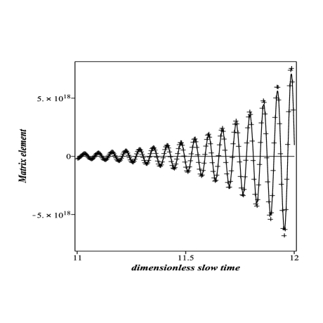
Figure 1: Numerical (points) and analytical (solid line) solutions for the matrix element $\lambda_{1}^{(11)}(t,\tau)$ in the case of $\gamma_{0}=4.0$, $\kappa_{0}=1.0$ with $\beta=2$ and $\varepsilon=0.01$.

III The photon generation from vacuum state

Knowing matrices $\Lambda(t)$ or $\mathcal{L}(t)$ (16) one can calculate immediately the time evolution of the symmetric covariance matrix $\mathcal{M}=\|\mathcal{M}_{\mu\nu}\|$, whose elements $\mathcal{M}_{\mu\nu}=\frac{1}{2}\left\langle\widehat{\mathrm{q}}_{\mu}\widehat{\mathrm{q}}_{\nu}+\widehat{\mathrm{q}}_{\nu}\widehat{\mathrm{q}}_{\mu}\right\rangle-\left\langle\widehat{\mathrm{q}}_{\mu}\right\rangle\left\langle\widehat{\mathrm{q}}_{\nu}\right\rangle$ are the central second-order statistical moments. Namely,

$$\mathcal{M}(t)=\mathcal{L}(t)\mathcal{M}(0)\widetilde{\mathcal{L}}(t).$$ (27)

For the initial vacuum states of both modes matrix $\mathcal{M}(0)$ is proportional to the unity matrix: $\mathcal{M}(0)=\frac{1}{2}I_{4}$. Consequently, in view of Eqs (16) and (27), the mean number of quanta in the $m$th mode ($m=1,2$) can be expressed in terms of diagonal elements of the sum of products of matrices $\widetilde{\lambda}_{k}$ and $\lambda_{k}$ (since the first-order mean values $\left\langle\widehat{\mathrm{q}}_{\mu}\right\rangle$ are equal to zero in the case under study):

$$\mathfrak{\bar{n}}_{m}=\frac{1}{2}\Big{(}\sum_{k=1}^{4}\widetilde{\lambda}_{k}\lambda_{k}\Big{)}^{(mm)}-\frac{1}{2}.$$ (28)

These mean numbers do not depend on the “fast time” $t$. Their explicit expressions are as follows:

$$\mathfrak{\bar{n}}_{m} =\frac{1}{4\eta^{2}}\Big{\{}\left[\eta+1+\left(1+\mathfrak{u}_{m}\right)\beta^{2}\left(\eta+\beta^{2}\right)\right]\mathbb{S}_{\mu}^{2}$$

$$+\left[\eta-1+\left(1+\mathfrak{u}_{m}\right)\beta^{2}\left(\eta-\beta^{2}\right)\right]\mathtt{S}_{\nu}^{2}$$

$$-2\beta^{2}\left(\mathbb{C}_{\mu}\mathtt{C}_{\nu}-1\right)+2\beta\mathfrak{u}_{m}\mathbb{S}_{\mu}\mathtt{S}_{\nu}\Big{\}},$$ (29)

where $\mathfrak{u}_{1}=1$ and $\mathfrak{u}_{2}=-1$. We have introduced the short notation

$$\mathbb{C}_{\mu} =\cosh(\tau_{\mu}),\qquad \mathbb{S}_{\mu}=\sinh(\tau_{\mu}),$$ (30)

$$\mathtt{C}_{\nu} =\cos(\tau_{\nu}),\qquad \mathtt{S}_{\nu}=\sin(\tau_{\nu}).$$ (31)

Typical regimes of excitations of the two modes are illustrated in Fig. 2, where we plot the photon mean numbers in the cavity mode and the detector as functions of the “dimensionless slow time” $\tau$ for different values of parameter $\beta$. Higher values of $\beta$ imply on a more intense photon generation for a given time.

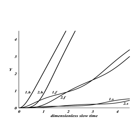
Figure 2: The behavior of function $Y(\tau)=\ln[1+\mathfrak{\bar{n}}_{m}(\tau)]$ for the cavity (1) and detector (2) with $\beta=0.2$ (s), $\beta=0.5$ (f) and $\beta=1.0$ (h). Note the time delay in increasing the number of quanta in the detector for $\beta=0.5$ and $\beta=1.0$.

We see that for $\beta=1$ the numbers of excitations in each mode grow exponentially after a short transient time, but the number of quanta in the detector mode is significantly smaller than in the cavity mode for any fixed value of $\tau$. For smaller values of $\beta$ we observe some “beats” between the two modes. However, these “beats” exist for limited time intervals, since only the first line in formula (29) is important for $\tau_{\mu}\gg 1$. Thus we see that asymptotically the number of quanta in the field mode is always bigger than in the detector (since $1+\mathfrak{u}_{1}=2$ while $1+\mathfrak{u}_{2}=0$). The ratio can be very big if $\beta\gg 1$: in this case $\mathfrak{\bar{n}}_{1}/\mathfrak{\bar{n}}_{2}\approx 4\beta^{2}=(\gamma/\kappa)^{2}$. On the other hand, $\mathfrak{\bar{n}}_{1}/\mathfrak{\bar{n}}_{2}=3$ if $\beta=1$, and $\mathfrak{\bar{n}}_{1}\approx\mathfrak{\bar{n}}_{2}$ for $\beta\ll 1$ (in the asymptotical regime $\tau_{\mu}\gg 1$).

For $\beta\ll 1$ we have $\eta\approx 1-\beta^{2}/2$, $\nu\approx 2$, and $\mu\approx\beta$, so that $\tau_{\mu}\approx\frac{1}{2}\gamma t$ and $\tau_{\nu}\approx 2\kappa t$. Therefore the numbers of excitations in the both modes coincide (provided the slow time variable $\tau$ is not very small), with corrections of the order of $\beta$:

$$\mathfrak{\bar{n}}_{m}^{(\beta\ll 1)}=\frac{1}{2}\mathbb{S}_{\mu}^{2}+\frac{\beta}{2}\mathfrak{u}_{m}\mathtt{S}_{\nu}\mathbb{S}_{\mu}+\mathcal{O}(\beta^{2}).$$ (32)

Moreover, the main term in (32) does not depend on the field-detector coupling coefficient in this case. Eq. (32) is in agreement with the results obtained in DK96 by using the method of slowly varying amplitudes (although the argument of the $\sinh$ function in DK96 was twice bigger than here due to a misprint in the definition of parameter $\mu$ in that paper).

For $\beta=1$ we have $\eta=1$, $\mu=\nu=\sqrt{2}$, and $\tau_{1}=\sqrt{2}\tau$. In this case

$$\mathfrak{\bar{n}}_{m}^{(\beta=1)}=\frac{1}{2}[\mathbb{S}_{1}^{2}+\mathbb{C}_{1}(\mathbb{C}_{1}-\mathtt{C}_{1})+\mathfrak{u}_{m}\mathbb{S}_{1}(\mathbb{S}_{1}+\mathtt{S}_{1})],$$ (33)

so that $\mathfrak{\bar{n}}_{1}^{(\beta=1)}\approx 3\mathfrak{\bar{n}}_{2}^{(\beta=1)}$ if $\tau_{1}\gg 1$.

If $\beta\gg 1$, then $\eta\approx\beta^{2}-\frac{1}{2}$, $\mu\approx 2\beta$, and $\nu\approx 1$, so that $\tau_{\mu}\approx\gamma t$ and $\tau_{\nu}\approx\kappa t$. Therefore

$$\mathfrak{\bar{n}}_{1}^{(\beta\gg 1)} =\mathbb{S}_{\mu}^{2}+\emph{O}(\beta^{-2}),$$ (34)

$$\mathfrak{\bar{n}}_{2}^{(\beta\gg 1)} =\frac{1}{4\beta^{2}}\left[\left(\mathbb{C}_{\mu}-\mathtt{C}_{\nu}\right)^{2}+2\mathtt{S}_{\nu}^{2}\right]+\emph{O}(\beta^{-3}).$$ (35)

The number of photons in the field mode coincides with the result D95 ; DK96 obtained in the absence of any detector, up to corrections of the order of $\emph{O}(\beta^{-2})$. The number of excitations in the detector is about $\beta^{2}$ times smaller, and this leads to a significant time delay in appearance of excitations in the detector: while the photons in the field mode appear after time $t_{1}\sim\gamma^{-1}$, the detector begins to “feel” their presence after the time $t_{2}\sim t_{1}\ln(\beta)$.

This time delay exists also for very small times, since in the limit $\tau\to 0$ Eq. (29) can be simplified as follows:

$$\mathfrak{\bar{n}}_{1} =4\beta^{2}\tau^{2}+\emph{O}(\tau^{4}),$$ (36)

$$\mathfrak{\bar{n}}_{2} =\beta^{2}\tau^{4}+\emph{O}(\tau^{6}).$$ (37)

IV Photon fluctuations

It is interesting to know, besides the mean numbers of quanta, their variances $\sigma_{n}=\langle\hat{n}^{2}\rangle-\langle\hat{n}\rangle^{2}$, the degree of squeezing of quadrature components and the photon distribution functions (PDF) ${\cal P}(m)\equiv\langle m|\hat{\rho}|m\rangle$, where $|m\rangle$ means the $m$th Fock state and $\hat{\rho}$ is the statistical operator describing the mixed (due to the interaction) state of the mode. For the initial vacuum states of the field mode and detector the time-dependent statistical operator is Gaussian. Therefore we can use the results obtained in Ref. VM94 for the most general Gaussian states.

IV.1 Fluctuations of the photon numbers

In our case the first-order mean values of the quadrature components are equal to zero, so that

$$\sigma_{\mathfrak{n}_{m}}=2\mathfrak{\bar{n}}_{m}^{2}+2\mathfrak{\bar{n}}_{m}-\mathcal{D}_{m}+\frac{1}{4},$$ (38)

where

$$\mathcal{D}_{m}=\mathcal{M}_{p_{m}p_{m}}\mathcal{M}_{x_{m}x_{m}}-\mathcal{M}_{x_{m}p_{m}}\mathcal{M}_{p_{m}x_{m}}$$ (39)

is the invariant uncertainty product (IUP) of the $m$th mode, which satisfies the Schrödinger–Robertson uncertainty relation QIBook $\mathcal{D}_{m}\geq 1/4$ for any quantum state. Besides, it is easy to verify that $\mathcal{D}\leq\left(\mathfrak{\bar{n}}+1/2\right)^{2}$ for the states with zero first-order mean values of the quadrature components. Therefore the variances of the photon number in the Gaussian states with zero first-order mean values of the quadrature components must obey the inequality $\sigma_{\mathfrak{n}}\geq\mathfrak{\bar{n}}\left(\mathfrak{\bar{n}}+1\right)$. The equality sign is attained for thermal (i.e., mixed) quantum states. On the other hand, for pure squeezed vacuum states with $\mathcal{D}=1/4$ we have

$$\sigma_{\mathfrak{n}}^{(sqzvac)}=2\mathfrak{\bar{n}}\left(\mathfrak{\bar{n}}+1\right).$$ (40)

The calculations lead us to the identical expressions for the functions $\mathcal{D}_{m}(t)$ for $m=1$ and $m=2$

$$\mathcal{D}_{m} =\frac{1}{4}+\frac{1}{8\eta^{4}}\Big{\{}\eta^{3}\left(\mathbb{S}_{\mu}^{2}+\mathtt{S}_{\nu}^{2}\right)-4\beta^{2}\left(\beta^{2}-1\right)\mathbb{S}_{\mu}^{2}\mathtt{S}_{\nu}^{2}$$

$$+\left(3\eta^{2}+\eta^{2}\beta^{2}-2\right)\left(\mathbb{S}_{\mu}^{2}-\mathtt{S}_{\nu}^{2}\right)-2\beta\eta^{2}\mathbb{C}_{\mu}\mathbb{S}_{\mu}\mathtt{C}_{\nu}\mathtt{S}_{\nu}$$

$$+4\beta^{3}\left(\mathbb{C}_{\mu}\mathtt{C}_{\nu}-1\right)\left(\mathbb{S}_{\mu}\mathtt{S}_{\nu}-\beta^{3}\right)\Big{\}}.$$ (41)

This result may seem surprising at first glance, since other statistical properties (such as the mean number of quanta or degree of squeezing studied in the next subsection) in each mode are different. But this is the consequence of the property of IUP for the Gaussian states: for these states IUP determines the quantum purity according to the formula $\mbox{Tr}\left(\hat{\rho}^{2}\right)=(4\mathcal{D})^{-1/2}$. On the other hand, it is known that for any pure bipartite quantum state the purities of each part are identical. Since the initial state of the total system is chosen to be pure (vacuum), it remains pure for any instant of time in the absence of dissipation (assumed in this paper). Therefore $\mathcal{D}_{1}(t)\equiv\mathcal{D}_{2}(t)$.

Simple formula for variances can be obtained if $\beta\ll 1$:

$$\sigma_{\mathfrak{n}_{m}}^{(\beta\ll 1)}=\frac{1}{4}(2\mathbb{C}_{\mu}^{2}+1)\mathbb{S}_{\mu}^{2}+\frac{\beta}{4}\mathtt{S}_{\nu}\mathbb{S}_{\mu}\mathbb{C}_{\mu}(\mathtt{C}_{\nu}+4\mathfrak{u}_{m}\mathbb{C}_{\mu}).$$ (42)

Comparing it with (32), we conclude that quantum states of the both modes are non-thermal, although they become highly mixed with the course of time, since the purity in this case diminishes as $\mbox{Tr}\left(\hat{\rho}^{2}\right)=[\cosh(\gamma t/2)]^{-1}$.

The limit (40) is achieved approximately for the field mode if $\beta\gg 1$:

$$\sigma_{\mathfrak{n}_{1}}^{(\beta\gg 1)}=2\mathbb{S}_{\mu}^{2}\mathbb{C}_{\mu}^{2}+\emph{O}(\beta^{-2}).$$ (43)

The invariant uncertainty product in this case equals

$$\mathcal{D}_{m}^{(\beta\gg 1)}=\frac{1}{4}+\frac{1}{4\beta^{2}}\left[\mathbb{C}_{\mu}^{2}+1-2\mathbb{C}_{\mu}\mathtt{C}_{\nu}\right]\left[1+\emph{O}(\beta^{-1})\right].$$ (44)

Comparing Eqs. (35) and (44), we conclude that quantum states of the both modes become significantly mixed when the mean number of excitations in the detector exceeds the unit value. For $\tau_{\mu}\gg 1$ we have $\mathcal{D}_{m}\sim\exp(2\tau_{\mu})$, whereas $\mathfrak{\bar{n}}_{m}^{2}\sim\exp(4\tau_{\mu})$. Consequently, if $\mathfrak{\bar{n}}_{m}\gg 1$, then $\sigma_{\mathfrak{n}_{m}}\approx 2\mathfrak{\bar{n}}_{m}^{2}$ for $m=1,2$, like in the squeezed vacuum state, even if the states are highly mixed.

On the other hand, the photon statistics in the two modes are quite different for $\tau_{\mu}<1$, especially in the short-time limit $\tau\to 0$. Frequently the photon statistics is characterized by the Mandel parameter $Q=\left(\sigma_{\mathfrak{n}}-\mathfrak{\bar{n}}\right)/\mathfrak{\bar{n}}$. However, in the case concerned this parameter is not very useful, since it is always greater than unity and grows unlimitedly with time in the DCE regime. A more convenient parameter is the ratio $Z_{m}\equiv\sigma_{\mathfrak{n}_{m}}/\left[\mathfrak{\bar{n}}_{m}\left(1+\mathfrak{\bar{n}}_{m}\right)\right]$, since it varies between $1$ and $2$ for the Gaussian states with zero mean values of quadrature components. The evolution of functions $Z_{1}(\tau)$ and $Z_{2}(\tau)$ for different values of parameter $\beta$ is illustrated in Fig. 3.

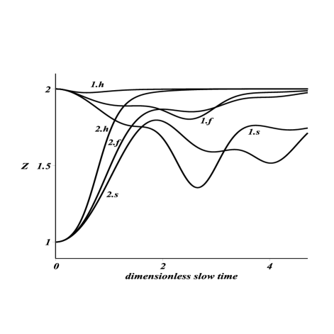
Figure 3: The time behavior of $Z_{m}\equiv\sigma_{\mathfrak{n}_{m}}/\left[\mathfrak{\bar{n}}_{m}\left(1+\mathfrak{\bar{n}}_{m}\right)\right]$ for the cavity (1) and detector (2) with $\beta=0.2$ (s), $\beta=0.5$ (f) and $\beta=1.0$ (h).

The difference is clearly seen in the limit $\tau\to 0$, when Eq. (41) can be simplified as follows:

$$\mathcal{D}_{m}(\tau)=\frac{1}{4}+\beta^{2}\tau^{4}\Big{[}1+\frac{2}{9}(3\beta^{2}-4)\tau^{2}\Big{]}+\emph{O}(\tau^{8}).$$ (45)

Therefore the contribution of $\mathcal{D}_{m}$ can be neglected in Eq. (38) with $m=1$, in view of Eq. (36), so that $Z_{1}(0)=2$. But $\mathcal{D}_{2}$ has the same order of magnitude as $\mathfrak{\bar{n}}_{2}$ for $\tau\to 0$, according to Eqs. (37) and (45). Therefore $Z_{2}(0)=1$. More precisely,

$$Z_{1}(\tau) =2-\frac{\tau^{2}}{4}\Big{[}1-\frac{5}{36}\tau^{2}\Big{]}+\frac{7}{6}\beta^{2}\tau^{4}+\emph{O}(\tau^{6}),$$

$$Z_{2}(\tau) =1+\frac{\tau^{2}}{9}\Big{[}4-\frac{19}{45}\tau^{2}\Big{]}+\frac{128}{135}\beta^{2}\tau^{4}+\emph{O}(\tau^{6}).$$

IV.2 Squeezing

The degree of squeezing is characterized by the invariant squeezing coefficient (ISC) JOBrev (which is equivalent to the principal squeezing introduced in ps )

$$\chi=\frac{4\mathcal{D}}{2\mathfrak{\bar{n}}+1+\sqrt{(2\mathfrak{\bar{n}}+1)^{2}-4\mathcal{D}}}.$$ (46)

This is twice the minimal value of variance of any quadrature component taken over the period of fast oscillations. For $\tau_{\mu}\gg 1$ we have the asymptotical formula

$$\chi_{m}^{(as)} =\mathcal{D}/\mathfrak{\bar{n}}_{m}$$

$$=\Big{[}\eta^{2}\left(\eta+\beta^{2}\right)+\left(3\eta^{2}-2\right)\mathtt{C}_{\nu}^{2}+\left(2-\eta^{2}\right)\mathtt{S}_{\nu}^{2}$$

$$-2\beta\left(\eta^{2}-2\beta^{2}\right)\mathtt{C}_{\nu}\mathtt{S}_{\nu}\Big{]}$$

$$\times\left\{2\eta^{2}\left[\beta^{2}\left(\eta+\beta^{2}\right)\left(1+\mathfrak{u}_{m}\right)+1+\eta\right]\right\}^{-1}.$$ (47)

In the special case of $\beta\ll 1$ we obtain $\chi_{m}^{(as)}=1/2$, in agreement with D95 ; DK96 . A very high degree of squeezing can be obtained in the field mode if $\beta\gg 1$: then $\chi_{1}^{(as)}=1/(4\beta^{4})$. However, there is practically no squeezing in this limit case in the detector mode: $\chi_{2}^{(as)}=1-\mathtt{C}_{\nu}\mathtt{S}_{\nu}/\beta$. For intermediate values of parameter $\beta$ the ISC does not go asymptotically to some limit value, but it exhibits slow oscillations in time with the frequency $\nu\kappa$. For example, for $\beta=1$ we obtain

$$\chi_{m}^{(as)}|_{\beta=1}=\frac{3+\sin(2\tau_{1})}{4(2+u_{m})}.$$ (48)

This function oscillates between the values $1/6$ and $1/3$ for $m=1$ (the field mode). But it is three times bigger for the detector mode. It is not difficult to calculate the minimal value of the coefficient $\chi_{2}^{(as)}$ as function of slow time $\tau_{\nu}$ for arbitrary values of parameter $\beta$:

$$\chi_{2}^{(as)}|_{min}=\frac{1}{2}+\frac{\beta(\beta-1)}{2[1+\eta(\beta)]}.$$ (49)

Moreover, the minimum of this function with respect to $\beta$ also can be found analytically. It is achieved for $\beta_{min}=(\sqrt{3}-1)/\sqrt{2}\simeq 0.52$, being equal to $(1+\sqrt{3})(\sqrt{3}-\sqrt{2})/2\simeq 0.43$. Consequently, the detector mode cannot be strongly squeezed.

IV.3 Photon distribution functions

The PDF of the Gaussian states was derived in VM94 ; Chat ; Mar . For zero mean values of quadrature components $x$ and $p$ it can be expressed in terms of the Legendre polynomials $P_{k}(x)$ as

$${\cal P}(k)=\frac{2Y_{-}^{k/2}}{Y_{+}^{(k+1)/2}}P_{k}\left(\frac{4\mathcal{D}-1}{\sqrt{Y_{+}Y_{-}}}\right),$$ (50)

where

$$Y_{\pm}=1+4\mathcal{D}\pm 2(1+2\mathfrak{\bar{n}}).$$ (51)

The behavior of PDF as function of $k$ depends on the value of the argument of the Legendre polynomial. If this argument is close to zero, then strong oscillations of function ${\cal P}(k)$ are observed, since Legendre polynomials of zero argument turn into zero for odd values of $k$. Otherwise ${\cal P}(k)$ changes slowly and monotonously. This happens for $\beta\ll 1$, as was shown in DK96 . If $\beta\gg 1$, then the argument of the Legendre polynomials for the first mode tends asymptotically to the small quantity $1/(4i\beta^{2})$, so that the PDF shows typical oscillations of the squeezed vacuum state. But for the second mode the argument of the Legendre polynomials goes asymptotically to the value $1/(i\sqrt{5})$, which is not small. Therefore the PDF of the detector mode is monotonous function without oscillations (that agrees with the absence of squeezing in this mode), which can be well approximated (for $1\ll k\sim\mathfrak{\bar{n}}$) by the universal dependence derived in D-PRA09

$${\cal P}(k)\approx\frac{\exp\left[-(2k+1)/(4\mathfrak{\bar{n}})\right]}{\sqrt{\pi\mathfrak{\bar{n}}(2k+1)}}\,.$$ (52)

In particular, considering formally $k$ as a continuous variable (i.e., using the Euler–MacLaurin summation formula), we obtain the following value for the probability of detecting any value $k$ smaller than the mean value $\bar{n}$:

$$\mbox{Prob}(k<\bar{n})=\mbox{erf}(\sqrt{2}/2)\approx 0.68,$$ (53)

where $\mbox{erf}(z)\equiv(2/\sqrt{\pi})\int_{0}^{z}\exp(-x^{2})dx$ is the error function. The distributions ${\cal P}_{1}(k)$ and ${\cal P}_{2}(k)$ for $\beta=1$ and $\tau=2$ are shown in Fig. 4. They are rather different, especially for small values of $k$. The photon mean numbers are $\mathfrak{\bar{n}}_{1}=112.4$ and $\mathfrak{\bar{n}}_{2}=38.7$. Nonetheless, the total probabilities to measure the photon number smaller than the $\mathfrak{\bar{n}}_{m}$ are practically the same for each mode: $\mbox{Prob}_{1}(k<\bar{n})=0.683$ and $\mbox{Prob}_{2}(k<\bar{n})=0.681$, in full agreement with Eq. (53).

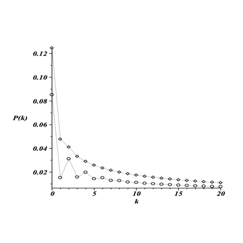
Figure 4: The photon distribution functions ${\cal P}_{m}(k)$ for the cavity $(\circ)$ and detector $(\diamond)$ in the case of $\beta=1.0$ and $\tau=2$.

V Concluding Remarks

We have shown that statistical properties of the detector quantum state (variances of the photon numbers, photon distribution function, and the degree of quadrature squeezing) can be quite different from that of the field mode. This can be important for planning the experiments on DCE and analysing their results. In particular, the discovered time delay in the increase of the mean number of quanta in the detector indicates that influence of losses in the detector (which are not taken into account in the present study) can be essential, even if losses in the cavity can be neglected. But we leave this problem for the further studies, as well as the influence of different initial states (e.g., thermal or squeezed) of the field mode and detector on the rate of generation of the Casimir photons.

Appendix A

Here we give explicit expressions for non-zero coefficients in the solutions (23) for elements of $\lambda_{k}$-matrices with $k=1$ and $k=3$.

$$F_{1}^{(11)}=\eta+\beta^{2}, \qquad G_{1}^{(12)}=-\eta+1-\beta(\beta-1),$$

$$F_{1}^{(22)}=\eta-\beta^{2}, \qquad G_{1}^{(21)}=\eta-1+\beta(\beta+1),$$

$$U_{1}^{(11)}=\eta-\beta^{2}, \qquad V_{1}^{(12)}=-\eta-1+\beta(\beta-1),$$

$$U_{1}^{(22)}=\eta+\beta^{2}, \qquad V_{1}^{(21)}=\eta+1-\beta(\beta+1),$$

$$f_{1}^{(12)}=1+\beta, \qquad g_{1}^{(11)}=\beta+1-(\beta^{2}+\eta)(2\beta+1),$$

$$f_{1}^{(21)}=-1-\beta, \qquad g_{1}^{(22)}=\beta(\beta+1)+1-\eta,$$

$$u_{1}^{(12)}=-1-\beta, \qquad v_{1}^{(11)}=(\beta^{2}-\eta)(2\beta+1)-\beta-1,$$

$$u_{1}^{(21)}=1+\beta, \qquad v_{1}^{(21)}=-\beta(\beta+1)-1-\eta,$$

$$F_{3}^{(12)}=1-\beta, \qquad G_{3}^{(11)}=1-\beta+(\beta^{2}+\eta)(2\beta-1),$$

$$F_{3}^{(21)}=\beta-1, \qquad G_{3}^{(22)}=\beta(\beta-1)+1-\eta,$$

$$U_{3}^{(12)}=\beta-1, \qquad V_{3}^{(11)}=(\eta-\beta^{2})(2\beta-1)+\beta-1,$$

$$U_{3}^{(21)}=1-\beta, \qquad V_{3}^{(22)}=-\beta(\beta-1)-1-\eta,$$

$$f_{3}^{(11)}=-\eta-\beta^{2}, \qquad g_{3}^{(12)}=\eta-1+\beta(\beta+1),$$

$$f_{3}^{(22)}=\beta^{2}-\eta, \qquad g_{3}^{(21)}=1-\eta-\beta(\beta-1),$$

$$u_{3}^{(11)}=\beta^{2}-\eta, \qquad v_{3}^{(12)}=\eta+1-\beta(\beta+1),$$

$$u_{3}^{(22)}=-\eta-\beta^{2}, \qquad v_{3}^{(21)}=\beta(\beta-1)-\eta-1.$$

All other coefficients of matrices $\lambda_{1}$ and $\lambda_{3}$ are equal to zero. The coeficients of matrices $\lambda_{2}$ and $\lambda_{4}$ are given by formulas $F_{2,4}^{(ij)}=-f_{1,3}^{(ij)}$, $f_{2,4}^{(ij)}=F_{1,3}^{(ij)}$, and similar ones for other lower case and capital symbols.

References

- (1) V. V. Dodonov, Phys. Scr. 82, 038105 (2010).
- (2) D. A. R. Dalvit, P. A. Maia Neto, and F. D. Mazzitelli, in Casimir Physics, edited by D. Dalvit, P. Milonni, D. Roberts, and F. da Rosa, Lecture Notes in Physics Vol. 834 (Springer, Berlin, 2011), p. 419.
- (3) P. D. Nation, J. R. Johansson, M. P. Blencowe, and F. Nori, Rev. Mod. Phys. 84, 1 (2012).
- (4) C. M. Wilson, G. Johansson, A. Pourkabirian, M. Simoen, J. R. Johansson, T. Duty, F. Nori, and P. Delsing, Nature 479, 376 (2011).
- (5) V. V. Dodonov, Phys. Lett. A 207, 126 (1995).
- (6) V. V. Dodonov and A. B. Klimov, Phys. Rev. A 53, 2664 (1996).
- (7) C. Braggio, G. Bressi, G. Carugno, C. Del Noce, G. Galeazzi, A. Lombardi, A. Palmieri, G. Ruoso, and D. Zanello, Europhys. Lett. 70, 754 (2005).
- (8) W.-J. Kim, J. H. Brownell, and R. Onofrio, Phys. Rev. Lett. 96, 200402 (2006).
- (9) N. B. Narozhny, A. M. Fedotov, and Yu. E. Lozovik, Phys. Rev. A 64, 053807 (2001).
- (10) T. Kawakubo and K. Yamamoto, Phys. Rev. A 83, 013819 (2011).
- (11) A. V. Dodonov, R. Lo Nardo, R. Migliore, A. Messina, and V. V. Dodonov, J. Phys. B 44, 225502 (2011).
- (12) A. V. Dodonov and V. V. Dodonov, Phys. Rev. A 85, 015805 (2012).
- (13) A. V. Dodonov and V. V. Dodonov, Phys. Rev. A 85, 055805, 063804 (2012); ibid. 86, 015801 (2012).
- (14) C. Braggio, G. Bressi, G. Carugno, F. Della Valle, G. Galeazzi, and G. Ruoso, Nucl. Instr. and Meth. A 603, 451 (2009).
- (15) A. V. Dodonov and V. V. Dodonov, Phys. Lett. A 376, 1903 (2012).
- (16) V. V. Dodonov and V. I. Man’ko, Invariants and the Evolution of Nonstationary Quantum Systems, edited by M. A. Markov, Proceedings of Lebedev Physics Institute Vol. 183 (Nova Science, Commack, New York, 1989).
- (17) A. H. Nayfeh and D. T. Mook, Nonlinear Oscillations (John Wiley and Sons, New York, 1995).
- (18) M. Janowicz, Phys. Rep. 375, 327 (2003).
- (19) V. V. Dodonov, O. V. Man’ko, and V. I. Man’ko, Phys. Rev. A 49, 2993 (1994).
- (20) V. V. Dodonov, J. Opt. B 4, R1 (2002).
- (21) A. Lukš, V. Peřinová, and Z. Hradil, Acta Phys. Polon. A 74, 713 (1988).
- (22) S. Chaturvedi and V. Srinivasan, Phys. Rev. A 40, 6095 (1989).
- (23) P. Marian, Phys. Rev. A 45, 2044 (1992).
- (24) V. V. Dodonov, Phys. Rev. A 80, 023814 (2009).