Model Checking of Linear-Time Properties in Multi-Valued Systems

Abstract

In this paper, we study the model-checking problem of linear-time properties in multi-valued systems. Safety properties, invariant properties, liveness properties, persistence and dual-persistence properties in multi-valued logic systems are introduced. Some algorithms related to the above multi-valued linear-time properties are discussed. The verification of multi-valued regular safety properties and multi-valued $\omega$-regular properties using lattice-valued automata are thoroughly studied. Since the law of non-contradiction (i.e., $a\wedge\neg a=0$) and the law of excluded-middle (i.e., $a\vee\neg a=1$) do not hold in multi-valued logic, the linear-time properties introduced in this paper have new forms compared to those in classical logic. Compared to those classical model-checking methods, our methods to multi-valued model checking are accordingly more direct: We give an algorithm for showing $TS\models P$ for a model $TS$ and a linear-time property $P$, which proceeds by directly checking the inclusion $Traces(TS)\subseteq P$ instead of $Traces(TS)\cap\neg P=\emptyset$. A new form of multi-valued model checking with membership degree is also introduced. In particular, we show that multi-valued model checking can be reduced to classical model checking. The related verification algorithms are also presented. Some illustrative examples and a case study are also provided.

1 Introduction

In the last four decades, computer scientists have systematically developed theories of correctness and safety as well as methodologies, techniques and even automatic tools for correctness and safety verification of computer systems; see for example [34, 42, 1]. Of which, model checking has become established as one of the most effective automated techniques for analyzing correctness of software and hardware designs. A model checker checks a finite-state system against a correctness property expressed in a propositional temporal logic such as LTL (Linear Temporal Logic) or CTL (Computational Tree Logic). These logics can express safety (e.g., “No two processes can be in the critical section at the same time”) and liveness (e.g., “Every job sent to the printer will eventually print”) properties. Model checking has been effectively applied to reasoning about correctness of hardware, communication protocols, software requirements, etc. Many industrial model checkers have been developed, including SPIN [25], SMV [43].

Despite their variety, existing model checkers are typically limited to reasoning in classical logic. However, there are a number of problems for which classical logic is insufficient. One of these is reasoning under uncertainty. This can occur either when complete information is not known or cannot be obtained (e.g., during ‘requirements’ analysis), or when this information has been removed (abstraction). Classical model checkers typically deal with uncertainty by creating extra states, one for each value of the unknown variable and each feasible combination of values of known variables. However, this approach adds significant extra complexity to the analysis. Classical reasoning is also insufficient for models that contain inconsistencies. Models may be inconsistent because they combine conflicting points of view, or because they contain components developed by different people. Conventional reasoning systems cannot cope with inconsistency because the presence of a single contradiction results in trivialization – anything follows from $A\wedge\neg A$. Hence, faced with an inconsistent description and the need to perform automated reasoning, we must either discard information until consistency is achieved again, or adopt a nonclassical logic. Multi-valued logic (mv-logic, in short) provides a solution to both reasoning under uncertainty and under inconsistency. For example, we can use unknown and no agreement as logic values. In fact, model checkers based on three-valued and four-valued logics have already been studied. For example, [8] (c.f., [45]) used a three-valued logic for interpreting results of model-checking with abstract interpretation, whereas [24] used four-valued logics for reasoning about abstractions of detailed gate or switch-level designs of circuits. For reasoning about dynamic properties of systems, we need to extend existing modal logics to the multi-valued case. Fitting [20] explores two different approaches for doing this: the first extends the interpretation of atomic formulae in each world to be multi-valued; the second also allows multi-valued accessibility relations between worlds. The latter approach is more general, and can readily be applied to the temporal logics used in model checking [12]. We use different multi-valued logics to support different types of analysis. For example, to model information from multiple sources, we may wish to keep track of the origin of each piece of information, or just the majority vote, etc. Thus, rather than restricting ourselves to any particular multi-valued logic, our approach is to extend classical symbolic model checking to arbitrary multi-valued logics, as long as conjunction, disjunction and negation of the logical values are well defined. M. Chechik and her colleagues have published a series of papers along this line, see [8, 9, 10, 12, 13].

Our purpose is to develop automata-based model-checking techniques in the multi-valued setting. More precisely, the major design decision of this paper is as follows:

A lattice-valued automaton is adopted as the model of the systems. This is reasonable since classical automata (or equivalent transition systems) are common system models in classical model checking. Linear-time properties of multi-valued systems are checked in this paper. They are defined to be infinite sequences of sets of atomic propositions, as in the classical case, with truth-values in a given lattice. The key idea of the automata-based approach to model checking is that we can use an auxiliary automaton to recognize the properties to be checked, and then combine it with the system to be checked so that the problem of checking the safety or $\omega$-properties of the system is reduced to checking some simpler (invariance or persistence) properties of the larger system composed by the systems under checking and the auxiliary automaton. A difference between the classical case and the multi-valued case deserves a careful explanation. Since the law of non-contradiction (i.e., $a\wedge\neg a=0$) and the law of excluded middle (i.e., $a\vee\neg a=1$) do not hold in multi-valued logic, the present forms of many classical properties in multi-valued logic must have some new forms, and some distinct constructions need to be given in multi-valued logic.

As said in Ref. [2], the equivalences and preorders between transition systems that “correspond” to linear temporal logic are based on trace inclusion and equality, whereas for branching temporal logic such relations are based on simulation and bisimulation relations. That is to say, the model checking of a transition system $TS$ which represents the model of a system satisfying a linear temporal formula $\varphi$, i.e., $TS\models\varphi$ is equivalent to checking the inclusion relation $Traces(TS)\subseteq P$, where $Traces(TS)$ is the trace function of the transition system $TS$ and $P$ is the temporal property representing the formula $\varphi$. In classical logic, we know that $a\leq b$ if and only if $a\wedge\neg b=0$ holds. Therefore, $TS\models\varphi$ if and only if $Traces(TS)\cap\neg P=\emptyset$. Then, instead of checking $TS\models\varphi$ directly using the inclusion relation $Traces(TS)\subseteq P$, it is equivalent to checking the emptiness of the language $L({\cal A})\cap L({\cal A}_{\neg\varphi})$ indirectly, where ${\cal A}$ is a Büchi automaton representing the trace function of the transition system $TS$ (i.e., $L({\cal A})=Traces(TS))$, and ${\cal A}_{\neg\varphi}$ is a Büchi automaton related to temporal property $\neg\varphi$ (i.e., $L({\cal A}_{\neg\varphi})=\neg P$).

In contrast, in mv-logic, $a\leq b$ is in general not equivalent to the condition $a\wedge\neg b=0$, so the classical method to solve model checking of linear-time properties does not universally apply to the multi-valued model checking. The available methods of multi-valued model checking ([9]) still used the classical method with some minor correction. That is, instead of checking of $TS\models P$ for a multi-valued linear time property $P$ using the inclusion of the trace function $Traces(TS)\subseteq P$, the available method only checked the membership degree of the language $L({\cal A})\cap L({\cal A}_{\neg P})$, where ${\cal A}_{\neg P}$ is a multi-valued Büchi automaton such that $L({\cal A}_{\neg P})=\neg P$. As we know, these two methods are not equivalent in mv-logic. Then, some new methods to apply multi-valued model checking of linear-time properties based on trace inclusion relations need to be developed.

We provide new results along this line. In fact, we shall give a method of multi-valued model checking of linear-time property directly using the inclusion of the trace function of $TS$ into a linear-time property $P$. In propositional logic, we know that we can use the implication connective $\rightarrow$ to represent the inclusion relation. In fact, in classical logic, we know that the implication connective can be represented by disjunction and negation connectives, that is, $a\rightarrow b=\neg a\vee b$. In this case, we know that $a\leq b$ if and only if $\neg a\vee b=1$, if and only if $a\wedge\neg b=0$, if and only if $a\rightarrow b=1$. Then a natural problem arises: how to define the implication connective in multi-valued logic? By the above analysis, it is not appropriate to use the implication connective defined in the form $a\rightarrow b=\neg a\vee b$ to represent the inclusion relation in multi-valued logic. In order to use the implication connective to reflect the inclusion relation in mv-logic, we shall use implication connective $\rightarrow$ as a primitive connective in multi-valued logic as done in [23]. In this case, we will have that $a\leq b$ is equivalent to $a\rightarrow b=1$ semantically. Then we can use the implication connective to present the inclusion relation in multi-valued logic. This view will give a new idea to study linear-time properties in multi-valued model checking. Furthermore, we also show that we can use the classical model checking methods (such as SPIN and SMV) to solve the multi-valued model-checking problem. In particular, some special and important multi-valued linear-time properties are introduced, which include safety, invariance, persistence and dual-persistence properties, and the related verification algorithms are also presented. In multi-valued systems, the verification of the mentioned properties require some different structures compared to their classical counterpart. In particular, since the law of non-contradiction and the law of excluded middle do not hold in multi-valued logic, the auxiliary automata used in the verification of multi-valued regular safety properties and multi-valued $\omega$-regular properties need to be deterministic, whereas nondeterministic automata suffice for the classical cases.

There are at least two advantages of the method used in this paper. First, we use the implication connective as a primitive connective which can reflect the “trace inclusion” in multi-valued logic, i.e., in multi-valued model checking, $TS\models P$ if and only if $Trace(TS)\subseteq P$, the natural corresponding counterpart in multi-valued logic is, $a\leq b$ if and only if $a\rightarrow b=1$. Second, since there is a well-established multi-valued logic frame using the implication connective as a primitive connective ([23]), there will be a nice theory of multi-valued model checking, especially, model checking of linear-time property in mv-logic. Of course, this approach can be seen as another view on the study of multi-valued model checking.

The content of this paper is arranged as follows. We first recall some notions and notations in multi-valued logic systems in Section 2. In Section 3, the multi-valued linear-time properties are introduced. In particular, the notions of multi-valued regular safety properties and multi-valued liveness properties are introduced, then the reduction of model checking of multi-valued invariant properties into classical ones is presented. The verification of multi-valued regular safety properties is discussed in Section 4. In Section 5, the verification of multi-valued $\omega$-regular properties is developed. Some general considerations about the multi-valued model checking are discussed in Section 6, in which the truth-valued degree of an mv-transition system satisfying a multi-valued linear-time property is introduced. Examples and a case study illustrating the method of this article are presented in Section 7. The summary, comparisons and the future work are included in the conclusion part. We place the proofs of some propositions of this article in the Appendix parts for readability.

2 Multi-valued logic: some preliminaries

Let us first recall some notions and notations of multi-valued logic, which can be found in the literature [3, 10, 4, 23]. We start by presenting ordered sets and lattices which play a very important role in multi-valued logic.

Definition 1.

A partial order, $\leq$, on a set $l$ is a binary relation on $l$ such that for all $x,y,z\in l$ the fo1lowing conditions hold:

(1) (reflexivity) $x\leq x$.

(2) (anti-symmetry) $x\leq y$ and $y\leq x$ imply $x=y$.

(3) (transitivity) $x\leq y$ and $y\leq z$ imply $x\leq z$.

A partially ordered set, $(l,\leq)$, has a bottom (or the least) element if there exists $0\in l$ such that $0\leq x$ for any $x\in l$. The bottom element is also denoted by $\bot$. Dually, $(l,\leq)$ has a top (or the largest) element if there exists $1\in l$ such that $x\leq 1$ for all $x\in l$. The top element is also denoted as $\top$.

Definition 2.

A partially ordered set, $(l,\leq)$, is a lattice if the greatest lower bound and the least upper bound exist for any nonempty finite subset of $l$.

Given lattice elements $a$ and $b$, their greatest lower bound is referred to as meet and denoted $a\wedge b$, and their least upper bound is referred to as join and denoted $a\vee b$. By Definition 2, a lattice $(l,\leq)$ is called bounded if it contains a top element $1$ and a bottom element $0$.

Remark 1.

A complete lattice is a partially ordered set, $(l,\leq)$, in which the greatest lower bound and the least upper bound exist for any subset of $l$. For a subset $X$ of $l$, its greatest lower bound and least upper bound are denoted by $\bigwedge X$ or $\bigvee X$, respectively. Any complete lattice is bounded, since $1=\bigwedge\emptyset$ and $0=\bigvee\emptyset$.

Definition 3.

A lattice $l$ is distributive if and only if one of the following (equivalent) distributivity laws holds,

$x\wedge(y\vee z)=(x\wedge y)\vee(x\wedge z)$,

$x\vee(y\wedge z)=(x\vee y)\wedge(x\vee z)$.

The join-irreducible elements are crucial for the use of distributive lattices in this article.

Definition 4.

Let $l$ be a lattice. Then an element $x\in l$ is called join-irreducible if $x\not=0$ and $x=y\vee z$ implies $x=y$ or $x=z$ for all $y,z\in l$.

If $l$ is a distributive lattice, then a non-zero element $x$ in $l$ is join-irreducible iff $x\leq y\vee z$ implies that $x\leq y$ or $x\leq z$ for any $y,z\in l$. We use $JI(l)$ to denote the set of join-irreducible elements in $l$. It is well-known that $l$ is generated by its join-irreducible elements if $l$ is a finite distributive lattice, that is, for any $a\in l$, there exists a finite subset $A$ of $JI(l)$ such that $a=\bigvee A$. In other words, every element of $l$ can be written as the join of finitely many join-irreducible elements.

Furthermore, we present the definition of de Morgan algebra, also called quasi-Boolean algebra as in [10].

Definition 5.

A de Morgan algebra is a tuple $(l,\leq,\wedge,\vee,\neg,0,1)$, such that $(l,\leq,\wedge,\vee,0,1)$ is a bounded distributive lattice, and the negation $\neg$ is a function $l\rightarrow l$ such that $x\leq y$ implies $\neg y\leq\neg x$ and $\neg\neg x=x$ for any $x,y\in l$. Then $\neg x$ is also called the (quasi-)complement of $x$.

In a de Morgan algebra, the de Morgan laws hold, that is, $\neg(x\vee y)=\neg x\wedge\neg y$ and $\neg(x\wedge y)=\neg x\vee\neg y$. Also, $\neg 0=1$ and $\neg 1=0$. It is well-known that a Boolean algebra is a de Morgan algebra $B$ with the additional conditions that for every element $x\in B$,

Law of Non-Contradiction:   $x\wedge\neg x=0$.

Law of Excluded Middle:      $x\vee\neg x=1$.

Example 2.

In Fig. 1, we present some examples of de Morgan algebras, where $B_{2}$, $l_{3}$ and $l_{5}$ are linear orders.

(1) The lattice $B_{2}$ in Fig.1, with $\neg 0=1$ and $\neg 1=0$, gives us classical logic.

(2) The three-valued logic $l_{3}$ is defined in Fig.1, where $\neg$F=T, $\neg$M=M and $\neg$T=F.

(3) The lattice $B_{2}\times B_{2}$ in Fig.1 shows the product algebra, where $\neg(0,0)=(1,1)$, $\neg(1,0)=(0,1)$, $\neg(0,1)=(1,0)$ and $\neg(1,1)=(0,0)$. This logic can be used for reasoning about disagreement between two knowledge sources.

(4) The lattice $l_{5}$ in Fig.1 shows a five-valued logic and possible interpretations of its value as, T=Definitely true, L=Likely or weakly true, M=Maybe or unknown, U=Unlikely or weakly false, and F=Definitely false, where $\neg$T=F, $\neg$L=U, $\neg$M=M, $\neg$U=L, and $\neg$F=T.

(5) The lattice $l_{3}\times l_{3}$ in Fig.1 shows a nine-valued logic constructed as the product algebra. Like $B_{2}\times B_{2}$, this logic can be used for reasoning about disagreements between two sources, but also allows missing information in each source.

Figure 1: Some lattices

In the following, we always assume that $l$ is a de Morgan algebra, and it is also called an algebra.

Given an algebra $l$, we now can define multi-valued sets and multi-valued relations, which are functions taking values in $l$. Multi-valued sets and multi-valued relations are basic data structures in multi-valued model checking introduced later in this paper.

Definition 6.

Given an algebra $l$ and a classical set $X$, an $l$-valued set on $X$, referred to as $f$, is a function $X\rightarrow l$.

The collection of all $l$-sets on $X$ is denoted $l^{X}$, called the $l$-power set of $X$.

When the underlying algebra $l$ is clear from the context, we refer to an $l$-valued set just as multi-valued set (mv-set, for short). For an mv-set $f$ and an element $x$ in $X$, we will use $f(x)$ to define the membership degree of $x$ in $f$. In the classical case, this amounts to representing a set by its characteristic function.

The standard operations on mv-sets $f,g$ are defined in the following manner:

mv-intersection: $(f\cap g)(x)\triangleq f(x)\wedge g(x)$.

mv-union: $(f\cup g)(x)\triangleq f(x)\vee g(x)$.

set inclusion: $f\subseteq g\triangleq\forall x.(f(x)\leq g(x))$.

extensional equality: $f=g\triangleq\forall x.(f(x)=g(x))$.

mv-complement: $\neg f(x)\triangleq\neg(f(x))$.

Definition 7.

For a given algebra $l$, an $l$-valued relation $R$ on two sets $X$ and $Y$ is an $l$-valued set on $X\times Y$.

For any $l$-valued set $f:X\rightarrow l$, and for any $m\in l$, the $m$-cut of $f$ is defined as the subset $f_{m}$ of $X$ with

$f_{m}=\{x\in X|f(x)\geq m\}$.

The support of $f$, denoted by $supp(f)$, is the following subset of $X$,

$supp(f)=\{x\in X|f(x)>0\}$.

Then we have a resolution of $f$ by its cuts presented in the following proposition.

Proposition 3.

For any $l$-valued set $f:X\rightarrow l$, we have

$f=\bigcup_{m\in l}m\wedge f_{m}$,

where $m\wedge f_{m}$ is an $l$-valued set defined as $m\wedge f_{m}(x)=m$ if $x\in f_{m}$ and $0$ otherwise. Furthermore, if $l$ is finite, then

$f=\bigcup_{m\in JI(l)}m\wedge f_{m}$.

The verification is simple, we omit its proof here. As a corollary, we have the following proposition.

Proposition 4.

Given two $l$-valued sets $f,g:X\rightarrow l$, $f\leq g$ if and only if $f_{m}\subseteq g_{m}$ for every $m\in l$. Furthermore, if $l$ is finite, $f\leq g$ if and only if $f_{m}\subseteq g_{m}$ for every $m\in JI(l)$.

In order to define the semantics of multi-valued implication, we will need the algebra $l$ to have an implication operator. There are at least two methods to define the implication operator. First, it can be defined by other primitive connectives in mv-logic logic. For example, we can use $a\rightarrow b=\neg a\vee b$ as a material implication or $a\rightarrow b=\neg a\vee(a\wedge b)$ as a quantum logic implication to define the implication operator. In fact, in Ref.[10, 9], the implication operator is chosen as the material implication. The second choice of implication operator is as a primitive connective in $l$ that satisfies the condition $a\rightarrow b=1$ whenever $a\leq b$. In this paper, we shall use the second method to define the implication operator. We shall give some analysis of our choice in Section 6. Then we need $l$ to be a residual lattice or Heyting algebra defined as follows.

Definition 8.

Let $l$ be a bounded lattice and $\rightarrow$ a binary function on $l$ such that for any $a,b\in l$, the element $a\rightarrow b=\rightarrow(a,b)$ in $l$ satisfies the following condition,

$x\leq a\rightarrow b$ iff $x\wedge a\leq b$,

for any $x\in l$. Then $l$ is called a residual lattice or Heyting algebra, and the operator $\rightarrow$ is called the implication or the residual operator in $l$.

For example, if $l$ is a linear order, then $a\rightarrow b=1$ if $a\leq b$ and $a\rightarrow b=b$ if $a>b$; if $l$ is a Boolean algebra, then $a\rightarrow b=\neg a\vee b$. In particular, each finite distributive lattice is a residual lattice. Note that in any residual lattice, we have $a\rightarrow b=1$ iff $a\leq b$.

Any complete lattice $l$ satisfying the infinite distributive law, i.e.,

$x\wedge(\bigvee_{i\in I}a_{i})=\bigvee_{i\in I}(x\wedge a_{i})$,

is a residual lattice, and the implication operator is defined as follows,

$a\rightarrow b=\bigvee\{c\in l|a\wedge c\leq b\}$.

The algebra $l$ in this paper is required to be a residual lattice. This is the main difference of our method from those used in [8, 9, 12, 10, 13]. We shall give some analysis why we use the implication operator in the second form in Section 6.

Remark 5.

As ordered structures we take Heyting algebras which are de Morgan algebras, i.e., bounded lattices which have an residual operator $\rightarrow$ and a self-inverse negation operation. It is known from lattice theory that there are many Heyting and de Morgan algebras which are not Boolean algebras, cf., e.g., [22]. For instance, any finite linear order is a Heyting and de Morgan algebra but not a Boolean algebra (if it has more than 2 elements). Other examples of Heyting algebras occur e.g. in intuitionistic logic and in pointless topology studied for denotational semantics of programming languages.

With these preliminaries, we can introduce some simple facts about multi-valued logic (mv-logic, in short).

Similar to that of classical first-order logic, the syntax of multi-valued or $l$-valued logic has three primitive connectives $\vee$ (disjunction), $\neg$ (negation) and $\rightarrow$ (implication), and one primitive quantifier $\exists$ (existential quantifier). In addition, we need to use some set-theoretical formulas. Let $\in$ (membership) be a binary (primitive) predicate symbol. Then $\subseteq$ and $\equiv$ (equality) can be defined with $\in$ as usual. The semantics of multi-valued logic is given by interpreting the connectives $\vee$ and $\neg$ as the operations $\vee$ and $\neg$ on $l$, respectively, and interpreting the quantifier $\exists$ as the least upper bound in $l$. Moreover, the truth value of the set-theoretical formula $x\in A$ is $[x\in A]=A(x)$. In multi-valued logic, $1$ is the unique designated truth value; a formula $\varphi$ is valid iff $[\varphi]=1$, and denoted by $\models_{l}\varphi$.

In this article, we only use multi-valued proposition formulae. We give their formal definition here.

Definition 9.

Given a set of atomic propositions $AP$, the multi-valued proposition formulae (mv-proposition formulas, in short) generated by $AP$ are defined by the following BNF expression:

$\varphi:=A|r|\varphi_{1}\vee\varphi_{2}|\neg\varphi|\varphi_{1}\rightarrow\varphi_{2},$

where $r\in l$ and $A\in AP$.

The set of mv-proposition formulae is denoted by $l$-$AP$.

We can define conjunction and equivalence as usual,

$\varphi_{1}\wedge\varphi_{2}=\neg(\neg\varphi_{1}\vee\neg\varphi_{2})$ and $\varphi_{1}\leftrightarrow\varphi_{2}=(\varphi_{1}\rightarrow\varphi_{2})\wedge(\varphi_{2}\rightarrow\varphi_{1})$.

For any valuation of atomic propositions $v:AP\rightarrow l$, the truth-value of an mv-proposition formula $\varphi$ under $v$ is an element in $l$, denoted $v(\varphi)$, which is defined inductively as follows,

$v(\varphi)=v(A)$ if $\varphi=A\in AP$;

$v(\varphi)=r$ if $\varphi=r\in l$;

$v(\varphi_{1}\vee\varphi_{2})=v(\varphi_{1})\vee v(\varphi_{2})$;

$v(\neg\varphi)=\neg v(\varphi)$;

$v(\varphi_{1}\rightarrow\varphi_{2})=v(\varphi_{1})\rightarrow v(\varphi_{2})$.

For a set of proposition formulae $\Phi\subseteq AP$, the characterization function of $\Phi$ is a valuation $v$ on $AP$ such that $v(A)=1$ if $A\in\Phi$ and $0$ otherwise. In this case, we write $v(\varphi)$ as $\varphi(\Phi)$.

Multi-valued temporal logic formulae have also been defined in the literature. For further reading, we refer to [10].

3 Linear-time properties in multi-valued systems

In this section, we shall introduce several notions of linear-time properties in mv-logic, including multi-valued version of safety, invariance, persistence, dual persistence, and liveness. As starting point, let us first give the notion of multi-valued transition system, which is used to model the system under consideration.

3.1 Multi-valued transition systems and their trace functions

Transition systems or Kripke structures are the key models for model checking. Corresponding to multi-valued model checking, we have the notion of multi-valued transition systems, which are defined as follows (for the notion of multi-valued Kripke structures, we refer to [10]).

Definition 10.

A multi-valued transition system (mv-TS, for short) is a 6-tuple $TS=(S,Act,\eta,I,AP,L)$, where

(1) $S$ denotes a set of states;

(2) $Act$ is a set of the names of actions;

(3) $\eta:S\times Act\times S\rightarrow l$ is an mv-transition relation;

(4) $I:S\rightarrow l$ is mv-initial state;

(5) $AP$ is a set of (classical) atomic propositions;

(6) $L:S\rightarrow 2^{AP}$ is a labeling function.

$TS$ is called finite if $S$, $Act$,and $AP$ are finite.

We always assume that an mv-TS is finite in this paper.

Here, the labeling function $L$ is the same as in the classical case. In Ref.[10], it required that the labeling function is also multi-valued, that is, $L$ is a function from the states set $S$ into $l^{AP}$. We shall show that they are equivalent as trace functions in Appendix A.

For convenience, we use $(s,\alpha,s^{\prime},r)\in\rightarrow$ to represent $\eta(s,\alpha,s^{\prime})=r$, and the $TS=(S,Act,\eta,I,AP,L)$ is denoted by $TS=(S,Act,\rightarrow,I,AP,L)$ in the following. Intuitively, $\eta(s,\alpha,s^{\prime})$ stands for the truth value of the proposition that action $\alpha$ causes the current state $s$ to become the next state $s^{\prime}$. The intuitive behavior of an mv-transition system can be described as follows. The transition system starts in some initial state $s_{0}\in I$ (in multi-valued logic) and evolves according to the transition relation $\rightarrow$. That is, if $s$ is the current state, then a transition $(s,\alpha,s^{\prime},r)\in\rightarrow$ originating from $s$ is selected in the mv-logic sense and taken, i.e., the action $\alpha$ is performed and the transition system evolves from state $s$ into state $s^{\prime}$ with truth value $r$. This selection procedure is repeated in state $s^{\prime}$ and finishes once a state is encountered that has no outgoing transitions. (Note that $I$ may be empty; in that case, the transition system has no behavior at all as no initial state can be selected.) It is important to realize that in case a state has more than one outgoing transition, the next transition is chosen in a purely mv-logic fashion. That is, the outcome of this selection process is known with some truth-value a priori, and, hence, the degree with which a certain transition is selected is given a priori in the mv-logic sense.

Let $TS=(S,Act,\rightarrow,I,AP,L)$ be a transition system. A finite execution fragment (or a run) $\varrho$ of TS is an alternating sequence $\varrho=s_{0}\alpha_{1}s_{1}\alpha_{2}...\alpha_{n}s_{n}$ of states and actions ending with a state. If $\eta(s_{i},\alpha_{i+1},s_{i+1})=r_{i+1}$ for all $0\leq i<n$, where $n\geq 0$, the sequence has truth value $v(\varrho)=I(s_{0})\wedge r_{1}\wedge r_{2}\wedge\cdots\wedge r_{n}$. We refer to $n$ as the length of the execution fragment $\varrho$. An infinite execution fragment $\rho$ of $TS$ is an infinite, alternating sequence of states and actions: $\rho=s_{0}\alpha_{1}s_{1}\alpha_{2}...$, and if $\eta(s_{i},\alpha_{i+1},s_{i+1})=r_{i+1}$ for all $0\leq i$, the sequence has truth value $v(\rho)=I(s_{0})\wedge r_{1}\wedge r_{2}\wedge\cdots=\bigwedge_{i\geq 0}r_{i}$, where $r_{0}=I(s_{0})$.

For a finite execution fragment $\varrho$ or an infinite execution fragment $\rho$ of $TS$, the corresponding finite sequence or infinite sequence of states, denoted $\pi(\varrho)=s_{0}s_{1}\cdots s_{n}$ or $\pi(\rho)=s_{0}s_{1}\cdots$, respectively, is called the path of $TS$ corresponding to $\varrho$ or $\rho$.

In general, an infinite path or a computation of an mv-TS, $TS$, is an infinite sequence of states (i.e., $s_{0}s_{1}\cdots$) such that $s_{0}\in I$ and $\eta(s_{i},\alpha_{i},s_{i+1})>0$ for some $\alpha_{i}$. In order to describe an infinite sequence of states, we will use the function $\pi:{\bf N}\rightarrow S$ defined as: $\pi(i)$ is the i-th state in the sequence $s_{0}s_{1}\cdots$. In the following, $\pi$ will denote a path of the mv-TS and $\pi[i]$ will denote the actual sequence of states, that is, $\pi[i]=\pi(i)\pi(i+1)\cdots$. We use $\overline{\pi}$ to denote a finite fragment of $\pi$.

Let $TS=(S,Act,\rightarrow,I,AP,L)$ be an mv-TS, then for each $s\in S$,

$Paths_{TS}(s)=\{\pi:{\bf N}\rightarrow S|(\pi(0)=s)(\forall i\in{\bf N})(\exists\alpha_{i}\in Act)(\eta(\pi(i),\alpha_{i},\pi(i+1))>0)\}$,

which is the set of all infinite paths starting at state $s$.

For $T\subseteq S$, we write $Paths_{TS}(T)=\bigcup_{s\in T}Paths_{TS}(s)$. Let $Paths(TS)=Paths_{TS}(S)$.

Also, we define $S_{inf}=\{s\in S|Paths_{TS}(s)\not=\emptyset\}$. If the transition relation $\rightarrow$ is total, that is, for all $s\in S$, there exists $\alpha\in Act$ and $s^{\prime}\in S$ such that $\eta(s,\alpha,s^{\prime})>0$, then we also call this $TS$ without terminal state. In this case, $S_{inf}=S$.

A trace is the sequence of labelings (or observations) corresponding to a path $\pi$, $L(\pi(0))L(\pi(1))\cdots$ which will be again denoted by $L(\pi)$ or $trace(\pi)$. The definition of the trace as function will be the composition of the map $L$ and $\pi$, i.e., the map $L\circ\pi:{\bf N}\rightarrow 2^{AP}$. The $l$-language or multi-valued language (mv-language, in short) of the transition system $TS$ over $2^{AP}$, which is also called the multi-valued trace function of $TS$, is defined as the function $Traces(TS)$ from $(2^{AP})^{\omega}$ into $l$ as follows,

$Traces(TS)(\sigma)=\bigvee\{v(\rho)|L(\pi(\rho))=\sigma\}$.

Observe that this supremum exists since by assumption $TS$ is finite, hence $v$ has finite image. In fact, $Traces(TS)$ registers sequences of the set of atomic propositions $L(\pi)$ that are valid along the execution with truth value $Traces(TS)(L(\pi))$.

A multi-valued trace function $Traces(TS):(2^{AP})^{\omega}\rightarrow l$ is a multi-valued linear-time property over $2^{AP}$ defined in general as follows.

Definition 11.

An mv-linear-time property (LT-property, in short) $P$ over the set of atomic propositions $AP$ is an mv-subset of $(2^{AP})^{\omega}$, i.e., $P:(2^{AP})^{\omega}\rightarrow l$.

LT properties specify the traces that an mv-TS should exhibit. Informally speaking, one could say that an LT property specifies the admissible (or desired) behavior of the system under consideration.

The fulfillment of an LT property by an mv-TS is defined as follows.

Definition 12.

For an mv-TS, $TS$, and an mv-linear-time property $P$, we let $TS\models P$ if $Traces(TS)\subseteq P$.

In mv-logic, even if $TS\models P$ does not hold, i.e., $Traces(TS)\subseteq P$ does not hold, we still have the membership degree of the inclusion relation, denoted $lMC(TS,P)$, which presents the degree of the inclusion of $Traces(TS)$ in $P$. The study of $lMC(TS,P)$ is more general and complex, so we will discuss it only in Section 6.

In the following, we will define several mv-linear-time properties including safety and liveness properties.

3.2 Multi-valued safety property

Safety properties are often characterized as “nothing bad should happen”. Formally, in the classical case, a safety property is defined as an LT property over $AP$ such that any infinite word $\sigma$ where $P$ does not hold contains a bad prefix. Since it is difficult to define the notion of bad prefix in the mv-logic, we use the dual notion of good prefixes to define the multi-valued safety property here. Of course, they are equivalent in the classical case. We need $l$ to be complete in the following.

Definition 13.

For an mv-linear-time property $P:(2^{AP})^{\omega}\rightarrow l$, define an mv-language $GPref(P):(2^{AP})^{\ast}\rightarrow l$ as,

$GPref(P)(\theta)=\bigvee\{P(\theta\tau)|\tau\in(2^{AP})^{\omega}\}$

for any $\theta\in(2^{AP})^{\ast}$. We call $GPref(P)$ the mv-language of good prefixes of $P$.

The closure $Closure(P)$ of $P$ is the mv-linear-time property over $(2^{AP})^{\omega}$ defined as follows,

$Closure(P)(\sigma)=\bigwedge\{GPref(P)(\theta)|\theta\in Pref(\sigma)\}$,

for any $\sigma\in(2^{AP})^{\omega}$, where $Pref(\sigma)=\{\theta\in(2^{AP})^{\ast}|\sigma=\theta\sigma^{\prime}$ for some $\sigma^{\prime}\in(2^{AP})^{\omega}\}$ is called the prefix set of $\sigma$.

$P$ is called a safety property if

$Closure(P)\subseteq P$.

Informally, an mv-safety property can be characterized as “anything always good must happen”, which is equivalent to the saying “nothing bad should happen”.

An mv-safety property can be characterized by a closure operator which is formally defined as follows.

Proposition 6.

For mv-linear-time properties $P,P_{1}$ and $P_{2}$, we have

(1) $P\subseteq Closure(P)$;

(2) If $Im(P_{1})$ and $Im(P_{2})$ are finite subsets of $l$, then $Closure(P_{1}\cup P_{2})=Closure(P_{1})\cup Closure(P_{2})$;

(3) $Closure(Closure(P))=Closure(P)$;

(4) $Closure(P)$ is the smallest safety property containing $P$, i.e., $Closure(P)$ is a safety property and if $Q$ is a safety property with $P\subseteq Q$, then $Closure(P)\subseteq Q$.

The proof is placed in Appendix B.

The following is immediately by Proposition 6(1) and the definition of safety property.

Proposition 7.

For an mv-linear-time property $P$, $P$ is a safety property if and only if $P=Closure(P)$.

Given $TS$, we define the finite trace function $Traces_{fin}(TS):(2^{AP})^{\ast}\rightarrow l$ by letting $Traces_{fin}(TS)(\theta)=\bigvee\{Traces(TS)(\theta\tau)|\tau\in(2^{AP})^{\omega}\}$ for any $\theta\in(2^{AP})^{\ast}$, i.e., $Traces_{fin}(TS)(\theta)=GPref(Traces(TS))(\theta)$. Then we obtain a useful implication of the mv-safety property as follows.

Theorem 8.

Assume that $P$ is a safety property and $TS$ is an mv-TS. Then $TS\models P$ if and only if $Traces_{fin}(TS)\subseteq GPref(P)$.

Proof:  “If” part: Let $\sigma\in(2^{AP})^{\omega}$. We have $Traces(TS)$ $(\sigma)\leq Traces_{fin}(TS)(\theta)$ for any $\theta\in Pref(\sigma)$, and by assumption, $Traces_{fin}(TS)(\theta)\leq GPref(P)(\theta)$. Hence, $Traces(TS)(\sigma)\leq\bigwedge\{GPref(P)(\theta)|\theta\in Pref(\sigma)\}=Closure(P)(\sigma)$, showing $Traces(TS)\subseteq Closure(P)$. Since $P$ is safe, $Closure(P)\subseteq P$ which implies $Traces(TS)\subseteq P$. Therefore, $TS\models P$.

“Only if” part: Let $\theta\in(2^{AP})^{*}$. By assumption, for any $\tau\in(2^{AP})^{\omega}$, we have $Traces(TS)(\theta\tau)\leq P(\theta\tau)$. So, $Traces_{fin}(TS)(\theta)=\bigvee\{Traces(TS)(\theta\tau)|\tau\in(2^{AP})^{\omega}\}\leq\bigvee\{P(\theta\tau)|\tau\in(2^{AP})^{\omega}\}=GPref(P)(\theta)$. Hence, $Traces_{fin}(TS)\subseteq GPref(P)$. $\Box$

Let us introduce an important mv-safety property, which is called mv-invariance defined in the following manner.

Definition 14.

Let $\varphi$ be an mv-proposition formula generated by atomic propositions in $AP$. A property $P:(2^{AP})^{\omega}\rightarrow l$ is said to be $\varphi$-invariant, if $P(A_{0}A_{1}A_{2}\cdots)=\bigwedge_{i\geq 0}\varphi(A_{i})$ for any $A_{0}A_{1}A_{2}\cdots\in(2^{AP})^{\omega}$.

For an mv-proposition formula $\varphi$ we let $inv(\varphi):(2^{AP})^{\omega}\rightarrow l$ be the property defined by $inv(\varphi)(A_{0}A_{1}A_{2}\cdots)=\bigwedge_{i\geq 0}\varphi(A_{i})$ for any $A_{0}A_{1}A_{2}\cdots\in(2^{AP})^{\omega}$.

Proposition 9.

Mv-invariance is an mv-safety property.

Proof:  If $P$ is $\varphi$-invariant, then $GPref(P):(2^{AP})^{\ast}\rightarrow l$ satisfies $GPref(P)$ $(A_{0}A_{1}\cdots A_{k})=\bigvee\{P(A_{0}A_{1}\cdots A_{k}\tau)|\tau\in(2^{AP})^{\omega}\}\leq\bigwedge_{i=0}^{k}\varphi(A_{i})$. Hence, $\bigwedge_{\theta\in Pref(\sigma)}$  $GPref(P)(\theta)\leq P(\sigma)$ for any $\sigma\in(2^{AP})^{\omega}$. Therefore, $P$ is a safety property. $\Box$

For an mv-proposition formula $\varphi$, and a finite mv-TS, $TS=(S,Act,\rightarrow,I,AP,L)$, we give an approach to reduce the model-checking problem $TS\models inv(\varphi)$ into several classical model-checking problems of invariant properties.

For the given finite mv-TS, $TS=(S,Act,\rightarrow,I,AP,L)$, let $X=Im(I)\cup Im(\eta)$ and $l_{1}=<X>$, that is, $l_{1}$ is the subalgebra of $l$ generated by $X$, then $l_{1}$ is finite as a set ([35]). It is obvious that the behavior of $TS$ only takes values in $l_{1}$. For this reason, we can assume that $l=l_{1}$ is a finite lattice in the following section. As just said in Section 2, every element in $l$ can be represented as a join of some join-irreducible elements of $l$.

For the given mv-transition system $TS=(S,Act,\rightarrow,I,AP,L)$ and for any $m\in JI(l)$, write $TS_{m}=(S,Act,\rightarrow_{m},I_{m},AP,L)$, where $\rightarrow_{m}$ is the $m$-cut of $\rightarrow$, i.e., $\rightarrow_{m}=\{(s,\alpha,s^{\prime})|\eta(s,\alpha,s^{\prime})\geq m\}$ and $I_{m}$ is the $m$-cut of $I$. Then $TS_{m}$ is a classical transition system. By Proposition 3, we have

$Traces(TS)=\bigcup_{m\in JI(l)}m\wedge Traces(TS_{m})$.

For an mv-proposition formula $\varphi$ generated by the finite set $AP$, if we take $\varphi_{m}=\bigvee\{A\in 2^{AP}|\varphi(A)\geq m\}$, then $\varphi_{m}$ is a classical proposition formula. The classical safety property corresponding to $\varphi_{m}$, denoted $inv(\varphi_{m})$, is, $inv(\varphi_{m})=\{A_{0}A_{1}\cdots|\forall i.A_{i}\models\varphi_{m}\}=\{A_{0}A_{1}\cdots|\forall i.\varphi(A_{i})\geq m\}$. Noting that $inv(\varphi)_{m}=\{A_{0}A_{1}\cdots|\bigwedge_{i\geq 0}\varphi(A_{i})\geq m\}=\{A_{0}A_{1}\cdots|\forall i.\varphi(A_{i})\geq m\}$, thus $inv(\varphi)_{m}=inv(\varphi_{m})$. In this case, by Proposition 3, we have

$inv(\varphi)=\bigcup_{m\in JI(l)}m\wedge inv(\varphi)_{m}=\bigcup_{m\in JI(l)}m\wedge inv(\varphi_{m})$.

By Proposition 4, we have the following observations:

$TS\models inv(\varphi)$ iff $Traces(TS)\subseteq inv(\varphi)$ iff for all $m\in JI(l)$, $Traces(TS)_{m}\subseteq inv(\varphi)_{m}$, iff for all $m\in JI(l)$, $TS_{m}\models inv(\varphi_{m})$, iff for all $m\in JI(l)$, $s\models\varphi_{m}$ for all states $s\in Reach(TS_{m})$, iff for all $m\in JI(l)$, $L(s)\models\varphi_{m}$ (in proposition logic) for all states $s\in Reach(TS_{m})$, where $Reach(TS_{m})$ denotes all the states reachable from the initial states in $I_{m}$.

There are classical algorithms based on depth-first or width-first graph search to realize $TS_{m}\models inv(\varphi_{m})$ in Ref.[2], and since $JI(l)$ is finite, then we can reduce the mv-model-checking problem $TS\models\varphi$ into finite (in fact, at most $|JI(l)|$) times of classical model-checking problems.

Remark 10.

The algorithm that implements the above reduction procedure is placed in Algorithm 1. The classical model checker of invariant properties is applied at most $|JI(l)|$ times.

Algorithm 1: (Algorithm for the multi-valued model checking of an invariant)

Input: An mv-transition system $TS$ and an mv-proposition formula $\varphi$.

Output: return true if $TS\models inv(\varphi)$. Otherwise, return a maximal element $x$ plus a counterexample for $\varphi_{x}$.

Set $A:=JI(l)$ (*The initial $A$ is the set of join-irreducible elements of $l$*)

While ($A\not=\emptyset$) do

$x\longleftarrow$ the maximal element of $A$ (*$x$ is one of the maximal elements of $A$*)

if $TS_{x}\models inv(\varphi_{x})$, (*check if $TS_{x}\models inv(\varphi_{x})$ (using classical algorithm) is satisfied *)

then

$A:=A-\{x\}$

else

Return $x$ plus a counterexample for $\varphi_{x}$ (*if $TS_{x}\not\models inv(\varphi_{x})$, then there is a counterexample for $\varphi_{x}$ *)

fi

od

Return true

3.3 Multi-valued liveness properties

Compared to safety properties, “liveness” properties state that something good will happen in the future. Whereas safety properties are violated in finite time, i.e., by a finite system run, liveness properties are violated in infinite time, i.e., by infinite system runs. Related to multi-valued safety property, we have multi-valued liveness property here.

Definition 15.

An mv-linear-time property $P:(2^{AP})^{\omega}\rightarrow l$ is called a liveness property if $supp(Closure(P))=(2^{AP})^{\omega}$.

Similar to the classical liveness property, we have the following proposition linking mv-safety and mv-liveness.

Proposition 11.

For any mv-linear-time property $P:(2^{AP})^{\omega}\rightarrow l$, there exist an mv-safety property $P_{safe}$ and an mv-liveness property $P_{live}$ such that $P=P_{safe}\cap P_{live}$.

Proof:  In fact, if we let $P_{safe}=Closure(P)$, and $P_{live}=P\cup((2^{AP})^{\omega}-supp(Closure(P)))$, then $P=P_{safe}\cap P_{live}$ and $supp(Closure(P_{live}))=(2^{AP})^{\omega}$. $\Box$

In the following, let us give some useful mv-liveness property used in this paper.

Definition 16.

Let $\varphi$ be an mv-proposition formula generated by atomical proposition formulae $AP$, then the mv-persistence property over $AP$ with respect to $\varphi$ is the mv-linear time property $pers(\varphi):(2^{AP})^{\omega}\rightarrow l$ defined by,

$pers(\varphi)(A_{0}A_{1}\cdots)=\bigvee_{i\geq 0}\bigwedge_{j\geq i}\varphi(A_{j})$.

Since we will use temporal modalities to characterize the mv-persistence property, let us recall the semantics of two temporal modalities $\lozenge$ (“eventually”, sometimes in the future) and $\square$ (“always”, from now on forever) which are defined as follows, for $A_{0}A_{1}\cdots\in(2^{AP})^{\omega}$, and a proposition formula $\psi$ generated by atomic formulae $AP$,

$A_{0}A_{1}\cdots\models\lozenge\psi$ iff $\exists j\geq 0.A_{j}\models\psi$;

$A_{0}A_{1}\cdots\models\square\psi$ iff $\forall j\geq 0.A_{j}\models\psi$;

$A_{0}A_{1}\cdots\models\square\lozenge\psi$ iff $\forall i\geq 0.\exists j\geq i.A_{j}\models\psi$;

$A_{0}A_{1}\cdots\models\lozenge\square\psi$ iff $\exists i\geq 0.\forall j\geq i.A_{j}\models\psi$.

Now we give a characterization of the mv-persistence property $\varphi$ by its cuts. Assume that $AP$ is finite. For $m\in Jl(l)$, as before, let $\varphi_{m}=\bigvee\{A\in 2^{AP}|\varphi(A)\geq m\}$. For the cut of $pers(\varphi)$, it is readily to verify that, for any $m\in JI(l)$,

$pers(\varphi)_{m}=pers(\varphi_{m})$,

where $pers(\varphi_{m})$ is the classical persistence property with respect to the proposition formula $\varphi_{m}$ generated by atomic propositions $AP$, i.e.,

$pers(\varphi_{m})=\{A_{0}A_{1}\cdots\in((2^{AP})^{\omega}|\exists i\geq 0.\forall j\geq i.A_{j}\models\varphi_{m}\}$.

Using the temporal operators, the above equality can be written as

$pers(\varphi_{m})=\{\sigma\in((2^{AP})^{\omega}|\sigma\models\lozenge\square\varphi_{m}\}$.

By Proposition 3, we have the following resolution:

$pers(\varphi)=\bigcup_{m\in JI(l)}m\wedge pers(\varphi_{m})$.

Then for an mv-TS, $TS$, by Proposition 4, we have,

$TS\models pers(\varphi)$ iff $Traces(TS)\subseteq pers(\varphi)$ iff $\forall m\in JI(l)$, $Traces(TS)_{m}\subseteq pers(\varphi)_{m}=pers(\varphi_{m})$, iff $\forall m\in JI(l)$, $TS_{m}\models pers(\varphi_{m})$.

Then the mv-model checking $TS\models pers(\varphi)$ can be reduced to at most $|JI(l)|$ times of classical model checking $TS_{m}\models pers(\varphi_{m})$ for any $m\in JI(l)$. There is a nested depth-first search algorithm to verify $TS_{m}\models pers(\varphi_{m})$ ([2]). Then the mv-model checking $TS\models pers(\varphi)$ can be reduced to classical model checking.

We present the above reduction procedure in Algorithm 2. For simplicity, we only write the different part of Algorithm 2 compared to Algorithm 1. Remark 10 is also applied to Algorithm 2.

Algorithm 2: (Algorithm for the multi-valued model checking of a persistence property)

Input: An mv-transition system $TS$ and an mv-proposition formula $\varphi$.

Output: return true if $TS\models pers(\varphi)$. Otherwise, return a maximal element $x$ plus a counterexample for $\varphi_{x}$.

Replace $TS_{x}\models inv(\varphi_{x})$ by $TS_{x}\models pers(\varphi_{x})$ in the body of Algorithm 1.

Mv-persistence property $pers(\varphi)$ is an mv-liveness property. In fact, by Proposition 6 (2), $Closure(pers(\varphi))=Closure(\bigcup_{m\in JI(l)}m\wedge pers(\varphi_{m}))=\bigcup_{m\in JI(l)}m\wedge Closure(pers(\varphi_{m}))=\bigcup_{m\in JI(l)}m\wedge(2^{AP})^{\omega}$, so $supp(Closure(pers(\varphi)))=(2^{AP})^{\omega}$.

The dual notion of mv-persistence property is called mv-dual persistence property, which is defined as follows.

Definition 17.

Let $\varphi$ be an mv-proposition formula generated by atomical proposition formulae $AP$, then the mv-dual persistence property over $AP$ with respect to $\varphi$ is the mv-linear time property $dpers(\varphi):(2^{AP})^{\omega}\rightarrow l$ defined by,

$dpers(\varphi)(A_{0}A_{1}\cdots)=\bigwedge_{i\geq 0}\bigvee_{j\geq i}\varphi(A_{j})$.

The duality of $pers$ and $dpers$ is shown in the following proposition, which can be checked by a simple calculation.

Proposition 12.

$dpers(\varphi)=\neg pers(\neg\varphi)$.

Similarly to the property of $pers(\varphi)$, we have some observations on the property of mv-dual persistence.

For the cuts of $dpers(\varphi)$, it is easy to verify that, for any $m\in JI(l)$,

$dpers(\varphi)_{m}=dpers(\varphi_{m})$,

where $dpers(\varphi_{m})$ is the dual of the notion of persistence property with respect to the proposition formula $\varphi_{m}$ generated by atomic propositions $AP$, i.e.,

$dpers(\varphi_{m})=\{A_{0}A_{1}\cdots\in(2^{AP})^{\omega}|\forall i\geq 0.\exists j\geq i.A_{j}\models\varphi_{m}\}$.

Then $dpers(\varphi_{m})=\neg pers(\neg\varphi_{m})$. Using the temporal operators, we have

$dpers(\varphi_{m})=\{\sigma\in(2^{AP})^{\omega}|\sigma\models\square\lozenge\varphi_{m}\}$.

By Proposition 3, it follows that

$dpers(\varphi)=\bigcup_{m\in JI(l)}m\wedge dpers(\varphi_{m})$.

Then for an mv-TS, $TS$, by Proposition 4, we have,

$TS\models dpers(\varphi)$ iff $Traces(TS)\subseteq dpers(\varphi)$ iff $\forall m\in JI(l)$, $Traces(TS)_{m}\subseteq dpers(\varphi)_{m}=pers(\varphi_{m})$, iff $\forall m\in JI(l)$, $TS_{m}\models dpers(\varphi_{m})$.

Then the mv-model checking $TS\models dpers(\varphi)$ can be reduced to at most $|JI(l)|$ times of classical model checking $TS_{m}\models dpers(\varphi_{m})$ for any $m\in JI(l)$. As is well known, to check $TS_{m}\models dpers(\varphi_{m})$, it suffices to analyze the bottom strongly connected components (BSCCs) in $TS_{m}$ as a graph, which will be done in linear time. That is to say, $A_{0}A_{1}\cdots\models\square\lozenge B$ for a state subset $B\subseteq S$, iff $T\cap B\not=\emptyset$ for each BSCC $T$ that is reachable from $s_{0}$, where $L(s_{0})=A_{0}$ and $s_{0}\in I_{m}$. For the detail, we refer to Ref.[2].

We present the above reduction procedure in Algorithm 3. Remark 10 is also applied to Algorithm 3.

Algorithm 3: (Algorithm for the multi-valued model checking of a dual-persistence property)

Input: An mv-transition system $TS$ and an mv-proposition formula $\varphi$.

Output: return true if $TS\models dpers(\varphi)$. Otherwise, return a maximal element $x$ plus a counterexample for $\varphi_{x}$.

Replace $TS_{x}\models inv(\varphi_{x})$ by $TS_{x}\models dpers(\varphi_{x})$ in the body of Algorithm 1.

4 The verification of mv-regular safety property

In this and the next section, we shall give some methods of model checking of multi-valued safety properties. We shall introduce an automata approach to check an mv-regular safety property by reducing it to checking some invariant properties of a certain large system. In order to do this, let us first introduce the notion of finite automaton in multi-valued logic systems, which are also called lattice-valued finite automaton in this paper, please refer to Ref.[36, 37, 38] (c.f., Ref.[17, 14]).

Definition 18.

An $l$-valued finite automaton ($l$-VFA for short) is a 5-tuple ${\cal A}=(Q,\Sigma,\delta,I,F)$, where $Q$ denotes a finite set of states, $\Sigma$ a finite input alphabet, and $\delta$ an $l$-valued subset of $Q\times\Sigma\times Q$, that is, a mapping from $Q\times\Sigma\times Q$ into $l$, and $I$ and $F$ are $l$-valued subsets of $Q$, that is, mappings from $Q$ into $l$, which represent the initial state and final state, respectively. Then $\delta$ is called the $l$-valued transition relation. Intuitively, $\delta$ is an $l$-valued (ternary) predicate over $Q$, $\Sigma$ and $Q$, and for any $p,q\in Q$ and $\sigma\in\Sigma$, $\delta(p,\sigma,q)$ stands for the truth value of the proposition that input $\sigma$ causes state $p$ to become $q$. For each $q\in Q$, $I(q)$ indicates the truth value (in the underlying mv-logic) of the proposition that $q$ is an initial state, $F(q)$ expresses the truth value of the proposition that $q$ is a final state.

The language accepted by an $l$-VFA ${\cal A}$, is the mv-language $L({\cal A}):\Sigma^{\ast}\rightarrow l$ defined as follows, for any word $w=\sigma_{1}\sigma_{2}\cdots\sigma_{k}\in\Sigma^{\ast}$,

$L({\cal A})(w)=\bigvee\{I(q_{0})\wedge\bigwedge_{i=0}^{k-1}\delta(q_{i},\sigma_{i+1},q_{i+1})\wedge F(q_{k})|q_{i}\in Q$ for any $i\leq k\}$.

For an $l$-language $f:\Sigma^{\ast}\rightarrow l$, if there exists an $l$-VFA ${\cal A}$ such that $f=L({\cal A})$, then $f$ is called an $l$-valued regular language or mv-regular language over $\Sigma$.

Definition 19.

(c.f.[36]) An $l$-valued deterministic finite automaton ($l$-VDFA for short) is a 5-tuple ${\cal A}=(Q,\Sigma,\delta,q_{0},F)$, where $Q$, $\Sigma$ and $F$ are the same as those in an $l$-valued finite automaton, $q_{0}\in Q$ is the initial state, and the lattice-valued transition relation $\delta$ is crisp and deterministic; that is, $\delta$ is a mapping from $Q\times\Sigma$ into $Q$.

The language accepted by an $l$-VDFA ${\cal A}$ has a simple form, that is, for any word $w=\sigma_{1}\sigma_{2}\cdots\sigma_{k}\in\Sigma^{\ast}$, let $q_{i+1}=\delta(q_{i},\sigma_{i+1})$ for any $0\leq i\leq k-1$, then

$L({\cal A})(w)=F(q_{k})$.

Note that our definition of $l$-VDFA differs from the usual definition of a deterministic finite automaton only in that the final states form an $l$-valued subset of $Q$. This, however, makes it possible to accept words to certain truth degrees (in the underlying mv-logic), and thus to recognize mv-languages.

Proposition 13.

([36, 37, 38]) $l$-VFA and $l$-VDFA are equivalent.

In fact, this result holds true for every bounded lattice $l$ (without any De Morgan and distributivity assumption), and even more general weight structures, c.f. [11, 18].

We call an mv-safety property $P$ an mv-regular safety property, if its mv-language of good prefixes $GPref(P)$ is an mv-regular language over $2^{AP}$. For an mv-regular safety property $P$, we assume that ${\cal A}$ is an $l$-VDFA accepting the good prefixes of $P$, i.e., $L({\cal A})=GPref(P)$. This is a main difference with the traditional setting of transition systems where nondeterministic (finite-state or Büchi) automata do suffice. The main reason is that we do not have the following implication in multi-valued logic,

$A\leq B$ iff $A\wedge\neg B=\emptyset$.

So we need to verify $A\leq B$ directly instead of checking $A\wedge\neg B=\emptyset$ as in classical case.

Now we give an approach to construct a new mv-TS from an mv-TS and an $l$-VDFA.

Definition 20.

Let $TS=(S,Act,\rightarrow,I,AP,L)$ be an mv-transition system without terminal states and ${\cal A}=(Q,2^{AP},\delta,q_{0},F)$ be an $l$-VDFA with alphabet $2^{AP}$, the product transition system $TS\otimes{\cal A}$ is defined as follows:

$TS\otimes{\cal A}=(S^{\prime},Act,\rightarrow^{\prime},I^{\prime},AP^{\prime},L^{\prime})$,

where $S^{\prime}=S\times Q$, $\rightarrow^{\prime}$ contains all quadruples $((s,q),\alpha,(t,p),r)$ such that $(s,\alpha,t,r)\in\rightarrow$ (i.e., $\eta(s,\alpha,t)=r$) and $\delta(q,L(t))=p$; $I^{\prime}(s_{0},q)=I(s_{0})$ if $\delta(q_{0},L(s_{0}))=q$; $AP^{\prime}=Q$ and $L^{\prime}:S^{\prime}\rightarrow 2^{AP^{\prime}}$ is given by $L^{\prime}(s,q)=\{q\}$.

Then for any $m\in JI(l)$, it can be readily verified that $(TS\otimes{\cal A})_{m}=TS_{m}\otimes{\cal A}$.

Since ${\cal A}$ is deterministic, $TS\otimes{\cal A}$ can be viewed as the unfolding of $TS$ where the automaton component $q$ of the state $(s,q)$ in $TS\otimes{\cal A}$ records the current state in ${\cal A}$ for the path fragment taken so far. More precisely, for each (finite or infinite) path fragment $\pi=s_{0}s_{1}\cdots$ in $TS$, there exists a unique run $q_{0}q_{1}\cdots$ in ${\cal A}$ for $trace(\pi)=L(s_{0})L(s_{1})\cdots$ and $\pi^{\prime}=(s_{0},q_{1})(s_{1},q_{2})\cdots$ is a path fragment in $TS\otimes{\cal A}$. Vice verse, every path fragment in $TS\otimes{\cal A}$ which starts in state $(s,\delta(q_{0},L(s)))$ arises from the combination of a path fragment in $TS$ and a corresponding run in ${\cal A}$. Note that the $l$-VDFA ${\cal A}$ does not affect the degree of trace function. That is, for each path $\pi^{\prime}$ in $TS\otimes{\cal A}$ and its corresponding path $\pi$ in $TS$, $Traces(TS\otimes{\cal A})(trace(\pi^{\prime}))=Traces(TS)(trace(\pi))$. Then we have the following theorem.

Theorem 14.

(The verification of mv-regular safety property) For an mv-TS, TS, over $AP$, let $P$ be an mv-regular safety property over $AP$ such that $L({\cal A})=GPref(P)$ for an $l$-VDFA ${\cal A}$ with alphabet $2^{AP}$. The following statements are equivalent:

(1) $TS\models P$;

(2) $Traces_{fin}(TS)\subseteq L({\cal A})$;

(3) $TS\otimes{\cal A}\models inv(\varphi)$, where $\varphi=\bigvee_{q\in Q}F(q)\wedge q$.

Proof:  The equivalence of (1) and (2) has been shown in Theorem 8. To the end, it suffices to prove $(2)\Rightarrow(3)$ and $(3)\Rightarrow(1)$.

For the $(3)\Rightarrow(1)$ part. Consider a path $\pi=s_{0}s_{1}s_{2}\cdots$ in $TS$ and any finite fragment $\overline{\pi}=s_{0}\cdots s_{n}$ with $\sigma=trace(\pi)=L(\pi)$ and $\overline{\sigma}=trace(\overline{\pi})$. We claim that $Traces(TS)(\sigma)\leq GPref(\overline{\sigma})=L({\cal A})(\overline{\sigma})$. Then there is an infinite run $q_{0}q_{1}\cdots$ in ${\cal A}$ for $\sigma$. Accordingly, $\delta(q_{i},L(s_{i}))=q_{i+1}$ for any $i\geq 0$. It follows that $\pi^{\prime}=(s_{0},q_{1})(s_{1},q_{2})\cdots(s_{n},q_{n+1})\cdots$ is an infinite path in $TS\otimes{\cal A}$ with $inv(\varphi)(L^{\prime}(\pi^{\prime}))=inv(\varphi)(\{q_{1}\}\{q_{2}\}\cdots)=\bigwedge_{i\geq 1}F(q_{i})$. Then $Traces(TS)(\sigma)=Traces(TS\otimes{\cal A})(L^{\prime}(\pi^{\prime}))\leq inv(\varphi)(L^{\prime}(\pi^{\prime}))=\bigwedge_{i\geq 1}F(q_{i})$ by assumption. Hence, $Traces(TS)(\sigma)\leq F(q_{n+1})=L({\cal A})(\overline{\sigma})$ as claimed.

For the $(2)\Rightarrow(3)$ part. Consider any infinite run $\pi^{\prime}=(s_{0},q_{1})(s_{1},q_{2})\cdots$. We claim that $TS\otimes{\cal A}(L^{\prime}(\pi^{\prime}))\leq inv(\varphi)(L^{\prime}(\pi^{\prime}))=\bigwedge_{i\geq 1}F(q_{i})$. Choose any $n$. Then $\overline{\pi}=s_{0}\cdots s_{n}$ is a finite fragment of $\pi=s_{0}s_{1}\cdots$ in $TS$ corresponding to $\pi^{\prime}$. Furthermore, $\delta(q_{i},L(s_{i}))=q_{i+1}$ for all $i\geq 0$. It follows that $q_{0}\cdots q_{n+1}$ is an accepting run for the $trace(s_{0}\cdots s_{n})=L(s_{0})\cdots L(s_{n})=L(\overline{\pi})$ and $Traces(TS)(L(s_{0})L(s_{1})\cdots)$ $=Traces(TS\otimes{\cal A})(L^{\prime}(s_{0},q_{1})L^{\prime}(s_{1},q_{2})\cdots)$. By assumption, $Traces(TS)(L(\pi))\leq Traces_{fin}(TS)(L(\overline{\pi}))\leq L({\cal A})(L(\overline{\pi}))=F(q_{n+1})$. Since $n$ was arbitrary, our claim follows. $\Box$

Remark 15.

By Theorem 14, for a regular safety property $P$, to verify $TS\models P$, it suffices to check $TS\otimes{\cal A}\models inv(\varphi)$, where ${\cal A}$ is an $l$-VDFA satisfying $L({\cal A})=GPref(P)$, and $\varphi=\bigvee F(q)\wedge q$. For the latter verification, we can use Algorithm 1 presented in this paper.

5 The verification of mv-${\omega}$-regular property

Now we further study some methods of model checking of multi-valued $\omega$-regular properties. We need the notion of Büchi automata in multi-valued logic, which can be found in Ref.[32, 15, 18]. We present this notion with some minor changes.

Definition 21.

An $l$-Büchi automaton ($l$-VBA, in short) is a 5-tuple ${\cal A}=(Q,\Sigma,\delta,I,F)$ which is the same as an $l$-VFA, the difference is the language accepted by ${\cal A}$, which is an mv-$\omega$-language $L_{\omega}({\cal A}):\Sigma^{\omega}\rightarrow l$ defined as follows for any infinite sequence $w=\sigma_{1}\sigma_{2}\cdots\in\Sigma^{\omega}$,

$L_{\omega}({\cal A})(w)=\bigvee\{I(q_{0})\wedge\bigwedge_{i\geq 0}\delta(q_{i},\sigma_{i+1},q_{i+1})\wedge\bigwedge_{i\in J}F(q_{j})|q_{i}\in Q$ for any $i\geq 0$, and $J\subseteq{\bf N}$ is an infinite subset of non-negative integers$\}$.

For an mv-$\omega$-language $f:\Sigma^{\omega}\rightarrow l$, if there exists an $l$-VBA ${\cal A}$ such that $f=L_{\omega}({\cal A})$, then $f$ is called an mv-$\omega$-regular language over $\Sigma$.

In an $l$-VBA ${\cal A}=(Q,\Sigma,\delta,I,F)$, if $\delta$ and $I$ are crisp, i.e., the image set of $\delta$ and $I$, denoted $Im(\delta)$ and $Im(I)$ respectively, is a subset of $\{0,1\}$, i.e., $Im(\delta)\subseteq\{0,1\}$ and $Im(I)\subseteq\{0,1\}$, then ${\cal A}$ is called simple. In this case, we also write $Q_{0}=\{q\in Q|I(q)=1\}$ and $\delta(q,\sigma)=\{p\in Q|\delta(q,\sigma,p)=1\}$.

If ${\cal A}$ is a simple $l$-VBA, then for any input $w=\sigma_{1}\sigma_{2}\cdots\in\Sigma^{\omega}$, we have

$L_{\omega}({\cal A})(w)=\bigvee\{\bigwedge_{j\in J}F(q_{j})|q_{0}\in Q_{0},q_{j}\in\delta(q_{j-1},\sigma_{j})$ for any $j\geq 1$, and $J\subseteq{\bf N}$ is an infinite subset$\}=\bigvee\{\bigwedge_{i\geq 0}\bigvee_{j\geq i}F(q_{j})|q_{0}\in Q_{0},q_{j}\in\delta(q_{j-1},\sigma_{j})$ for any $j\geq 1\}$.

We shall show that each $l$-VBA is equivalent to a simple $l$-VBA in the following.

Assume that ${\cal A}=(Q,\Sigma,\delta,I,F)$ is an $l$-VBA. Let $X=Im(I)\cup Im(\delta)$, which is finite subset of $l$, and write $l_{1}$ the sublattice of $l$ generated by $X$. Then $l_{1}$ is finite as a set since $l$ is a distributive lattice. Construct a simple $l$-VBA as, ${\cal A}^{\prime}=(Q^{\prime},\Sigma,\delta^{\prime},Q_{0}^{\prime},F^{\prime})$, where $Q^{\prime}=Q\times l_{1}$, and $\delta^{\prime}:Q^{\prime}\times\Sigma\rightarrow 2^{Q^{\prime}}$ is defined as,

$\delta^{\prime}((q,r),\sigma)=\{(p,s)|s=r\wedge\delta(q,\sigma,p)\not=0$ for $p\in Q\}$;

$Q_{0}^{\prime}=\{(q,r)|r=I(q)\not=0\}$, and $F^{\prime}:Q^{\prime}\rightarrow l$ is, $F^{\prime}(q,r)=r\wedge F(q)$ for any $(q,r)\in Q^{\prime}$.

For the new $l$-VBA, ${\cal A}^{\prime}$, for any input $w=\sigma_{1}\sigma_{2}\cdots$,

$L_{\omega}({\cal A}^{\prime})(w)=\bigvee\{\bigwedge_{j\in J}F^{\prime}(q_{j},r_{j})|(q_{0},r_{0})\in Q_{0}^{\prime},(q_{j},r_{j})\in\delta^{\prime}((q_{j-1},r_{j-1}),\sigma_{j})$ for any $j\geq 1$, and $J\subseteq{\bf N}$ is an infinite subset$\}$.

By a simple calculation, we can obtain that

$L_{\omega}({\cal A}^{\prime})(w)=\bigvee\{\bigwedge_{j\in J}I(q_{0})\wedge\delta(q_{0},\sigma_{1},q_{1})\wedge\cdots\wedge\delta(q_{j-1},\sigma_{j},q_{j})\wedge F(q_{j})|q_{i}\in Q$ for any $i\geq 0$ and $J\subseteq{\bf N}$ is an infinite subset$\}=\bigvee\{I(q_{0})\wedge\bigwedge_{i\geq 0}\delta(q_{i},\sigma_{i+1},q_{i+1})\wedge\bigwedge_{j\in J}F(q_{j})|q_{i}\in Q$ for any $i\geq 0$, and $J\subseteq{\bf N}$ is an infinite subset of non-negative integers$\}=L_{\omega}({\cal A})(w)$.

Therefore, $L_{\omega}({\cal A})=L_{\omega}({\cal A}^{\prime})$, ${\cal A}$ and ${\cal A}^{\prime}$ are equivalent.

A simple $l$-VBA is called deterministic, if $Q_{0}=\{q_{0}\}$ is a single set and $\delta:Q\times\Sigma\rightarrow Q$ is deterministic. As in classical case, there is an $l$-VBA which is not equivalent to any deterministic $l$-VBA.

In the case of deterministic $l$-VBA, the product of an mv-TS and a deterministic $l$-VBA can also defined as before for the product of mv-TS and an $l$-VDFA, the technique for mv-regular safety properties can be roughly adopted.

Theorem 16.

(The verification of mv-$\omega$-regular property using persistence) Let $TS$ be an mv-TS without terminal states over $AP$ and let $P$ be an mv-$\omega$-regular property over $AP$ such that $L_{\omega}({\cal A})=\neg P$ for a deterministic $l$-VBA ${\cal A}$ with the alphabet $2^{AP}$. Then the following statements are equivalent:

(1) $TS\models P$;

(2) $TS\otimes{\cal A}\models pers(\varphi)$, where $\varphi=\bigvee_{q\in Q}\neg F(q)\wedge q$.

Proof  For an infinite path $s_{0}s_{1}\cdots$ in $TS$, since ${\cal A}$ is deterministic, $q_{i+1}=\delta(q_{i},L(s_{i}))$ is unique for any $i\geq 0$. Then it follows that $P(L(s_{0})L(s_{1})\cdots)=\neg L_{\omega}({\cal A})(L(s_{0})L(s_{1})$ $\cdots)=\neg(\bigwedge_{i\geq 0}\bigvee_{j\geq i}F(q_{j}))=\bigvee_{i\geq 0}\bigwedge_{j\geq i}\neg F(q_{j})$. On the other hand, $pers(\varphi)(L(s_{0},q_{1})$ $L(s_{1},q_{2})\cdots)=pers(\varphi)(\{q_{1}\}\{q_{2}\}\cdots)=\bigvee_{i\geq 1}\bigwedge_{j\geq i}\neg F(q_{j})$ $=\bigvee_{i\geq 0}\bigwedge_{j\geq i}\neg F(q_{j})$. This shows that $P=pers(\varphi)$. Noting that $Traces(TS)(L(s_{0})$ $L(s_{1})\cdots)=Traces(TS\otimes{\cal A})(L(s_{0},q_{1})L(s_{1},q_{2})\cdots)$, it follows that $Traces(TS)=Traces(TS\otimes{\cal A})$. Hence, condition (1) and condition (2) are equivalent. $\Box$

Dual to the above theorem, we can solve $TS\models P$ using an mv-dual persistence property.

Theorem 17.

(The verification of mv-$\omega$-regular property using dual-persistence) Let $TS$ be an mv-TS without terminal states over $AP$ and let $P$ be an mv-$\omega$-regular property over $AP$ which can be recognized by a deterministic $l$-VBA ${\cal A}$ with the alphabet $2^{AP}$. Then the following statements are equivalent:

(1) $TS\models P$;

(2) $TS\otimes{\cal A}\models dpers(\varphi)$, where $\varphi=\bigvee_{q\in Q}F(q)\wedge q$.

Remark 18.

Algorithm 2 and Algorithm 3 can be used for the verification $TS\models P$ as presented in Theorem 16 and Theorem 17.

Since there are mv-$\omega$-regular properties which can not be recognized by any deterministic $l$-VBA, Theorem 17 does not apply to the verification of all mv-$\omega$-regular properties. To relax this restriction, we shall introduce another approach to the verification of mv-$\omega$-regular properties. For this purpose, we first introduce the notion of mv-deterministic Rabin automaton, which is called $l$-valued deterministic Rabin automaton here.

Definition 22.

An $l$-valued deterministic Rabin automaton ($l$-VDRA, in short) is a tuple ${\cal A}=(Q,\Sigma,\delta,q_{0},{\cal F})$, where $Q$ is a finite set of states, $\Sigma$ an alphabet, $\delta:Q\times\Sigma\rightarrow Q$ the transition function, $q_{0}\in Q$ the starting state, and ${\cal F}:2^{Q}\times 2^{Q}\rightarrow l$.

A run for $\sigma=A_{0}A_{1}\cdots\in\Sigma^{\omega}$ denotes an infinite sequence $\rho=q_{0}q_{1}\cdots$ for states in ${\cal A}$ such that $\delta(q_{i},A_{i})=q_{i+1}$ for $i\geq 0$. The run $\rho$ is accepting if there exists a pair $(H,K)\in 2^{Q}\times 2^{Q}$ such that ${\cal F}(H,K)>0$ and

$(\exists n\geq 0.\forall m\geq n.q_{m}\not\in H)\wedge(\forall n\geq 0.\exists m\geq n.q_{m}\in K)$.

The accepted language of ${\cal A}$ is a mapping $L_{\omega}({\cal A}):\Sigma^{\omega}\rightarrow l$, for any $\sigma=A_{0}A_{1}\cdots\in\Sigma^{\omega}$,

$L_{\omega}({\cal A})(\sigma)=\bigvee\{{\cal F}(H,K)|$ there exists an accepting run $\rho=q_{0}q_{1}\cdots$ such that $(\exists n\geq 0.\forall m\geq n.q_{m}\not\in H)\wedge(\forall n\geq 0.\exists m\geq n.q_{m}\in K)\}$.

Theorem 19.

The class of mv-$\omega$-languages accepted by $l$-VDRAs is equal to the class of mv-$\omega$-regular languages (those accepted by $l$-VBAs).

We place the proof of this theorem at Appendix C.

Assume that $supp({\cal F})=\{(H_{1},K_{1}),\cdots,(H_{m},K_{m})\}$ in the following.

For an mv-transition system $TS=(S,Act,\rightarrow,I,AP,L)$ and an mv-VDRA ${\cal A}=(Q,2^{AP},\delta,q_{0},{\cal F})$, the product transition system $TS\otimes{\cal A}$ is defined as follows:

$TS\otimes{\cal A}=(S^{\prime},Act,\rightarrow^{\prime},I^{\prime},AP^{\prime},L^{\prime})$,

where $S^{\prime}=S\times Q$, $\rightarrow^{\prime}$ contains all quadruples $((s,q),\alpha,(t,p),r)$ such that $(s,\alpha,t,r)\in\rightarrow$ (i.e., $\eta(s,\alpha,t)=r$) and $\delta(q,L(t))=p$; $I^{\prime}(s_{0},q)=I(s_{0})$ if $\delta(q_{0},L(s_{0}))=q$; $AP^{\prime}=2^{Q}$ and $L^{\prime}:S^{\prime}\rightarrow 2^{AP^{\prime}}$ is given by $L^{\prime}(s,q)=\{H\in AP^{\prime}=2^{Q}|q\in H\}$. In the following, we write $\uparrow q=\{H\in AP^{\prime}=2^{Q}|q\in H\}$.

Let $Im({\cal F})-\{0\}=\{r_{1},\cdots,r_{m}\}$ and ${\cal F}_{[r_{j}]}=\{(H,K)|{\cal F}(H,K)=r_{j}\}=\{(H_{j,1},K_{j,1}),\cdots$, $(H_{j,m_{j}},K_{j,m_{j}})\}$. A related mv-(temporal-)proposition formula about ${\cal A}$ is,

$\varphi=\bigvee_{j=1}^{m}r_{j}\wedge\{\bigvee_{i=1}^{m_{j}}[(\lozenge\square\neg H_{j,i})\wedge(\square\lozenge K_{j,i})]\}$.

The corresponding mv-linear-time property over $2^{AP^{\prime}}$ is the mapping $d({\cal A}):(2^{AP^{\prime}})^{\omega}\rightarrow l$, which is defined as,

$d({\cal A})(A_{0}A_{1}\cdots)=\bigvee\{r_{j}|\exists i.(1\leq i\leq m_{j}).(A_{0}A_{1}\cdots\models(\lozenge\square\neg H_{j,i})\wedge(\square\lozenge K_{j,i}))\}=\bigvee\{r_{j}|\exists i.(1\leq i\leq m_{j}).(\exists n\geq 0.\forall m\geq n.A_{m}\not\models H_{j,i})\wedge(\forall n\geq 0.\exists m\geq n.A_{m}\models K_{j,i})\}=\bigvee\{r_{j}|\exists i.(1\leq i\leq m_{j}).(\exists n\geq 0.\forall m\geq n.H_{j,i}\not\in A_{m})\wedge(\forall n\geq 0.\exists m\geq n.K_{j,i}\in A_{m})\}$.

Theorem 20.

(Verification of mv-$\omega$-regular property)

Let $TS$ be an mv-transition system over $AP$ without terminal states, and let $P$ be an mv-$\omega$-regular property over $AP$ such that $L_{\omega}({\cal A})=P$ for some mv-VDRA ${\cal A}$. Then the following statements are equivalent:

(1) $TS\models P$.

(2) $TS\otimes{\cal A}\models d({\cal A})$.

Proof  For a path $\pi^{\prime}=(s_{0},q_{1})(s_{1},q_{2})\cdots$ in $TS\otimes{\cal A}$, its projection to its first component $\pi=s_{0}s_{1}\cdots$ is a path in $TS$. Since ${\cal A}$ is deterministic, the correspondence from $\pi^{\prime}$ to $\pi$ is a one-to-one and onto mapping from the set $Paths(TS\otimes{\cal A})$ to the set $Paths(TS)$. To complete the proof, it suffices to show that the following two equations hold.

(i) $Traces(TS\otimes{\cal A})(L^{\prime}(\pi^{\prime}))=Traces(TS)(L(\pi))$.

(ii) $d({\cal A})(L^{\prime}(\pi^{\prime}))=L_{\omega}({\cal A})(L(\pi))$.

Let us prove the first equality. By the definition of $TS\otimes{\cal A}$, we know

$Traces(TS\otimes{\cal A})(L^{\prime}(\pi^{\prime}))=\bigvee\{\bigwedge_{i\geq 0}r_{i}|$ there exists $\alpha_{1}\alpha_{2}\cdots\in Act^{\omega}$, $\pi_{1}=(s_{0},q_{1}^{\prime})(s_{1},q_{2}^{\prime})\cdots\in(Q^{\prime})^{\omega}$, $r_{0}=I(s_{0})$ and $\eta^{\prime}((s_{i},q_{i+1}^{\prime}),\alpha_{i+1},(s_{i+1},q_{i+2}^{\prime}))=r_{i+1}$ for any $i\geq 0$ and $L^{\prime}(\pi^{\prime})=L^{\prime}(\pi_{1})\}$.

Noting that $L^{\prime}(\pi^{\prime})=L^{\prime}(\pi_{1})$ if and only if $\uparrow q_{i}=\uparrow q_{i}^{\prime}$ for any $i$ and $\delta(q_{0},L(s_{0}))=q_{1}$. Since $\uparrow q_{i}=\uparrow q_{i}^{\prime}$ if and only if $q_{i}=q_{i}^{\prime}$ by the definition of the operation $\uparrow$, it follows that the run $\pi^{\prime}$ is uniquely defined by the projected run $\pi=s_{0}s_{1}\cdots$. By the definition of $TS\otimes{\cal A}$, we know $r_{0}=I(s_{0})=I^{\prime}(s_{0},q_{1})$, and $r_{i+1}=\eta^{\prime}((s_{i},q_{i+1}),\alpha_{i+1},(s_{i+1},q_{i+2}))=\eta(s_{i},\alpha_{i+1},s_{i+1})$. Hence,

$Traces(TS\otimes{\cal A})(L^{\prime}(\pi^{\prime}))=\bigvee\{\bigwedge_{i\geq 0}r_{i}|$ there exists $\alpha_{1}\alpha_{2}\cdots\in Act^{\omega}$, $\pi_{1}=s_{0}^{\prime}s_{1}^{\prime}\cdots\in S^{\omega}$, $r_{0}=I(s_{0}^{\prime})$ and $\eta(s_{i}^{\prime},\alpha_{i+1},s_{i+1}^{\prime})=r_{i+1}$ for any $i\geq 0$ and $L(\pi)=L(\pi_{1})\}=Traces(TS)(L(\pi))$.

Therefore, $Traces(TS\otimes{\cal A})(L^{\prime}(\pi^{\prime}))=Traces(TS)(L(\pi))$.

For the second equality, we know that

$d({\cal A})(L^{\prime}(\pi^{\prime}))=\bigvee\{r_{i}|$ there exists $i$, $1\leq i\leq m_{j}$, $L^{\prime}(\pi^{\prime})\models\lozenge\square\neg H_{j,i}\wedge\square\lozenge K_{j,i}\}=\bigvee\{{\cal F}(H_{j,i},K_{j,i})|$ $L^{\prime}(\pi^{\prime})\models\lozenge\square\neg H_{j,i}\wedge\square\lozenge K_{j,i}\}=\bigvee\{{\cal F}(H,K)|L^{\prime}(\pi^{\prime})\models\lozenge\square\neg H\wedge\square\lozenge K\}$.

We note that $L^{\prime}(\pi^{\prime})=\uparrow q_{1}\uparrow q_{2}\cdots$ and $\delta(q_{0},L(s_{0}))=q_{1}$. Then

$$L^{\prime}(\pi^{\prime})\models\lozenge\square\neg H\wedge\square\lozenge K$$

$${\rm if\ and\ only\ if} \uparrow q_{1}\uparrow q_{2}\cdots\models\lozenge\square\neg H\ {\rm and}\ \uparrow q_{1}\uparrow q_{2}\cdots\models\square\lozenge K$$

$${\rm if\ and\ only\ if} (\exists n\geq 0.\forall m\geq n.\uparrow q_{m}\models\neg H\ {\rm and}\ \forall n\geq 0.\exists m\geq n.\uparrow q_{m}\models K)$$

$${\rm if\ and\ only\ if} (\exists n\geq 0.\forall m\geq n.q_{m}\not\in H\ {\rm and}\ \forall n\geq 0.\exists m\geq n.q_{m}\in K)$$

$${\rm if\ and\ only\ if} {\rm the\ run}\ \rho=q_{0}q_{1}\cdots\ {\rm is\ an\ accepting\ run\ for\ the\ trace\ }$$

$$L(\pi)=L(s_{0})L(s_{1})\cdots.$$

Hence, $d({\cal A})(L^{\prime}(\pi^{\prime}))=\bigvee\{{\cal F}(L,K)|L^{\prime}(\pi^{\prime})\models\lozenge\square\neg H\wedge\square\lozenge K\}=\bigvee\{{\cal F}(H,K)|(\exists n\geq 0.\forall m\geq n.q_{m}\not\in H)\wedge(\forall n\geq 0.\exists m\geq n.q_{m}\in K)\wedge(\delta(q_{0},L(s_{0}))=q_{1}\wedge\delta(q_{1},L(s_{1}))=q_{2}\wedge\cdots)\}=L_{\omega}({\cal A})(L(s_{0})L(s_{1})\cdots)=L_{\omega}({\cal A})(L(\pi))$.

Therefore, $d({\cal A})(L^{\prime}(\pi^{\prime}))=L_{\omega}({\cal A})(L(\pi))$. $\Box$

The verification of $TS\otimes{\cal A}\models d({\cal A})$ can also be reduced to the classical model checking. Since $d({\cal A})(L^{\prime}(\pi^{\prime}))=\bigvee\{{\cal F}(H,K)|L^{\prime}(\pi^{\prime})\models\lozenge\square\neg H\wedge\square\lozenge K\}$. It follows that $TS\otimes{\cal A}\models d({\cal A})$ iff, for any $m\in JI(l)$, $(TS\otimes{\cal A})_{m}\models\lozenge\square\neg H\wedge\square\lozenge K$ for those $(H,K)$ such that $m\leq{\cal F}(H,K)$. Then the verification of $TS\otimes{\cal A}\models d({\cal A})$ reduces to finite times of classical model checking.

As is well known ([2]), $(TS\otimes{\cal A})_{m}\models\lozenge\square\neg H\wedge\square\lozenge K$ iff $(s,q_{s})\models\lozenge U$, where $q_{s}=\delta(q_{0},L(s))$ for some $q_{0}\in I_{m}$, and $U$ is the union of all accepting BSCCs in the graph of $(TS\otimes{\cal A})_{m}$. A BSCC $T$ in $(TS\otimes{\cal A})_{m}$ is accepting if it fulfills the acceptance condition ${\cal F}$. More precisely, $T$ is accepting iff there exists some $(H,K)\in{\cal F}_{m}$ such that

$T\cap(S\times H)=\emptyset$ and $T\cap(S\times K)\not=\emptyset$.

Stated in words, there is no state $(s,q)\in T$ such that $q\in H$ and for some state $(t,q^{\prime})\in T$ it holds that $q\in K$.

This result suggests determining the BSCCs in the product transition system $(TS\otimes{\cal A})_{m}$ to check which BSCC is accepting (i.e. determine $U$). This can be performed by a standard graph analysis. To check whether a BSCC is accepting amounts to checking all $(H,K)\in{\cal F}_{m}$. The overall complexity of this procedure is

$O(|JI(l)|\times poly(size(TS),size({\cal A}))$

where $size(TS)=|S|+|supp(\eta)|$, and $size({\cal A})=|Q|+|supp(\delta)|$.

The related algorithm is presented in Algorithm 4. Remark 10 is also applied to Algorithm 4.

Algorithm 4: (Algorithm for the multi-valued model checking of an mv-$\omega$-regular property)

Input: An mv-transition system $TS$, an mv-$\omega$-regular property $P$ and an $l$-VDRA ${\cal A}$ can accept $P$.

Output: return true if $TS\models P$. Otherwise, return a maximal element $x$ plus a counterexample for $P_{x}$.

Set $A:=JI(l)$ (*The initial $A$ is the set of join-irreducible elements of $l$*)

While ($A\not=\emptyset$) do

$x\longleftarrow$ the maximal element of $A$ (*$x$ is one of the maximal element of $A$*)

${\cal F}_{x}=\{(H,K)|{\cal F}((H,K))\geq x\}$ (*${\cal F}_{x}$ is the $x$-cut of ${\cal F}$)

if $(TS\otimes{\cal A})_{x}\models\bigwedge_{(H,K)\in{\cal F}_{x}}\lozenge\square\neg H\wedge\square\lozenge K$,

then

$A:=A-\{x\}$

else

Return $x$ plus a counterexample for $(TS\otimes{\cal A})_{x}\not\models\lozenge\square\neg H\wedge\square\lozenge K$ for some ${(H,K)\in{\cal F}_{x}}$ (*if $(TS\otimes{\cal A})_{x}\not\models\bigwedge_{(H,K)\in{\cal F}_{x}}\lozenge\square\neg H\wedge\square\lozenge K$, then there is a counterexample for $(TS\otimes{\cal A})_{x}\not\models\lozenge\square\neg H\wedge\square\lozenge K$ for some ${(H,K)\in{\cal F}_{x}}$*)

fi

od

Return true

6 Truth-valued degree of multi-valued model-checking

Another view and a more general picture of mv-model checking is focused on the membership degree of mv-model checking as studied in Ref.[9]. Let us recall its formal definition as follows.

Definition 23.

Let $P$ be an mv-linear-time property, and $TS$ an mv-TS. Then the multi-valued model-checking function is defined as,

$lMC(TS,P)=\bigcap_{\sigma\in(2^{AP})^{\omega}}(\sigma\in Traces(TS)\rightarrow\sigma\in P)$,

i.e.,

$lMC(TS,P)=\bigwedge\{Traces(TS)(\sigma)\rightarrow P(\sigma)|\sigma\in(2^{AP})^{\omega}\}$,

where $\rightarrow$ is the implication operator in mv-logic.

Informally, the possibility of an mv-TS, $TS$, satisfying an mv-linear-time property $P$, i.e., $lMC(TS$, $P)$, is the inclusion degree of $Traces(TS)$ into $P$ as two mv-linear-time properties. In the definition of $lMC(TS,P)$, the choice of the implication operator $\rightarrow$ is in its first importance. As remarked at the end of Section 2, there are two methods to determine the implication operator. First, it can be defined by primitive connectives in mv-logic system. For example, we can use $a\rightarrow_{m}b=\neg a\vee b$ as a material implication or $a\rightarrow_{q}b=\neg a\vee(a\wedge b)$ as a quantum logic implication to define the implication operator. In fact, in Ref.[10, 9], the implication operator is chosen as the material implication. They had some nice algebraic properties. However, this definition can not grasp the essential of the function $lMC(TS,P)$ as indicating the inclusion degree of $Traces(TS)$ into $P$ as two trace functions. In fact, intuitively, if $TS\models P$, we should have $lMC(TS,P)=1$. But if we choose $a\rightarrow_{m}b=\neg a\vee b$ or $a\rightarrow_{q}b=\neg a\vee(a\wedge b)$, we would not get $lMC(TS,P)=1$ even if $TS\models P$. For example, in 5-valued logic, $l$ is $l_{5}$ as shown in Fig. 1, if we choose $Traces(TS)\equiv U$ and $P\equiv L$, where $Traces(TS)\equiv U$ and $P\equiv L$ mean that $Traces(TS)(\sigma)=U$ and $P(\sigma)=L$ for any $\sigma\in(2^{AP})^{\omega}$. Intuitively, we would get $TS\models P$, since $Traces(TS)(\sigma)=U<L=P(\sigma)$ for any $\sigma\in(2^{AP})^{\omega}$, we would certainly get that if $\sigma$ satisfies $TS$, then $\sigma$ must also satisfy $P$. However, since $U\rightarrow_{m}L=\neg U\vee L=L\vee L=L$ and $U\rightarrow_{q}L=\neg U\vee(U\wedge L)=L\vee U=L$, we would get $lMC(TS,P)=L$ but not $lMC(TS,P)=1$. The verification result is too conservative if we choose the implication operator as the material implication or the quantum logic implication. The second choice of the implication operator is choosing $\rightarrow$ as a primitive connective in mv-logic which satisfies the condition $a\rightarrow b=1$ whenever $a\leq b$ as we adopt in the paper. Back to the example just mentioned, since $TS\models P$, i.e., $Traces(TS)(\sigma)\leq P(\sigma)$ for any $\sigma\in(2^{AP})^{\omega}$, it follows that $lMC(TS,P)=1$, just as we wanted. For more motivated examples, see the illustrative examples in next section.

For the second choice of the implication operator, we need that $l$ is also a residual lattice. As said in Section 2, this is not a restriction. In fact, any finite De Morgan algebra is a residual lattice with implication operator defined as,

$a\rightarrow b=\bigvee\{c|a\wedge c\leq b\}$.

For example, if $l$ is in linear order, then $a\rightarrow b=1$ if $a\leq b$ and $a\rightarrow b=b$ if $a>b$; if $l$ is a Boolean algebra, then $a\rightarrow b=\neg a\vee b$ as in the first case.

In particular, if $l=2$, then

$MC(TS,P)=lMC(TS,P)$.

The following proposition is simple, we present it here without proof. Here, we choose the implication operator as the residual implication.

Proposition 21.

Let $TS$, $TS_{1}$ and $TS_{2}$ be mv-TS, $P$, $P_{1}$ and $P_{2}$ be mv-linear-time properties. Then

(1) $lMC(TS,P)=1$ if and only if $TS\models P$.

(2)$lMC(TS,P_{1}\cap P_{2})=lMC(TS,P_{1})\cap lMC(TS,P_{2})$.

(3)$lMC(TS,P_{1})\vee lMC(TS,P_{2})\leq lMC(TS,P_{1}\cup P_{2})$.

(4) $lMC(TS_{1}+TS_{2},P)=lMC(TS_{1},P)\wedge lMC(TS_{2},P)$, where $TS_{1}+TS_{2}$ is the disjoint union of $TS_{1}$ and $TS_{2}$. That is, for $TS_{i}=(S_{i},Act,\rightarrow_{i},I_{i},L_{i})(i=1,2)$, $TS_{1}+TS_{2}$ is $(S,Act,\rightarrow,I,L)$ with $S=S_{1}\times\{1\}\cup S_{2}\times\{2\}$,

$${\eta((s,i),\alpha,(t,j))}=\left\{\begin{array}[]{ll}\eta_{i}(s,\alpha,t),&\textrm{if $i=j$}\\ 0,&\textrm{otherwise,}\\ \end{array}\right.$$

$${I_{i}((s,j))}=\left\{\begin{array}[]{ll}I_{i}(s),&\textrm{if $i=j$}\\ 0,&\textrm{otherwise,}\\ \end{array}\right.$$

and $L((s,i))=L_{i}(s)(i=1,2)$.

We give an approach to calculate $lMC(TS,P)$. Since $lMC(TS,P)=\bigvee\{m\in JI(l)|m\leq lMC(TS,P)\}$, to calculate $lMC(TS,P)$, it suffices to decide whether $lMC(TS,P)\geq m$ for $m\in l$. Some analysis is presented as follows.

For $m\in l$, to decide $lMC(TS,P)\geq m$. Observe that

$lMC(TS,P)\geq m$

iff $\bigwedge\{Traces(TS)(\sigma)\rightarrow P(\sigma)|\sigma\in(2^{AP})^{\omega}\}\geq m$,

iff $\forall\sigma(2^{AP})^{\omega}$, $m\leq Traces(TS)(\sigma)\rightarrow P(\sigma)$,

iff $\forall\sigma(2^{AP})^{\omega}$, $m\wedge Traces(TS)(\sigma)\leq P(\sigma)$.

For $TS=(S,Act,\rightarrow,I,AP,L)$ and $m\in L$, let $m\wedge TS=(S,Act,\rightarrow,I\wedge m,AP,L)$, where $I\wedge m:Q\rightarrow l$ is defined as, $I\wedge m(q)=I(q)\wedge m$ for any $q\in Q$. Then we have

$Traces(m\wedge TS)=Traces(TS)\wedge m$.

Hence, we have the following observation:

$\forall\sigma(2^{AP})^{\omega}$, $m\leq Traces(TS)(\sigma)\rightarrow P(\sigma)$

iff $Traces(m\wedge TS)\subseteq P$,

iff $m\wedge TS\models P$.

Thus, $lMC(TS,P)\geq m$ iff $m\wedge TS\models P$. We have presented algorithms to decide $m\wedge TS\models P$ in Section 4 and Section 5. Hence it is decidable whether $lMC(TS,P)\geq m$ holds for any $m\in JI(l)$.

The related algorithm for the calculation of $lMC(TS,P)$ is presented as follows.

Algorithm 5: (Algorithm for calculating $lMC(TS,P)$)

Input: An mv-transition system $TS$ and an mv-linear-time property $P$.

Output: the value of $lMC(TS,P)$.

Set $A:=JI(l)$ (*The initial $A$ is the set of join-irreducible elements of $l$*)

$B:=\emptyset$

While ($A\not=\emptyset$) do

$x\longleftarrow$ the maximal element of $A$ (*$x$ is one of the maximal element of $A$*)

if $x\wedge TS\models P$, (*check if $x\wedge TS\models P$ (using Algorithm 1-4) is satisfied *)

then

$C:=\{y\in A|y\leq x\}$

$B:=B\cup C$

$A:=A-C$

else

$A:=A-\{x\}$

fi

od

Return $``lMC(TS,P)="\ \bigvee B$

7 Illustrative examples and case study

Up to now, we have presented the theoretical part of model checking of linear-time properties in multi-valued logic. In this section, we give some examples to illustrate the methods of this article. First, we give an example to illustrate the constructions of this article. Then a case study is given.

7.1 An example

We now give an example to illustrate the construction of this article. Note that this is a demonstrative rather than a case study aimed at showing the scalability of our approach or the quality of the engineering.

Consider the example of mv-transition system (in fact, mv-Kripke structure, which can be considered as an mv-transition system with only one internal action $\tau$) of the abstracted module Button introduced in Ref.[10, 13] in 3-valued logic, which is presented in Fig. 2, where $l$ is the lattice $l_{3}$ of Fig. 1. This transition system has five states, $s_{0},s_{1},s_{2},s_{3},s_{4}$, and the transition function is classical, i.e., with values in the Boolean algebra $B_{2}=\{0,1\}$, here $0$=F, $1$=T. For convenience, we only give those transitions with non-zero membership values (as labels of the edge of the graph) in the following graph representations of mv-transition systems and $l$-VDFA. For simplicity, we only write those values of the labels of the edges (corresponding to mv-transition) which are M. If there is no label of the edges in the mv-transition system, then its value is T. The labeling function of the mv-transition system is multi-valued, and there is only one internal action $\tau$, the atomic propositions set is $AP=\{$button, pressed, reset$\}$.

First, we transform this transition into its equivalent mv-TS with ordinary labeling function as we have done in Appendix I, which is presented in Fig. 3. In Fig. 3, $b,p$ and $r$ are short for the atomic propositions “button”, “pressed”, and “reset”, respectively.

Figure 2: State machine of the abstracted module Button in Ref.[10]

Figure 3: Equivalent state machine $TS$ in Fig. 2 with ordinary labeling function

An mv-linear-time property $P:(2^{AP})^{\omega}\rightarrow l$ is defined by, for any $A_{0}A_{1}\cdots\in(2^{AP})^{\omega}$,

$${P(A_{0}A_{1}\cdots)}=\left\{\begin{array}[]{ll}$T$,&\textrm{if $A_{0}=\emptyset$, $A_{1}=\{b\}$ and $A_{i}\not=\{b,p,r\}$ for any $i>1$}\\ $M$,&\textrm{if $A_{0}=\emptyset$, $A_{1}=\{b\}$ and $A_{i}=\{b,p,r\}$ for some $i>1$}\\ $F$,&\textrm{otherwise.}\\ \end{array}\right.$$

Then the mv-language of good prefixes of $P$, $GPref(P):(2^{AP})^{\ast}\rightarrow l$, is,

$${GPref(P)(A_{1}\cdots A_{k})}=\left\{\begin{array}[]{ll}$T$,&\textrm{if $k=0$ or $k=1$ and $A_{1}=\emptyset$}\\ $T$,&\textrm{if $k\geq 2$, $A_{1}=\emptyset$, $A_{2}=\{b\}$ and $A_{i}\not=\{b,p,r\}$}\\ &\textrm{for any $i\leq k$}\\ $M$,&\textrm{if $k>2$ and $A_{1}=\emptyset$, $A_{2}=\{b\}$ and $A_{i}=\{b,p,r\}$}\\ &\textrm{for some $i\leq k$}\\ $F$,&\textrm{otherwise.}\\ \end{array}\right.$$

It can be readily verified that $\bigwedge\{GPref(P)(\theta)|\theta\in Pref(\sigma)\}=P(\sigma)$ for any $\sigma\in(2^{AP})^{\omega}$, so $P$ is an mv-safety property.

$GPref(P)$ is regular since it can be recognized by an $l$-VDFA ${\cal A}$ as presented in Fig. 4. In ${\cal A}$, the mv-final state $F$ is defined as, $F(q_{0})=F(q_{1})=F(q_{2})=F(q_{3})=$T, and $F(q_{4})=$M, as shown in Fig. 4.

Figure 4: An $l$-VDFA ${\cal A}$ which can recognize $GPref(P)$

Then the product transition system $TS\otimes{\cal A}$ is presented in Fig. 5.

Figure 5: The product transition system $TS\otimes{\cal A}$

In the product transition system $TS\otimes{\cal A}$, the labeling function is defined by $L^{\prime}(s,q)=\{q\}$ for any state $(s,q)$, and $\varphi=q_{1}\vee q_{2}\vee q_{3}\vee$ M$q_{4}$. It can be observed that $L^{\prime}(Reach((TS\otimes{\cal A})_{M}))=\{q_{1},q_{2},q_{3},q_{4}\}$, $L^{\prime}(Reach((TS\otimes{\cal A})_{T}))=\{q_{1},q_{2},q_{3}\}$, $\varphi_{M}=q_{1}\vee q_{2}\vee q_{3}\vee q_{4}$ and $\varphi_{T}=q_{1}\vee q_{2}\vee q_{3}$. It is easily checked that, for any $\alpha=$M or T, for any $(s,q)\in Reach((TS\otimes{\cal A})_{\alpha})$, we have $L^{\prime}(s,q)=\{q\}\models\varphi_{\alpha}$. By Theorem 14, it follows that $TS\otimes{\cal A}\models inv(\varphi)$ and thus $TS\models P$.

However, if we take $P^{\prime}=P\wedge$ M, that is, $P^{\prime}(\sigma)=P(\sigma)\wedge$ M for any $\sigma\in(2^{AP})^{\omega}$, $P^{\prime}$ is also an mv-safety property. If we change $F$ in the above ${\cal A}$ into $F^{\prime}$, where $F^{\prime}(q)=$M for any state $q$, and let the other parts remain unchanged, then we obtain a new $l$-VDFA ${\cal A}^{\prime}$ such that $L({\cal A}^{\prime})=GPref(P^{\prime})$. In this case, the proposition formula $\varphi$ changes into $\varphi^{\prime}=$M$q_{0}\vee$ M$q_{1}\vee$ M$q_{2}\vee$ M$q_{3}\vee$ M$q_{4}$ in $TS\otimes{\cal A}^{\prime}$. Then $TS_{M}\models inv(\varphi^{\prime}_{M})$ but $TS_{T}\not\models inv(\varphi^{\prime}_{T})$. Since $\varphi^{\prime}_{T}=\bot$ and $(s_{1},q_{3})\in Reach((TS\otimes{\cal A}^{\prime})_{T})$ but $L^{\prime}(s_{1},q_{3})=\{q_{3}\}\not\models\bot=\varphi^{\prime}_{T}$, which is a counterexample for the mv-model checking $TS\models P^{\prime}$.

On the other hand, it is readily verified that M$\wedge TS\models P^{\prime}$ but $TS\not\models P^{\prime}$. Hence $lMC(TS,P^{\prime})$=M (by Algorithm 5).

To apply Algorithm 4, we modify the $l$-VDFA in Fig.4 to make it an $l$-VDRA ${\cal B}$, where ${\cal F}:2^{Q}\times 2^{Q}\rightarrow l$ is defined as, ${\cal F}(\emptyset,\{q_{1},q_{2},q_{4}\})=\top$, ${\cal F}(\{q_{4}\},\{q_{1},q_{2},q_{3}\})=$M, and $\bot$ in other cases. Then ${\cal F}_{[\top]}=(\emptyset,\{q_{1},q_{2},q_{4}\})=\{(H_{1},K_{1})\}$, ${\cal F}_{[M]}=(\{q_{4}\}$, $\{q_{1},q_{2},q_{3}\})=\{(H_{2},K_{2})\}$. The corresponding mv-$\omega$-regular property $P^{\prime\prime}=L_{\omega}({\cal B})$ is defined as follows, for $\sigma=A_{0}A_{1}\cdots$,

$${P^{\prime\prime}(\sigma)}=\left\{\begin{array}[]{ll}$T$,&\textrm{if $A_{0}=\emptyset$, $A_{1}=\{b\}$ and $A_{2}=\{b,p,r\}$}\\ $T$,&\textrm{if $A_{0}=\emptyset$, $A_{1}=\{b\}$,and there exists $k\geq 2$ such that $A_{j}\not=\{b,p,r\}$}\\ &\textrm{for $2\leq j\leq k$ and $A_{k+1}=\{b,p,r\}$ for any $i\leq k$}\\ $M$,&\textrm{if $A_{0}=\emptyset$, $A_{1}=\{b\}$ and $A_{i}=\{b,p,r\}$ for any $i\geq 2$}\\ $F$,&\textrm{otherwise.}\\ \end{array}\right.$$

The structure of the product $TS\otimes{\cal B}$ is the same as the one in Fig. 5 except the labeling function.

Using Algorithm 4, it is easily checked that $(TS\otimes{\cal B})_{\top}\models\lozenge\square\neg H_{1}\wedge\square\lozenge K_{1}$ but $(TS\otimes{\cal B})_{M}\not\models\lozenge\square\neg H_{2}\wedge\square\lozenge K_{2}$, which is a counterexample for the model checking $TS\models P^{\prime\prime}$.

In fact, using Algorithm 5, we have $lMC(TS,P^{\prime\prime})=$M.

7.2 Case study

In this section, we study how to verify a cache coherence protocol with the above methods. Usually, in many distributed file systems, servers store files and clients store local copies of these files in their caches. Clients communicate with servers by exchanging messages and data (e.g., files) and clients do not communicate with each other. Moreover, each file is associated with exactly one authorized server. There are two ways to ensure cache coherence. One is the client asks the server whether its copy is valid and the other is the server tells the client when the client’s copy is no longer valid. Therefore, in a distributed system using a cache coherence protocol, if a client believes that a cached file is valid, then the server that is the authority on the file believes the client’s copy is valid.

In this case study, we verify AFS2 ([27]) that is a cache coherence protocol, which works as follows.

In the server, the initial state is $s_{0}$ at which the server believes the file is invalid. When the server receives the message $validate$ from the client and the file is valid, the server will transfer from $s_{0}$ to $s_{1}$ at which the server believes the file is valid, otherwise if the file is invalid, the server will still stay at $s_{0}$. Furthermore, the server will transfer from $s_{0}$ to $s_{1}$ when it receives the message $fetch$ from the client. In addition, the server will transfer from $s_{1}$ to $s_{0}$ when it receives the message $update$ from the client or the message $failure$, which respectively means that the client updates the file copy and the server needs to notify the other clients having the copy to update accordingly and there is something wrong in the communications between the client and server and they should check again the coherence of the file. It is represented in Fig.6.

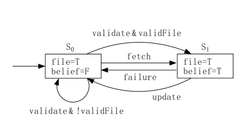
Figure 6: The transition system of the server

For the client, its initial states set are composed of $s_{0}$, $s_{1}$ and $s_{2}$. The state $s_{0}$ ($s_{1}$) represents that the client has no file copy in its cache and believes that the file is valid (invalid). The state $s_{2}$ describes that the client has a file copy and believes it is invalid. Therefore, if the client starts as state $s_{2}$, it will send the message $val$ to ask the server whether or not the file copy in its cache is valid; while if the client starts as state $s_{0}$ or $s_{1}$, it will send the message $fetch$ to get the valid file directly from the server. In addition, the state $s_{3}$ means that the client has a file copy and believes the file copy is valid. When the client receives the message $inval$ from the server, it will transfer from $s_{3}$ ($s_{2}$) to $s_{0}$ or $s_{1}$, which means that the server notifies the client that the copy is no longer valid and the client should discard the copy in its cache (as there is no file copy, so the validity of the file is unknown, i.e., the variable $belief$ equals either $true$ or $false$). When the client receives the message $failure$ from the system, it will transfer from $s_{3}$ to $s_{2}$, which means there is something wrong in the communications between the client and server and they should check again the coherence of the file. The transition system of a client is represented in Fig.7.

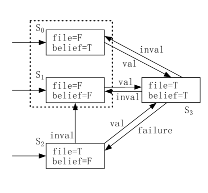
Figure 7: The transition system of the client

In this case study, the pair of states $\{s_{0},s_{1}\}$ of the client (indicated by dashed line in Fig.7) has a symmetric relation and this can be abstracted. This corresponds to the value of the variable $belief$ being irrelevant when the variable $file$ is $F$. Thus we can model the transition relation of the client by a 3-valued variable as shown in Fig.8. When this model is composed with the rest of the AFS2 model, we get a 3-valued model-checking problem which can not be directly verified using a classical model-checking algorithm.

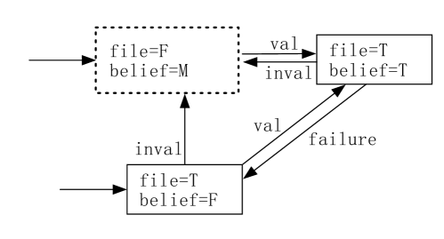
Figure 8: The abstracted transition system of the client

In addition, it might happen that the server sends an $inval$ message to some client that believes that its copy is valid. During the transmission, a property may hold since the client believes that its copy is valid while the server does not. Therefore, this transmission delay must be taken into account. We model the delay with the shared variable $time_{i}$.

The linear-time properties of AFS2 system we verified appeared as follows.

P1: If a client believes that a cached file is valid, then the server that is the authority on the file believes the client’s copy is valid.

This property can be represented by a linear-temporal logic formulae as follows.

For one client:

$\square(Client_{i}.belief\wedge Client_{i}.file\rightarrow(server.belief_{i}\wedge Server.file_{i})\vee\neg time_{i})\wedge(Server.out_{i}=val\rightarrow Server.belief_{i}\wedge Sever.file_{i})$.

For $N$ clients:

$\square(\bigwedge_{i=1}^{N}(Client_{i}.belief\wedge Client_{i}.file\rightarrow(server.belief_{i}\wedge Server.file_{i})\vee\neg time_{i})\wedge(Server.out_{i}=val\rightarrow Server.belief_{i}\wedge Sever.file_{i}))$.

P2: if a server believes that the client’s copy is valid, then the client believes the cached file on the client is valid.

This property can be written as a linear-temporal logic formulae as follows.

For one client:

$\square(Server.belief_{i}\wedge Server.file_{i}\rightarrow((Client_{i}.belief\wedge Client_{i}.file)\vee\neg time_{i})\wedge(Server.out_{i}=(validate\wedge valid-file)\vee fetch\rightarrow Server.belief_{i}\wedge Sever.file_{i})$.

For $N$ clients:

$\square(\bigwedge_{i=1}^{N}(Server.belief_{i}\wedge Server.file_{i}\rightarrow((Client_{i}.belief\wedge Client_{i}.file)\vee\neg time_{i})\wedge(Server.out_{i}=(validate\wedge valid-file)\vee fetch\rightarrow Server.belief_{i}\wedge Sever.file_{i}))$.

The results are summarized in Fig.9, Table 1 and Table 2. The property $P1$ is correct, while the property $P2$ is wrong and a counterexample is given. There are several linear-temporal logic symbolic model checking tools as explained in Ref.[44]. The tool NuSMV 2.5.4 running on Pentium (R) Dual-Core E5800 with 3.20GHz processor and 2.00GB RAM, under ubuntu-11.04-desktop-i386, is used for the verification in this case study.

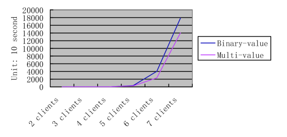
Figure 9: The running times of the multi-valued and classical model checking for AFS2

Table 1: The results of classical model checking for AFS2

	User Time	BDD Nodes	Transition Rules	States
2 Clients	0.184s	33667	$7^{2}$	(2$\times 4)^{2}$
3 Clients	15.917s	310383	$7^{3}$	(2$\times 4)^{3}$
4 Clients	20.845s	1299115	$7^{4}$	(2$\times 4)^{4}$
5 Clients	322.224s	235026	$7^{5}$	(2$\times 4)^{5}$
6 Clients	4054.901s	443001	$7^{6}$	(2$\times 4)^{6}$
7 Clients	17885.806s	1852283	$7^{7}$	(2$\times 4)^{7}$

Table 2: The results of multi-valued model checking for AFS2

	User Time	BDD Nodes	Transition Rules	States
2 Clients	0.1724s	33667	$5^{2}$	(2$\times 3)^{2}$
3 Clients	13.889s	1061221	$5^{3}$	(2$\times 3)^{3}$
4 Clients	15.521s	1360904	$5^{4}$	(2$\times 3)^{4}$
5 Clients	253.944s	223831	$5^{5}$	(2$\times 3)^{5}$
6 Clients	2353.939s	612687	$5^{6}$	(2$\times 3)^{6}$
7 Clients	14065.975s	1318587	$5^{7}$	(2$\times 3)^{7}$

In this case study, we use the classical model-checking algorithm two times to verify the model-checking problem of linear-time property in mv-logic. On the other hand, in classical model-checking of the original problem, the state space of the model is more complex than the abstracted model represented by mv-logic (as shown in Table 1 and Table 2). The overall time complexity of mv-logic is smaller than that in classical case as shown in Fig. 9, Table 1 and Table 2.

8 Conclusions

Multi-valued model checking is a multi-valued extension to classical model checking. Both the model of the system and the specification take values over a de Morgan algebra. Such an extension enhances the expressive power of temporal logic and allows reasoning under uncertainty. Some of the applications that can take advantage of the multi-valued model checking are abstract techniques, reasoning about conflicting viewpoints and temporal logic query checking. In this paper, we studied several important multi-valued linear-time properties and the multi-valued model checking corresponding to them. Concretely, we introduced the notions of safety, invariance, liveness, persistence and dual-persistence in the multi-valued logic system. Since the law of non-contradiction (i.e., $a\wedge\neg a=0$) and the law of excluded-middle (i.e., $a\vee\neg a=1$) do not hold in multi-valued logic, the linear-time properties introduced in this paper have new forms compared to those in classical logic. For example, the safety property in mv-logic is defined using good prefixes instead of bad prefixes. In which, model checking of the multi-valued invariant property and the persistence property can be reduced to their classical counterparts, the related algorithms were also presented. Furthermore, we introduced the notions of lattice-valued finite automata including Büchi and Rabin automata. With these notions, we gave the verification methods of multi-valued regular safety properties and multi-valued $\omega$-regular properties. Since the law of non-contradiction and the law of excluded middle do not hold in multi-valued logic, the verification methods gave here were direct and not a direct extension of the classical methods. This was in contrast to the classical verification methods. A new form of multi-valued model checking with membership degree (compared to that in [9]) was also introduced. The related verification algorithms were presented.

On the other hand, in literature there was much work on weighted model checking ([7], c.f.[16]) that used weighted automata as models of systems. Weighted model checking uses a semiring as weight structure of weighted automata. Since a De-Morgan algebra is a distributive lattice, and a distributive lattice is a semiring, weighted model checking with weights in a De-Morgan algebra is a special case of semiring-weighted model checking. This kind of weighted model checking seems to be closed related with multi-valued model checking. However, they are different. There are some essential differences between multi-valued model checking and weighted model checking. First, weighted model checking is still based on classical logic, i.e., two-valued logic, while mv-model checking is based on mv-logic. Then the uncertainty represented by the multi-valued logic systems can be considered sufficiently in multi-valued model checking. Second, there is few work on weighted LTL model checking, let alone the weighted model checking of the multi-valued safety property and liveness property, which formed the main topic of this paper. We should mention the recent paper [39], in which the description of the classical linear-time properties using possibility measures was given, but not any work on the uncertainty linear-time properties, which was the topic of this paper.

There was much work on the multi-valued model checking, for example, [5, 6, 8, 10, 12, 13, 9, 21, 28, 32, 16]. As we said in the introduction part, we adopted a direct method to model checking of multi-valued linear-time properties instead of those existing indirect methods. More precisely, the existing methods of mv-model checking still used the classical method with some minor correction. That is, instead of checking $TS\models P$ for an mv-linear time property $P$ using the inclusion of the trace function $Traces(TS)\subseteq P$, the existing method only checked the membership degree of the language $Traces(TS)\cap L({\cal A}_{\neg P})$, where ${\cal A}_{\neg P}$ is an mv-Büchi automaton such that $L({\cal A}_{\neg P})=\neg P$. However, as said in Ref. [2], the equivalences and preorders between transitions systems that “correspond” to linear temporal logic are based on trace inclusion and equality. In this paper, we adopted the multi-valued model checking of $TS\models P$ by using directly the inclusion relation $Traces(TS)\subseteq P$. In general, we used the implication connective as a primitive connective in mv-logic which satisfies $a\leq b$ iff $a\rightarrow b=1$ to define the membership degree of the inclusion of $Traces(TS)$ into $P$. We give further comments on the comparison of our method to the existing approaches as follows.

Since we chose $\rightarrow$ as a primitive connective in mv-logic, the classical logic could not be embedded into the mv-logic in a unique way as done in [13]. For example, $a\rightarrow b$ and $\neg a\vee b$ are equivalent in classical logic, but not in mv-logic. This is one of the main difference of our method to those existing approaches. Due to this difference, we verify that the system model $TS$ satisfies the specified linear-time property $P$, i.e., $TS\models P$ directly using the inclusion $Traces(TS)\subseteq P$ instead of $L({\cal A})\cap L({\cal A}_{\neg P})=\emptyset$, where ${\cal A}_{\neg P}$ is a multi-valued Büchi automaton such that $L({\cal A}_{\neg P})=\neg P$. Regarding expressiveness, we mainly studied the model-checking methods of linear-time properties in mv-logic systems. Compared with the work [9], we use more general lattices instead of finite total order lattices to represent the truth values in the mv-logic. All the properties studied in [9] can be tackled using our method, and another different view can be given. For the multi-valued model of CTL, etc, as done in [8, 12, 10, 13], our method could be also applied which forms one direction of future work.

Therefore, the approach proposed in this paper can be thought of as complementary to those mentioned methods of multi-valued model checking. The examples and case study show the validity and performance of the method proposed in this article. In the future work, we shall give some further comparison of our method with those available methods in multi-valued model checking and give some experiments. Another direction is to extend the method used in this paper to multi-valued LTL or CTL.

Appendix A The equivalent definition of multi-valued transition system

In an mv-TS, $TS=(S,Act,\rightarrow,I,AP,L)$, if the labeling function is $L:S\rightarrow l^{AP}$ or $L:S\times AP\rightarrow l$, then we have another form of mv-TS. The later is used in Ref. [10] (which is called mv-Kripke structure). There, $L(s,A)$ represents the truth-value of the atomic proposition $A$ at state $s$.

In this case, the trace function of $TS$ needs to be redefined as follows.

Since $TS$ is finite, we can assume that $Im(L)=\{d_{1},\cdots,d_{t}\}$. For any $d\in Im(L)$, define $L_{d}:S\rightarrow 2^{AP}$ as follows,

$L_{d}(s)=\{A\in AP|L(s,A)\geq d\}$.

Then $Traces(TS):(2^{AP})^{\omega}\rightarrow l$ is defined in the following manner. Let $A_{0}A_{1}\cdots\in(2^{AP})^{\omega}$, $\rho=s_{0}\alpha_{1}s_{1}\alpha_{2}\cdots$ a run of $TS$ with states sequence $\pi=s_{0}s_{1}\cdots$, such that $\eta(s_{i},\alpha_{i+1},s_{i+1})=r_{i+1}$ and $L_{d_{\phi(i)}}(s_{i})=A_{i}$ for any $i\geq 0$, where $d_{\phi(i)}$ is an element of $Im(L)$ with $\phi(i)\in\{1,\cdots,t\}$. Then,

$Traces(TS)(A_{0}A_{1}\cdots)=\bigvee\{r_{0}\wedge d_{\phi(0)}\wedge r_{1}\wedge d_{\phi(1)}\wedge\cdots|\rho=s_{0}\alpha_{1}s_{1}\alpha_{2}\cdots$ is a run of $TS$ with states sequence $\pi=s_{0}s_{1}\cdots$, such that $\eta(s_{i},\alpha_{i+1},s_{i+1})=r_{i+1}$ and $L_{d_{\phi(i)}}(s_{i})=A_{i}$ for any $i\geq 0\}$.

We construct a new mv-TS from $TS$ with ordinary labeling function which has the same traces function as the original mv-TS, $TS$.

Let $S^{\prime}=S\times\{1,\cdots,t\}$. The initial distribution $I^{\prime}:S^{\prime}\rightarrow l$ is defined by $I^{\prime}(s,i)=I(s)\wedge d_{i}$, $\rightarrow^{\prime}\subseteq S^{\prime}\times Act\times S^{\prime}\times l$ is defined by $\eta^{\prime}((s,i),\alpha,(s^{\prime},i^{\prime}))=d_{i}\wedge\eta(s,\alpha,s^{\prime})\wedge d_{i^{\prime}}$, and $L^{\prime}:S^{\prime}\rightarrow 2^{AP}$ is defined by $L^{\prime}(s,i)=L_{d_{i}}(s)=\{A\in AP|L(s,A)\geq d_{i}\}$. Then we have a new mv-TS, $TS^{\prime}=(S^{\prime},Act,\rightarrow^{\prime},I^{\prime},AP,L^{\prime})$. Let us calculate the traces function of $TS^{\prime}$ in the sequel.

For $A_{0}A_{1}\cdots\in(2^{AP})^{\omega}$,

$Traces(TS^{\prime})(A_{0}A_{1}\cdots)=\bigvee\{\bigwedge_{i\geq 0}r_{i}^{\prime}|$ there exists a run $\rho=s_{0}^{\prime}\alpha_{1}s_{1}^{\prime}\alpha_{2}\cdots$ with states sequence $\pi^{\prime}=s_{0}^{\prime}s_{1}^{\prime}\cdots$, such that $\eta(s_{i}^{\prime},\alpha_{i+1},s_{i+1}^{\prime})=r_{i+1}^{\prime}$ and $L^{\prime}(s_{i}^{\prime})=A_{i}$ for any $i\geq 0\}$.

For a run $\rho=s_{0}^{\prime}\alpha_{1}s_{1}^{\prime}\alpha_{2}\cdots$ in $TS^{\prime}$, let $s_{i}^{\prime}=(s_{i},\phi(i))$ and $d_{\phi(i)}\in Im(L)$. Then from the definition of $I^{\prime}$, $\rightarrow^{\prime}$, and $L^{\prime}$, we know that

$r_{0}^{\prime}=I^{\prime}(s_{0},\phi(0))=I(s_{0})\wedge d_{\phi(0)}=r_{0}\wedge d_{\phi(0)}$, where $r_{0}=I(s_{0})$.

$r_{i}^{\prime}=\eta^{\prime}((s_{i-1},\phi(i-1)),\alpha_{i},(s_{i},\phi(i)))=d_{\phi(i-1)}\wedge\eta(s_{i-1},\alpha_{i},s_{i})\wedge d_{\phi(i)}=d_{\phi(i-1)}\wedge r_{i}\wedge d_{\phi(i)}$ for $i\geq 1$.

Thus, $\bigwedge_{i\geq 0}r_{i}^{\prime}=r_{0}\wedge d_{\phi(0)}\wedge r_{1}\wedge d_{\phi(1)}\wedge\cdots$ and $A_{i}=L^{\prime}(s_{i}^{\prime})=L_{\phi(i)}(s_{i})$, which is the same as those in the definition of $Traces(TS)(A_{0}A_{1}\cdots)$.

Hence, $Traces(TS^{\prime})(A_{0}A_{1}\cdots)=Traces(TS)(A_{0}A_{1}\cdots)$ for any $A_{0}A_{1}\cdots\in(2^{AP})^{\omega}$. It follows that $Traces(TS^{\prime})=Traces(TS)$. Hence, $TS^{\prime}$ is equivalent to $TS$ in the sense of trace function. $\Box$

Appendix B The proof of Proposition 6

(1) is obvious.

(2) The inclusion $Closure(P_{1})\cup Closure(P_{2})\subseteq Closure(P_{1}\cup P_{2})$ is obvious. Conversely, let $X=Im(P_{1})\cup Im(P_{2})$, and let $l_{1}$ be the sublattice generated by $X$, then $l_{1}$ is a finite distributive lattice ([3, 35]). Observing that the three sets $Im(Closure(P_{1}))$, $Im(Closure(P_{2}))$ and $Im(Closure(P_{1}\cup P_{2}))$ are subsets of $l_{1}$, to show $Closure(P_{1}\cup P_{2})\subseteq Closure(P_{1})\cup Closure(P_{2})$, it suffices to show that, for any $m\in JI(l_{1})$ and $\sigma\in(2^{AP})^{\omega}$, $m\leq Closure(P_{1}\cup P_{2})(\sigma)$ implies that $m\leq Closure(P_{1})(\sigma)$ or $m\leq Closure(P_{2})(\sigma)$. By the definition of $Closure$ operator, $m\leq Closure(P_{1}\cup P_{2})(\sigma)$ implies that, for any $\theta\in Pref(\sigma)$, there exists $\tau\in(2^{AP})^{\omega}$ such that $m\leq P_{1}(\theta\tau)\vee P_{2}(\theta\tau)$, it follows that $m\leq P_{1}(\theta\tau)$ or $m\leq P_{2}(\theta\tau)$. Let $Pref_{1}=\{\theta\in Pref(\sigma)|m\leq P_{1}(\theta\tau)$ for some $\tau\in(2^{AP})^{\omega}\}$, and $Pref_{2}=\{\theta\in Pref(\sigma)|m\leq P_{2}(\theta\tau)$ for some $\tau\in(2^{AP})^{\omega}\}$. Then $Pref_{1}\cup Pref_{2}=Pref(\sigma)$. Since $Pref(\theta)$ is infinite as a set, it follows that $Pref_{1}$ or $Pref_{2}$ is infinite. Without loss of generality, let us assume that $Pref_{1}$ is infinite. Then, for any $\theta\in Pref(\sigma)$, since $Pref_{1}$ is infinite, there is $\theta_{1}\in Pref_{1}$ such that $\theta\in Pref(\theta_{1})$, and $m\leq P_{1}(\theta_{1}\tau_{1})$ for some $\tau_{1}\in(2^{AP})^{\omega}$. In this case, there exists $\tau\in(2^{AP})^{\omega}$ such that $\theta_{1}\tau_{1}=\theta\tau$ and $m\leq P_{1}(\theta_{1}\tau_{1})=P_{1}(\theta\tau)$. Hence, by the definition of $Closure(P_{1})$, it follows that $m\leq Closure(P_{1})(\sigma)$.

(3) By condition (1), we have $Closure(P)\subseteq Closure(Closure(P))$. Conversely, for any $\sigma\in(2^{AP})^{\omega}$, we have

$Closure(Closure(P))(\sigma)=\bigwedge\{\bigvee_{\tau\in(2^{AP})^{\omega}}Closure(P)(\theta\tau)|\theta\in Pref(\sigma)\}$.

On the other hand, for $Closure(P)(\theta\tau)$, since $\theta\in Pref(\theta\tau)$, we have

$Closure(P)(\theta\tau)=\bigwedge\{\bigvee_{\tau_{1}\in(2^{AP})^{\omega}}P(\theta_{1}\tau_{1})|\theta_{1}\in Pref(\theta\tau)\}\leq\bigvee_{\tau_{1}\in(2^{AP})^{\omega}}P(\theta\tau_{1})$.

Hence,we have

$Closure(Closure(P))(\sigma)=\bigwedge\{\bigvee_{\tau\in(2^{AP})^{\omega}}Closure(P)(\theta\tau)|\theta\in Pref(\sigma)\}\leq\bigwedge\{\bigvee_{\tau\in(2^{AP})^{\omega}}$ $\bigvee_{\tau_{1}\in(2^{AP})^{\omega}}P(\theta\tau_{1})|\theta\in Pref(\sigma)\}=\bigwedge\{\bigvee_{\tau_{1}\in(2^{AP})^{\omega}}P(\theta\tau_{1})|\theta\in Pref$ $(\sigma)\}=Closure(P)(\sigma)$.

This shows that $Closure(Closure(P))\subseteq Closure(P)$.

Therefore, $Closure(Closure(P))=Closure(P)$. $\Box$

(4) is obvious.

Appendix C The proof of Theorem 19

As a preliminary to show Theorem 19, we need a proposition to characterize mv-$\omega$-regular languages. The following results are contained in [15, 18], we include a proof for its completeness.

Proposition 22.

For an mv-$\omega$ language $f:\Sigma^{\omega}\rightarrow l$, the following statements are equivalent:

(1) $f$ is an mv-$\omega$-regular language, i.e., $f$ can be accepted by an $l$-VBA.

(2) $Im(f)$ is finite and $f_{a}$ is a $\omega$-regular language (which can be accepted by a Büchi automaton) over $\Sigma$ for any $a\in Im(f)$.

(3) There exist finite elements $m_{1},\cdots,m_{k}$ in $l$ and finite $\omega$-regular languages ${\cal L}_{1},\cdots,{\cal L}_{k}$ over $\Sigma$ such that

$f=\bigcup_{i=1}^{k}m_{i}\wedge{\cal L}_{i}$.

Proof:  (1)$\Longrightarrow$ (2): Assume that $f$ is accepted by an $l$-VBA, ${\cal A}=(Q,\Sigma,\delta,I,F)$. Let $X=Im(I)\cup Im(\delta)\cup Im(F)$. Since $Q$ and $\Sigma$ are finite as two sets, $X$ is finite as a subset of $l$. Let $l_{1}$ be the sublattice of $l$ generated by $X$, then $l_{1}$ is a finite distributive lattice ([3, 35]), and any element of $l_{1}$ can be represented as a finite join of join-irreducible elements of $l_{1}$. For any $m\in JI(l_{1})$, let ${\cal A}_{m}=(Q,\Sigma,\delta_{m},I_{m},F_{m})$. Then ${\cal A}_{m}$ is a classical Büchi automaton and thus $L_{\omega}({\cal A}_{m})$ is $\omega$-regular.

Let us show that $L_{\omega}({\cal A})_{m}=L_{\omega}({\cal A}_{m})$. This is because, for any $w=\sigma_{1}\sigma_{2}\cdots\in\Sigma^{\omega}$,

$w\in L_{\omega}({\cal A}_{m})$

iff

for any $i\geq 0$, there exists $q_{i}\in Q$ such that $q_{0}\in I_{m}$, $(q_{i},\sigma_{i+1},q_{i+1})\in\delta_{m}$, and $J=\{i|q_{i}\in F_{m}\}$ is an infinite subset of N;

iff

for any $i\geq 0$, there exists $q_{i}\in Q$ such that $I(q_{0})\geq m$, $\delta(q_{i},\sigma_{i+1},q_{i+1})\geq m$, and there exists an infinite subset $J$ of N such that $F(q_{j})\geq m$ for any $j\in J$;

iff

for any $i\geq 0$, there exists $q_{i}\in Q$ and infinite subset $J$ of N such that $I(q_{0})\geq m$ and $\bigwedge_{i\geq 0}\delta(q_{i},\sigma_{i+1},q_{i+1})\wedge\bigwedge_{j\in J}F(q_{j})\geq m$;

iff

$\bigvee\{I(q_{0})\wedge\bigwedge_{i\geq 0}\delta(q_{i},\sigma_{i+1},q_{i+1})\wedge\bigwedge_{j\in J}F(q_{j})|q_{i}\in Q$ for any $i\geq 0$ and $J$ is an infinite subset of N$\}\geq m$;

iff

$L_{\omega}({\cal A})(w)\geq m$

iff

$w\in L_{\omega}({\cal A})_{m}$.

Hence, $L_{\omega}({\cal A})_{m}$ is $\omega$-regular for any $m\in JI(l_{1})$.

Furthermore, for any $a\in Im(f)=Im(L_{\omega}({\cal A}))$, there exists finite join-irreducible elements $m_{1},\cdots,m_{k}$ in $l_{1}$ such that $a=\bigvee_{i=1}^{k}m_{i}$. Then

$f_{a}=\bigcap_{i=1}^{k}f_{m_{i}}$.

Since $f_{m_{i}}$ is $\omega$-regular and $\omega$-regular languages are closed under finite intersection, it follows that $f_{a}$ is $\omega$-regular.

$(2)\Longrightarrow$ (3) is obvious.

(3) $\Longrightarrow$ (1). Since ${\cal L}_{i}$ is $\omega$-regular, there exists a Büchi automaton ${\cal A}_{i}=(Q_{i},\Sigma,\delta_{i},I_{i},F_{i})$ such that $L_{\omega}({\cal A}_{i})={\cal L}_{i}$, for any $i=1,\cdots,k$. If we let $Q=\bigcup\{i\}\times Q_{i}$, and define $I,F:Q\rightarrow l$ and $\delta:Q\times\Sigma\times Q\rightarrow l$ as,

$${I(i,q)}=\left\{\begin{array}[]{ll}m_{i},&\textrm{if $q\in I_{i}$}\\ 0,&\textrm{otherwise,}\\ \end{array}\right.$$

$${F(i,q)}=\left\{\begin{array}[]{ll}m_{i},&\textrm{if $q\in F_{i}$}\\ 0,&\textrm{otherwise,}\\ \end{array}\right.$$

$${\delta((i,q),\sigma,(j,p))}=\left\{\begin{array}[]{ll}m_{i},&\textrm{if $i=j$ and $(q,\sigma,p)\in\delta_{i}$}\\ 0,&\textrm{otherwise,}\\ \end{array}\right.$$

for any $(i,q),(j,p)\in Q$. This constructs a new mv-$\omega$-Büchi automaton ${\cal A}=(Q,\Sigma,\delta,I,F)$. Let us show that $L_{\omega}({\cal A})=f$.

In fact, for any $w=\sigma_{1}\sigma_{2}\cdots\in\Sigma^{\omega}$, for any $i\geq 0$, if there exist $q_{i}^{\prime}\in Q$ and infinite subset $J$ of N such that $I(q_{0}^{\prime})\wedge\bigwedge_{i\geq 0}\delta(q_{i}^{\prime},\sigma_{i+1},q_{i+1}^{\prime})\wedge\bigwedge_{j\in J}F(q_{j}^{\prime})>0$. By definitions of $I,F$ and $\delta$, there exists $j_{i}$, $1\leq j_{i}\leq k$ and $q_{i}\in Q$ such that $q_{i}^{\prime}=(j_{i},q_{i})$ and $q_{0}\in I_{j_{i}}$, $(q_{i},\sigma_{i},q_{i+1})\in\delta_{j_{i}}$, and for any $j\in J$, $q_{j}\in F_{j_{i}}$. It follows that $w\in{\cal L}_{j_{i}}$. Hence, by the definition of $L_{\omega}({\cal A})$, we have

$L_{\omega}({\cal A})(w)=\bigvee\{m_{i}|w\in{\cal L}_{i}\}=f(w)$.

Hence, $f$ is mv-$\omega$-regular. $\Box$

Proposition 23.

Let $f_{1},\cdots,f_{k}$ ($k\geq 2$) be finite mv-$\omega$-languages from $\Sigma^{\omega}$ into $l$ which can be accepted by some $l$-VDRAs. Then their join $f_{1}\cup\cdots\cup f_{k}$ can also be accepted by an $l$-VDRA.

Proof:  For simplicity, we give the proof for the case $k=2$. The other case can be proved by induction on $k$.

Assume that $f_{i}$ can be recognized by an $l$-VDRA ${\cal A}_{i}=(Q_{i},\Sigma,\delta_{i},q_{i0},{\cal F}_{i})$ for $i=1,2$, respectively. Let us show that $f=f_{1}\cup f_{2}$ can also be accepted by some $l$-VDRA. We explicitly construct such $l$-VDRA, ${\cal A}=(Q,\Sigma,\delta,q_{0},{\cal F})$, as follows, where $Q=Q_{1}\times Q_{2}$, $\delta=\delta_{1}\times\delta_{2}$ (that is, $\delta((q_{1},q_{2}),\sigma)=(\delta(q_{1},\sigma),\delta(q_{2},\sigma))$), $q_{0}=(q_{10},q_{20})$, and ${\cal F}:2^{Q_{1}\times Q_{2}}\times 2^{Q_{1}\times Q_{2}}\rightarrow l$ is defined by,

$${{\cal F}((H,K))}=\left\{\begin{array}[]{ll}{\cal F}_{1}((H_{1},K_{1})),&\textrm{if $H=H_{1}\times Q_{2}$ and $K=K_{1}\times Q_{2}$}\\ {\cal F}_{2}((H_{2},K_{2})),&\textrm{if $H=Q_{1}\times H_{2}$ and $K=Q_{1}\times K_{2}$}\\ {\cal F}_{1}((H_{1},K_{1}))\vee{\cal F}_{2}((H_{2},K_{2})),&\textrm{if $H=H_{1}\times Q_{2}\cup Q_{1}\times H_{2}$ and}\\ &\textrm{$K=K_{1}\times K_{2}$}\\ 0,&\textrm{otherwise,}\\ \end{array}\right.$$

By the definition of $L_{\omega}({\cal A})$, $L_{\omega}({\cal A}_{1})$ and $L_{\omega}({\cal A}_{2})$, it is obvious that $L_{\omega}({\cal A}_{1})\cup L_{\omega}({\cal A}_{2})\subseteq L_{\omega}({\cal A})$.

Conversely, let $X=Im({\cal F}_{1})\cup Im({\cal F}_{1})$ and $l_{1}$ be the sublattice generated by $X$, then $l_{1}$ is a finite distributive lattice. The inclusion $Im({\cal F})\subseteq l_{1}$ is obvious and thus $Im(L_{\omega}({\cal A}))\subseteq l_{1}$. To show $L_{\omega}({\cal A})\subseteq L_{\omega}({\cal A}_{1})\cup L_{\omega}({\cal A}_{2})$, it suffices to show that, for any $\sigma\in\Sigma^{\omega}$ and for any $m\in JI(l_{1})$, if $m\leq L_{\omega}({\cal A})(\sigma)$, then $m\leq L_{\omega}({\cal A}_{1})(\sigma)$ or $m\leq L_{\omega}({\cal A}_{2})(\sigma)$. By the definition of $L_{\omega}({\cal A})(\sigma)$, if $m\leq L_{\omega}({\cal A})(\sigma)$, then there exists $(H,K)\in 2^{Q}\times 2^{Q}$ such that $m\leq{\cal F}((H,K))$, and if we let $q_{i+1}=(q_{1,i+1},q_{2,i+1})=\delta(q_{i},\sigma)=(\delta_{1}(q_{1i},\sigma),\delta_{2}(q_{2i},\sigma))$ for $i=0,1,\cdots$, such that $(\exists n\geq 0.\forall m\geq n.q_{m}\not\in H)\wedge(\forall n\geq 0.\exists m\geq n.q_{m}\in K)$. By the definition of ${\cal F}$, we have three cases to consider:

Case 1: $H=H_{1}\times Q_{2}$, $K=K_{1}\times Q_{2}$. In this case, we have $m\leq{\cal F}((H,K))={\cal F}((H_{1},K_{1}))$. Then the sequence $q_{0}q_{1}\cdots$ satisfies the condition $(\exists n\geq 0.\forall m\geq n.q_{m}=(q_{1m},q_{2m})\not\in H_{1}\times Q_{2})\wedge(\forall n\geq 0.\exists m\geq n.q_{m}=(q_{1m},q_{2m})\in K_{1}\times Q_{2})$. The later condition implies that $(\exists n\geq 0.\forall m\geq n.q_{1m}\not\in H_{1})\wedge(\forall n\geq 0.\exists m\geq n.q_{1m}\in K_{1})$. By the definition of $L_{\omega}({\cal A}_{1})(\sigma)$, it follows that ${\cal F}_{1}((H_{1},K_{1}))\leq L_{\omega}({\cal A}_{1})(\sigma)$. Hence, $m\leq L_{\omega}({\cal A}_{1})(\sigma)$.

Case 2: $H=Q_{1}\times H_{2}$, $K=Q_{1}\times K_{2}$. Similar to Case 1, we can prove that $m\leq L_{\omega}({\cal A}_{2})(\sigma)$.

Case 3: $H=H_{1}\times Q_{2}\cup Q_{1}\times H_{2}$ and $K=K_{1}\times K_{2}$. In this case, we have $m\leq{\cal F}((H,K))={\cal F}((H_{1},K_{1}))\vee{\cal F}((H_{2},K_{2}))$. Since $m\in JI(l_{1})$, it follows that $m\leq{\cal F}((H_{1},K_{1}))$ or $m\leq{\cal F}((H_{2},K_{2}))$. Consider the sequence $q_{0}q_{1}\cdots$, it satisfies the condition $(\exists n\geq 0.\forall m\geq n.q_{m}=(q_{1m},q_{2m})\not\in H_{1}\times Q_{2}\cup Q_{1}\times H_{2})\wedge(\forall n\geq 0.\exists m\geq n.q_{m}=(q_{1m},q_{2m})\in K_{1}\times K_{2})$. The later condition implies that $(\exists n\geq 0.\forall m\geq n.q_{1m}\not\in H_{1})\wedge(\forall n\geq 0.\exists m\geq n.q_{1m}\in K_{1})\wedge(\exists n\geq 0.\forall m\geq n.q_{1m}\not\in H_{2})\wedge(\forall n\geq 0.\exists m\geq n.q_{1m}\in K_{2})$. It follows that ${\cal F}_{1}((H_{1},K_{1}))\leq L_{\omega}({\cal A}_{1})(\sigma)$ and ${\cal F}_{2}((H_{2},K_{2}))\leq L_{\omega}({\cal A}_{2})(\sigma)$. Hence, $m\leq L_{\omega}({\cal A}_{1})(\sigma)$ or $m\leq L_{\omega}({\cal A}_{2})(\sigma)$.

This concludes that $L_{\omega}({\cal A})=L_{\omega}({\cal A}_{1})\cup L_{\omega}({\cal A}_{2})$. $\Box$

The proof of Theorem 19:

Let $f:\Sigma^{\omega}\rightarrow l$ be an mv-language accepted by an $l$-VDRA ${\cal A}=(Q,\Sigma,\delta,q_{0},{\cal F})$. By the definition of $L_{\omega}({\cal A})$, it follows that $Im(f)=Im(L_{\omega}({\cal A}))\subseteq Im({\cal F})$ and thus $Im(f)=Im(L_{\omega}({\cal A}))$ is a finite subset of $l$. For any $a\in Im(f)$, $f_{a}$ is obvious accepted by the classical Rabin automaton ${\cal A}_{a}=(Q,\Sigma,\delta,q_{0},{\cal F}_{a})$, and thus $f=L_{\omega}({\cal A})$ is a $\omega$-regular language. Hence, condition (2) in Proposition 22 holds for $f$, $f$ can be accepted by an $l$-VBA.

Conversely, if $f$ can be accepted by an $l$-VBA, then, by Proposition 22(3), there are finite elements $m_{1},\cdots,m_{k}$ in $l$ and finite $\omega$-regular languages ${\cal L}_{1},\cdots,{\cal L}_{k}$ over $\Sigma$ such that

$f=\bigcup_{i=1}^{k}m_{i}\wedge{\cal L}_{i}$.

For any $i$, since ${\cal L}_{i}$ is $\omega$-regular, there exists a deterministic Rabin automaton ${\cal A}=(Q,\Sigma,\delta,q_{0}$, $ACC)$ accepting ${\cal L}_{i}$, i.e., $L_{\omega}({\cal A})={\cal L}_{i}$. Construct an $l$-VDRA ${\cal A}^{\prime}$ from ${\cal A}$ as, ${\cal A}^{\prime}=(Q,\Sigma,\delta,q_{0},{\cal F})$, where ${\cal F}:2^{Q}\times 2^{Q}\rightarrow l$ is,

$${{\cal F}((H,K))}=\left\{\begin{array}[]{ll}m_{i},&\textrm{if $(H,K)\in ACC$}\\ 0,&\textrm{otherwise.}\\ \end{array}\right.$$

By a simple calculation, we have $L({\cal A}^{\prime})=m_{i}\wedge{\cal L}_{i}$. This shows that $m_{i}\wedge{\cal L}_{i}$ can be accepted by an $l$-VDRA for any $i$. By Proposition 23, and the equality $f=\bigcup_{i=1}^{k}m_{i}\wedge{\cal L}_{i}$, it follows that $f$ can be accepted by an $l$-VDRA. $\Box$

References

References

• [1] B. Alpern, F. Schneider, Defining liveness, Information Processing Letters, 21(1985) 181-185.
• [2] C. Baier, J. P. Katoen, Principles of Model Checking, MIT Press, Cambridge, Massacasetts, 2008.
• [3] G. Birkhoff, Lattice Theory, Third Edition, Amer. Math. Soc., Providence, Rhode Island, USA, 1973.
• [4] L. Bloc, P. Borowik, Multi-Valued Logics, Springer-Verlag, Berlin, 1992.
• [5] G. Bruns, P. Godefroid, Model checking partial state spaces with 3-valued temporal logics. In Proceedings of the 11th International Conference on Computer-Aided Verification (CAV 99), (Trento, Italy). Lecture Notes in Computer Science, vol. 1633, Springer, 1999, pp. 274-287.
• [6] G. Bruns, P. Godefroid, Generalized model checking: Reasoning about partial state spaces. In Proceedings of the 11th International Conference on Concurrency Theory (CONCUR 00), C.Palamidessi, eds., Lecture Notes in Computer Science, vol. 1877, Springer, 2000, pp. 168-182.
• [7] P. Buchholz, P. Kemper, Model checking for a class of weighted automata, CoRRcs.L0/0304021(2003).
• [8] M. Chechik, On interpreting results of model-checking with abstraction, CSRG Technical Report 417, University of Toronto, Department of Computer Science, September 2000.
• [9] M. Chechik, B. Deverux, A. Gurfinkel, Model-checking infinite state-space systems with fine-grained abstractions using SPIN. In Proceedings of the 8th SPIN Workshop on Model Checking Software, Toronto, Canada. Lecture Notes in Computer Science, vol. 2057, Springer, 2001, pp. 16-36.
• [10] M. Chechik, B. Devereux, A. Gurfinkel, S. Easterbrook, Multi-valued symbolic model-checking, ACM Transactions on Software Engineering and Methodology, 12(4)(2003) 371-408.
• [11] M. Ciric, M. Droste, J. Ignjatovic, H. Vogler, Determinization of weighted finite automata over strong bimonoids, Information Sciences, 180(18)(2010), 3497-3520.
• [12] M. Chechik, S. Easterbrook, V. Petrovykh, Model-checking over multi-valued logics, in: Proceedings of Formal Methods Europe (FME 01), Lecture Notes in Computer Science, Vol. 2021, Springer Verlag, Berlin, 2001, pp. 72-98.
• [13] M. Chechik, A. Gurfinkel, B. Devereux, A. Lai, S. Easterbrook, Data structures for symbolic multi-valued model-checking, Formal Methods in System Design, 29(2006) 295-344.
• [14] S. Demri, D. D Souza, An automata-theoretic approach to constraint LTL, Information and Computation, 205(3)(2007) 380-415.
• [15] M. Droste, W. Kuich, G. Rahonis, Multi valued MSO logics over words and trees, Fundamenta Informaticae, 84 (2008) 305-327.
• [16] M. Droste, W. Kuich, H. Vogler(Eds.), Handbook of Weighted Automata, Series: Monographs in Theoretical Computer Science. An EATCS Series, Springer-Verlag, Berlin-Heidelberg, 2009.
• [17] M. Droste, I.Meinecke, Weighted automata and weighted MSO logics for average and long-time behaviors, Information and Computation, 220-221(2012) 44-59.
• [18] M. Droste, H. Vogler, Weighted automata and multi-valued logics over arbitrary bounded lattices, Theoretical Computer Science, 418 (2012) 14-36.
• [19] S. Eilenberg, Automata, Languages and Machines, vol. A, vol B, Academic Press, New York, 1974.
• [20] M. Fitting, Many-valued modal logics, Fundamenta Informaticae, 15(3-4)(1991) 335-350.
• [21] P. Godefroid, R. Jagadeesan, On the expressiveness of 3-valuedmodels. In Proceedings of the 4th International Conference on Verification, Model Checking, and Abstract Interpretation (VMCAI 03), Lecture Notes in Computer Science, vol. 2575, Springer, 2003, pp. 206-222.
• [22] G. Grätzer, General Lattice Theory, 2nd ed., Birkhäuser-Verlag, Basel, 2003.
• [23] P. Hájek, Metamathematics of Fuzzy Logic, Kluwer Academic Publisher, Dordrecht, 1998.
• [24] S. Hazelhurst, Compositional Model Checking of Partially Ordered State Spaces. PhD thesis, Department of Computer Science, University of British Columbia, 1996.
• [25] G. Holzmann. The model checker SPIN, IEEE Transactions on Software Engineering, 23(5)(1997) 279-295.
• [26] J. E. Hopcroft , J. D. Ullman, Introduction to Automata Theory, Languages and Computation, Addison-Wesley, New York, 1979.
• [27] J.H. Howard, M.L. Kazar, S.G. Nochols, D.A. Nochols, M. Satyanarayanan, R.N. Sidebotham, M.J., West, Scale and performance in a distributed file system, ACM Transactions on Computer Systems, 6(1)(1988) 51-81.
• [28] M. Huth, R. Jagadeesan, D. A. Schmidt, Modal transition systems: a foundation for three-valued program analysis. In Proceedings of the 10th European Symposiumon Programming (ESOP 01), Lecture Notes in Computer Science, vol. 2028, Springer, 2001, pp. 155-169.
• [29] B. Khoussainov, A. Nerode, Automata Theory and its Applications, Birkäuser, Boston, 2001.
• [30] W. Kuich, G. Rahonis, Fuzzy regular languages over finite and infinite words, Fuzzy Sets and Systems, 157(2006) 1532-1549.
• [31] W.Kuich, A.Salomaa, Semirings, Automata, Languages, EATCS Monographs on Theoretical Computer Science, vol.5, Springer-Verlag, Berlin/Heidelberg/New York/Tokyo, 1986.
• [32] O. Kupferman, Y. Lustig, Lattice automata, Proceedings of VWCAI2007, Lecture Notes in Computer Science, vol. 4349, Springer, 2007, pp. 199-213.
• [33] O. Kupferman, M. Y. Vardi, Model checking of safety properties, Formal Methods in System Design, 19(2001) 291-314.
• [34] L. Lamport, Proving the correctness of multiprocess programs, IEEE Transactions on Software Engineering, 3(1977), 125-143.
• [35] Y. M. Li, Z. H. Li, Free semilattices and strongly free semilattices generated by partially ordered sets, Northeastern Mathematical Journal, 9(3)(1993) 359-366.
• [36] Y. M. Li, W. Pedrycz, Fuzzy finite automata and fuzzy regular expressions with membership values in lattice-ordered monoids, Fuzzy Sets and Systems, 156(2005) 68-92.
• [37] Y. M. Li, W. Pedrycz, Minimization of lattice finite automata and its application to the decomposition of lattice languages, Fuzzy Sets and Systems, 158(2007) 1423-1436.
• [38] Y. M. Li, Finite automata theory with membership values in lattices, Information Sciences, 181(2011) 1003-1017.
• [39] Y.M. Li, L.J. Li, Model checking of linear-time properties based on possibility measure, IEEE Transactions on Fuzzy Systems, 21(2013)(5) 842-854.
• [40] Y. Li, Z. Ma, Quantitative computation tree logic model checking based on generalized possibility measures, IEEE Transactions on Fuzzy Systems, 23(6)(2015) 2034-2047.
• [41] Y. Li, Quantitative model checking of linear-time properties based on generalized possibility measures, http://arxiv.org/abs/1601.06504.
• [42] Z. Manna, A. Pnueli, The Temporal Logic of Reactive and Concurrent Systems: Safety, Springer, Berlin, 1995.
• [43] K. McMillan, Symbolic Model Checking, Kluwer, Academic, 1993.
• [44] K.Y. Rozier, Linear temporal logic symbolic model checking, Computer Science Review, 5(2)(2011) 163-203.
• [45] S. Shoham, O. Grumberg, Compositional verification and 3-valued abstractions join forces, Information and Computation, 208(2)(2010) 178-202.
• [46] M. Y. Vardi, P. Wolper, Reasoning about infinite computations, Information and Computation, 115(1994) 1-37.