A Scale-Space Theory for Text

Abstract

Scale-space theory has been established primarily by the computer vision and signal processing communities as a well-founded and promising framework for multi-scale processing of signals (e.g., images). By embedding an original signal into a family of gradually coarsen signals parameterized with a continuous scale parameter, it provides a formal framework to capture the structure of a signal at different scales in a consistent way. In this paper, we present a scale space theory for text by integrating semantic and spatial filters, and demonstrate how natural language documents can be understood, processed and analyzed at multiple resolutions, and how this scale-space representation can be used to facilitate a variety of NLP and text analysis tasks.

1 Introduction

Physical objects in the world appear differently depending on the scale of observation/measurement. Take the tree as an example, meaningful observations range from molecules at the scale of nanometers, to leaves at centimeters, to branches at meters, and to forest at kilometers. This inherent property is ubiquitous and holds equally true for natural language. On the one hand, concepts are meaningful only at the right resolution, for instance, named entities usually range from unigram (e.g., “new”) to bigram (e.g., “New York”), to multigram (e.g., “New York Times”), and even to a whole long sequence (e.g., a song name “ Another Lonely Night In New York”). On the other hand, our understanding of natural language depends critically on the scale at which it is examined, for example, depending on how much detailed we would like to get into a document, our knowledge could range from a collection of “keywords”, to a sentence sketch named “title”, to a paragraph summary named “abstract”, to a page long “introduction” and finally to the entire content. The notion of scale is fundamental to the understanding of natural language, yet it was largely ignored by existing models for text representation, which include simple bag-of-word (BOW) or unigram language model (LM), n-gram or higher order LMs, and other more advanced text/language models [Iyer and Ostendorf, 1996, Manning and Schuetze, 1999, Metzler and Croft, 2005]. One key problem with many of these models is their inflexibility — they capture the semantic structure rather rigidly at only a single resolution (e.g., $n$-gram with a single fixed value of $n$). However, which scale is appropriate for a specific task is usually unknown a priori and in many cases even not homogeneous (e.g., a document may contain named entities of different length), making it impossible to capture the right meanings with a fixed single scale.

Scale space theory is a well-established and promising framework for multi-resolution representation, developed primarily by the computer vision and signal processing communities with complimentary motivations from physics and bio-vision. The key idea is to embed a signal into the scale space, i.e., to represent it as a family of progressively smoothed signals parameterized by a continuous variable of scale, where fine-resolution detailed structures are progressively suppressed by the convolution of the original signal with a smoothing kernel (i.e., a low pass filter with certain properties) [Witkin, 1983, Lindeberg, 1994].

In this paper, we adapt the scale-space model from image to text signals, proposing a novel framework that enables multi-resolution representation for documents. The adaptation poses substantial challenges as the structure of the semantic domain is nontrivially complicated than the spatial domains in traditional image scale space. We show how this can be made possible with a set of assumptions and simplifications. The scale-space model for text not only provides new perspectives for how text analysis tasks can be formulated and addressed, but also enables well-established computer vision tools to be adapted and applied to text processing, e.g., matching, segmentation, description, interests points detection, and classification. To stimulate further investigation in this promising direction, we initiate a couple of instantiations to demonstrate how this model can be used in a variety of NLP and text analysis tasks to make things easier, better, and most importantly, scale-invariant.

2 Scale Space Representation

The notion of scale space is applicable to signals of arbitrary dimensions. Let us consider the most common case, where it is applied to 2-dimensional signals such as images. Given an image $f(x_{1},x_{2})$, its scale-space representation $\gamma(x_{1},x_{2},s)$ is defined by:

$$\gamma(x_{1},x_{2},s)=f(x_{1},x_{2})*\ell(x_{1},x_{2},s)$$ (1)

$$= \int_{\mathbb{R}^{2}}f(x_{1}-u_{1},x_{2}-u_{2})\ell(u_{1},u_{2},s)du_{1}du_{2},$$

where $*$ denotes the convolution operator, and $\ell:\mathbb{R}^{2}\times\mathbb{R}_{+}\rightarrow\mathbb{R}$ is a smoothing kernel (i.e., a low pass filter) with a set of desired properties (i.e., the scale-space axioms [Lindeberg, 1994]). The bandwidth parameter $s$ is referred to as scale parameter since as $s$ increases, the derived image will become gradually smoother (i.e., blurred) and consequently more and more fine-scale structures will be suppressed.

It has been shown that the Gaussian kernel is the unique option that satisfies the conditions for linear scale space:

$$\ell(\textbf{x},s)=\frac{1}{\sqrt{2\pi s}}e^{-{(x_{1}^{2}+x_{2}^{2})}/{2s}}.\vspace{-5pt}$$ (2)

The resultant linear scale space representation $\gamma(x_{1},x_{2},s)$ can be obtained equivalently as a solution to the diffusion (heat) equation

$$\partial_{s}\gamma=\frac{1}{2}\triangle\gamma\vspace{-4pt}$$ (3)

with initial condition $\gamma(\textbf{x},0)=f(\textbf{x})$, where $\triangle$ denotes the Laplace operator which in a 2-dimensional spatial space corresponds to $\frac{\partial^{2}}{\partial x_{1}^{2}}+\frac{\partial^{2}}{\partial x_{2}^{2}}$. If we view $\gamma$ as a heat distribution, the equation essentially describes how it diffuses from initial value, $f$, in a homogeneous media with uniform conductivity over time $s$. As we can imagine, the distribution will gradually approach uniform and consequently the fine-scale structure of $f$ will be lost.

Scale-space theory provides a formal framework for handling the multi-scale nature of both the physical world and the human perception. Since its introduction in 1980s, it has become the foundation of many computer vision techniques and been widely applied to a large variety of vision/image processing tasks. In this paper, we show how this powerful tool can be adapted and applied to natural language texts.

3 Scale Space Model for Text

3.1 Word-level 2D Image Analogy of Text

A straightforward step towards textual sale space would be to represent texts in the way as image signal. In this section, we show how this can be made possible. Other alternative signal formulations will be discussed in the followed section.

Let $\mathcal{V}=\{v_{1},v_{2},\ldots,v_{M}\}$ be our vocabulary consisting of $M$ words, given a document $d$ comprised of a finite $N$-word sequence $d=w_{1}w_{2}\ldots w_{N}$, without any information loss, we can characterize $d$ as a 2D $N\times M$ binary matrix $f$, with the $(x,y)$-th entry $f(x,y)$ indicates whether or not the $y$-th vocabulary word $v_{y}$ is observed at the $x$-th position, i.e.: $f(x,y)=\delta(w_{x},v_{y})$, where $\delta(a,b)=1$ if $a=b$ and 0 otherwise. Hereafter, we will refer to the $x$-axis as spatial domain (i.e., positions in the document, $x\in\mathcal{X}=\{1,\ldots,N\}$), and $y$-axis as the semantic axis (i.e., indices in the vocabulary, $y\in\mathcal{Y}=\mathcal{V}$). This representation provides an image analogy to text, i.e., a document $f$ is equivalent to a black-and-white image except that here we have one spatial and one semantic domains, $(x,y)$, instead of two spatial domains, $(x_{1},x_{2})$.

Interestingly, scale-space representation can also be motivated by this binary model from a slightly different perspective, as a way of robust density estimation. We have the following definition:

Definition 1. A 2D text model $f\in\mathbb{R}_{+}^{N\times M}$ is a probabilistic distribution over the joint spatial-semantic space: $\mathcal{X}\times\mathcal{Y}\rightarrow\mathbb{R}_{+}$, $0\leqslant f(x,y)\leqslant 1$, $\int_{x}\int_{y}f(x,y)dxdy=1$.

This 2D text model defines the probability of observing a semantic word $y$ at a spatial position $x$. The binary matrix representation (after normalization) can be understood as an estimation of $f$ with kernel density estimators:

$$\vspace{-7pt}\textbf{f}(x,\cdot) =\frac{1}{N}\sum\nolimits_{i=1}^{N}\delta(w_{x}-w_{i})\textbf{e}_{x}^{\top},$$ (4)

$$\textbf{f}(\cdot,y) =\frac{1}{M}\sum\nolimits_{j=1}^{M}\delta(v_{y}-v_{j})\textbf{e}_{y},\vspace{-6pt}$$ (5)

where $\textbf{e}_{i}$ is the $i$-th column vector of an identity matrix, $\textbf{f}(x,\cdot)$ denotes the $x$-th row vector and $\textbf{f}(\cdot,y)$ the $y$-th column vector. Note that here the Dirac impulse kernels $\delta$ is used, i.e., words are unrelated either spatially or semantically. This contradicts the common knowledge since neighboring words in text are highly correlated both semantically [Mei et al., 2008] and spatially [Lebanon et al., 2007]. For instance, observing the word “New” indicates a high likelihood of seeing the other word “York” at the next position. As a result, it motivates more reliable estimate of $f$ by using smooth kernels such as Gaussian [Witkin, 1983, Lindeberg, 1994], which, as we will see, leads exactly to the Gaussian filtering used in the linear scale-space theory.

3.2 Textual Signals

The 2D binary matrix described above is not the only option we can work with in scale space. Generally speaking, any vector, matrix or even tensor representation of a document can be used as a signal upon which scale space filtering can be applied. In particular, we use the following in the current paper:

Word-level 2D signal, $f(x,y)$, is the binary matrix we described in §3.1. It records the spatial position for each word, and is defined on the joint spatial-semantic domains.

Bag-of-word 1D signal is the BOW representation $f(y)=\sum_{x}f(x,y)$, i.e., the 2D matrix is collapsed to a 1D vector. Since the spatial axis is wiped out, this signal is defined on the semantic domain alone.

Sentence-level 2D signal is a compromise between word-level 2D and the BOW signals. Instead of collapsing the spatial dimension for the whole document, we do it for each sentence. As a result, this signal, $f(x,y)$, records the position of each sentence; for a fixed position $x_{0}$, $f(x=x_{0},y)$ records the BOW of the corresponding sentence.

Topic 1D signal, $\textbf{f}(x)$, is composed of the topic embedding of each sentence and defined on the spatial domain only. Assume we have trained a topic model (e.g., Latent Dirichlet Allocation) on a universal corpus in advance, this signal is obtained by applying topic inference to each sentence and recording the topic embedding $\theta$${}_{x}\in\mathbb{R}^{k}$, where $k\ll M$ is the dimensionality of the topic space. Topic embedding is beneficial since it endows us the ability to address synonyms and polysemy. Also note that the semantic correlation may have been eliminated and consequently semantic smoothing is no longer necessary. In other words, although $\textbf{f}(x)$ is a matrix, we would rather treat it as a vector-variate 1D signal. All these textual signals involve either a semantic domain or both semantic and spatial domains. In the following, we investigate how scale-space filtering can be applied to these domains respectively.

3.3 Spatial Filtering

Spatial filtering has long been popularized in signal processing [Witkin, 1983, Lindeberg, 1994], and was recently explored in NLP by [Lebanon et al., 2007, Yang and Zha, 2010]. It can be achieved by convolution of the signal with a low-pass spatial filter, i.e., $\gamma(x,s)=f(x)*\ell(x,s)$. For texts, this amounts to borrowing the occurrence of words at one position from its neighboring positions, similar to what was done by a cache-based language model [Jelinek et al., 1991, Beeferman et al., 1999].

In order not to introduce spurious information, the filter $\ell$ need to satisfy a set of scale-space axioms [Lindeberg, 1994]. If we view the positions in a text as a spatial domain, the Gaussian kernel $\ell(x,s)=\frac{1}{\sqrt{2\pi s}}\exp(-x^{2}/2s)$ or its discrete counterpart

$$\ell(n,s)=e^{-s}I_{n}(s)$$ (6)

are singled out as the unique options that satisfy the set of axioms leading to the linear scale space, where $I_{n}(t)$ denotes the modified Bessel functions of integer order. Alternatively, if we view the position $x$ as a time variable as in the Markov language models, a Poisson kernel $\ell(n,s)=e^{-s}{s^{n}}/{n!}$ is more appropriate as it retains temporal causality (i.e., inaccessibility of future data).

3.4 Semantic Filtering

Semantic filtering attempts to smooth the probabilities of seeing words that are semantically correlated. In contrast to the spatial domain, the semantic domain has some unique properties. The first thing we notice is that, as semantic coordinates are nothing but indices to the dictionary, we can permute them without changing the semantic meaning of the representation. We refer to this property as permutation invariance. Semantic smoothing has been extensively explored in natural language processing [Manning and Schuetze, 1999, Zhai and Lafferty, 2004]. Classical smoothing methods, e.g., Laplacian and Dirichlet smoother, usually shrink the original distributions to a predefined reference distribution. Recent advances explored local smoothing where correlated words are smoothed according to their interrelations defined by a semantic network [Mei et al., 2008].

Given a semantic graph $\mathcal{G}_{v}$, where two correlated words $v_{y}$ and $v_{z}$ are connected with weight $\mu_{yz}$, semantic smoothing can be formulated as solving a graph-based optimization problem:

$$\begin{split}\min_{\gamma}&\quad(1-\lambda)\sum\nolimits_{y=1}^{M}\mu_{y}(\gamma_{y}-f_{y})^{2}\\ &+\lambda\sum\nolimits_{y=1}^{M}\sum\nolimits_{z=1}^{M}\mu_{yz}(\gamma_{y}-\gamma_{z})^{2},\\ \end{split}$$ (7)

where $0\leqslant\lambda\leqslant 1$ defines the tradeoff, $\mu_{y}$ weights the importance of the node $v_{y}$. Interestingly, the solution to Eqn.(7) is simply the convolution of the original signal with a specific kernel, i.e., $\gamma=f*\ell$.

Compared with spatial filtering, semantic filtering is, however, more challenging. In particular, the semantic domain is heterogeneous and not shift-invariant — the degree of correlation $\mu_{yz}$ depends on both coordinates $y$ and $z$ rather than their difference $(y-z)$. As a result, kernels that provably satisfy scale-space axioms are no longer feasible. To this end, we simply set aside these requirements and define kernels in terms of the dissimilarity $d_{yz}$ between a pair of words $y$ and $z$ rather than their direct difference $(y-z)$, that is, $\ell_{y}(y,z;s)=\ell_{x}(d_{yz},s)$, where we use $\ell_{y}$ to denote semantic kernel to distinguish from spatial kernels $\ell_{x}$. For Gaussian, this means $\ell_{y}(y,z;s)=\frac{1}{\sqrt{2\pi s}}\exp(-d_{yz}^{2}/2s)$.

3.5 Text Scale Space

Scale is vital for the understanding of natural language, yet it is nontrivial to determine which scale is appropriate for a specific task at hand in advance. As a matter of fact, the best choice usually varies from task to task and from document to document. Even within one document, it could be heterogeneous, varying from paragraph to paragraph and sentence to sentence. For the purpose of automatic modeling, there is no way to decide a priori which scale fits the best. More importantly, it might be impossible to capture all the right meanings at a single scale. Therefore, the only reasonable way is to simultaneously represent the document at multiple scales, which is exactly the notion of scale space.

Scale space representation embeds a textual signal into a continuous scale-space, i.e., by a family of progressively smoothed signals parameterized by continuous scale parameters. In particular, for a 2D textual signal $f(x,y)$, we have:

$$\gamma(x,y;s_{x},s_{y})=f(x,y)*\ell(x,y;s_{x},s_{y}),$$ (8)

where the 2D smoothing kernel $\ell$ is separable between spatial and semantic domains, i.e.,

$$\ell(x,y;s_{x},s_{y})=\ell_{x}(x,s_{x})\ell_{y}(y,s_{y}).$$ (9)

Note that we have two continuous scale parameters, the spatial scale $s_{x}\in\mathbb{R}_{+}$ and the semantic scale $s_{y}\in\mathbb{R}_{+}$. The case for 1D signals are even simpler as they only involve one type of kernels (spatial or semantic). For a 1D spatial signal $f(x)$, we have $\ell=\ell_{x}$, and for a semantic signal $f(y)$, $\ell=\ell_{y}$. And if f is a vector-variate signal, we just apply smoothing to each of its dimensions independently.

Figure 1: Samples from the scale space representation of the example text “New York Times offers free iPhone 3G as gifts for new customers in New York” at scales (from left to right): s = $(0,0)$, $(1,1)$, $(4,4)$, and $(64,64)$.

Example.

As an example, Figure 1 shows four samples, $\{\gamma(x,y;\textbf{s}=s_{i}),~{}i=1,2,3,4\}$, from the scale-space representation $\gamma(x,y;\textbf{s})$ of a synthetic short text “New York Times offers free iPhone 3G as gifts for new customers in New York”, where $\textbf{s}=(s_{x},s_{y})$, the two scales are set equal $s_{x}=s_{y}$ for ease of explanation and $\gamma$ is obtained based on the word-level 2D signal. We use a vocabulary containing 12 words (in order): “new”, “york”, “time”, “free”, “iPhone”, “gift”, “customer”, “apple”, “egg”, “city”, “service” and “coupon”, where the last four words are chosen because of their strong correlations with those words that appear in this text. The semantic graph is constructed based on pairwise mutual information scores estimated on the RCV1-V2 corpus as well as a large set of Web search queries. The (0,0)-scale sample, or the original signal, is a $12\times 10$ binary matrix, recording precisely which word appears at which position. The smoothed signals at (1,1), (2,2) and (8,8)-scales, on the other hand, capture not only short-range spatial correlations such as bi-gram, tri-gram and even higher orders (e.g., the named entities “New York” and “New York Times”), but also long-range semantic dependencies as they progressively boost the probability of latent but semantically related topics, e.g., “iPhone” $\rightarrow$ “apple”, “customer” $\rightarrow$ “service”, “free” and “gift” $\rightarrow$ “coupon”, “new” and “iPhone” $\rightarrow$ “egg” (due to the online electronics store newegg.com).

4 Scale Space Applications

The scale-space representation creates a new dimension for text analysis. Besides providing a multi-scale representation that allows texts to be analyzed in a scale-invariant fashion, it also enables well-established computer vision tools to be adapted and applied to analyzing texts. The scale space model can be used in NLP and text mining in a variety of ways. To stimulate further research in this direction, we initiate a couple of instantiations.

4.1 Scale-Invariant Text Classification

In this section, we show how to make text classification scale-invariant by exploring the notion of scale-invariant text kernel (SITK). Given a pair of documents, $d$ and $d^{\prime}$, at any fixed scale $s$, the representation $\gamma$ induces a single-scale kernel $k_{s}(d,d^{\prime})=\langle\gamma_{s},\gamma_{s}^{\prime}\rangle$, where $\langle\cdot,\cdot\rangle$ denotes any inner product (e.g., Frobenius product, Gaussian RBF similarity, Jensen-Shannon divergence). This kernel can be made scale-invariant via the expectation:

$$k(d,d^{\prime})=\mathbb{E}_{q}[k_{s}(d,d^{\prime})]=\int_{0}^{\infty}k_{s}(d,d^{\prime})q(s)ds,$$ (10)

where $q$ is a probabilistic density over the scale space $\mathbb{R}_{+}$ with $0\leqslant q(s)\leqslant 1$ and $\int_{0}^{\infty}q(s)ds=1$, which in essence characterizes the distribution of the most appropriate scale. $q$ can be learned from data via a EM procedure or in a Bayesian framework if our belief about the scale can be encoded into a prior distribution $q_{0}(s)$. As an example, we show below one possible formulation.

Given a training corpus $\mathcal{D}=\{d_{i},y_{i}\}_{i=1}^{n}$, where $d$ is a document and $y$ its label, our goal in text classification is to minimize the expected classification error. To simplify matters, we assume a parametric form for $q$. Particularly, we use the Gamma distribution $q(s;k,\theta)=\theta^{k}s^{k-1}e^{-\theta s}/\Gamma(k)$ due to its flexibility. Moreover, we propose a formulation that eliminates the dependence on the choice of the classifier, which approximately minimizes the Bayes error rate [Yang and Hu, 2008] , i.e.:

$$\begin{split}\mathrm{max}_{k,\theta}\;&\sum\nolimits_{i=1}^{n}\mathbb{E}_{q}[h_{i}(s)]\\ \end{split}$$ (11)

where $h_{i}(s)=\triangle_{s}(d_{i},d^{m}_{i})-\triangle_{s}(d_{i},d^{h}_{i})$ is a heuristic margin; $d^{h}_{i}$, called “nearest-hit”, is the nearest neighbor of $d_{i}$ with the same class label, whereas $d^{m}_{i}$, the “nearest-miss”, is the nearest neighbor of $d_{i}$ with a different label, and the distance $\triangle_{s}(d,d^{\prime})=\sqrt{k_{s}(d,d)+k_{s}(d^{\prime},d^{\prime})-2k_{s}(d,d^{\prime})}$. This above formulation can be solved via a EM procedure. Alternatively, we can discretize the scale space (preferably in log-scale), i.e., $S=\{s_{1},\ldots,s_{m}\}$, and optimize a discrete distribution $q_{j}=q(s_{j})$ directly from the same formulation. In particular, if we regularize the $\ell_{2}$-norm of q, Eq(11) will become a convex optimization with a close-form solution that is extremely efficient to obtain:

$$\textbf{q}=(\bar{\textbf{h}})^{+}/||(\bar{\textbf{h}})^{+}||$$ (12)

where $\textbf{q}=[q_{1},\ldots,q_{m}]^{\top}$, the average margin vector $\bar{\textbf{h}}=[\bar{{h}}_{1},\ldots,\bar{{h}}_{m}]^{\top}$ with entry $\bar{{h}}_{j}=\frac{1}{n}\sum_{i=1}^{n}h_{i}(s_{j})$, and $(\cdot)^{+}$ denotes the positive-part operator.

Experiments.

We test the scale-invariant text kernels (SITK) on the RCV1-v2 corpus with focus on the 161,311 documents from ten leaf-node topics: C11, C24, C42, E211, E512, GJOB, GPRO, M12, M131 and M142. Each text is stop-worded and stemmed. The top 20K words with the highest DFs (document frequencies) are selected as vocabulary; all other words are discarded. The semantic network is constructed based on pairwise mutual information scores estimated on the whole RCV1 corpus as well as a large scale repository of web search queries, and further sparsified with a cut-off threshold. We implemented the sentence-level 2D, the LDA 1D signals and BOW 1D for this task. For the first two, the documents are normalized to the length of the longest one in the corpus via bi-linear interpolation.

We examined the classification performance of the SVM classifiers that are trained on the one-vs-all splits of the training data, where three types of kernels (i.e., linear (Frobenius), RBF Gaussian and Jensen-Shannon kernels) were considered. The average test accuracy (i.e., Micro-averaged F1) scores are reported in Table 1. As a reference, the results by BOW representations with TF or TFIDF attributes are also included. For all the three kernel options, the scale-space based SITK models significantly (according to $t$-test at $0.01$ level) outperform the two BOW baselines, while the sentence level SITK performs substantially the best with 7.8% accuracy improvement (i.e., 56% error reduction).

Table 1: Text classification test accuracy. We compared five models: the bag-of-word vector space models with TF or TFIDF attributes, and the scale-invariant text kernels with BOW 1D (SITK.BOW), LDA 1D (SITK.LDA) and Sentence-level 2D (SITK.Sentence) textual signal. Best results are highlighted in bold.

Model$\backslash$Kernel	Linear	RBF	J-S
TF	0.8789	0.9087	0.8901
TFIDF	0.8821	0.9099	0.9016
SITK.BOW	0.8917	0.9143	0.9076
SITK.LDA	0.9284	0.9312	0.9239
SITK.Sentence	0.9473	0.9525	0.9496

4.2 Scale-Invariant Document Retrieval

Capturing users’ information need from their input queries is crucially important to information retrieval, yet notoriously challenging because the information conveyed by a short query is far more vague and subtle than a BOW model can capture. It is therefore desirable to base search on more effective text representations than BOW. We show here how scale space model, together with interest point detection techniques, can be used to make a retrieval model scale-invariant and more effective.

Given a set of documents $\{d\}$ and a query $Q$, our goal is to rank the documents according to their relevance w.r.t. $Q$. The key to text retrieval is a relevance model $r(Q,d)$. We define $r$ in the same spirit as we develop the SITK. In particular, if we normalize the representations of $Q$ and $d$ to the same dimension, e.g., via bi-linear interpolations, then at any fixed scale $s$, the scale space model induces a relevance function $r(Q,d|s)=\langle\gamma_{Q},\gamma_{d}\rangle$ (e.g., via KL-divergence, Jessen-Shannon score). This relevance model can be made scale invariant by defining a distribution $q$ over the scale space and using:

$$\vspace{-6pt}r(Q,d)=\mathbb{E}_{q}[r(Q,d|s)],\vspace{-6pt}$$ (13)

which is referred to as scale-invariant language model (SILM). As in §4.1, $q$ can be learned through a Bayesian framework or via a EM procedure. As an example, assume $q$ is again a Gamma distribution with parameter $(k,\theta)$. Moreover, assume we have a training corpus containing a set of queries $\{Q\}$, and for each $Q$ a set of documents $\{d^{Q}_{j}\}$ along with their relevance judgements. We have the following pairwise preference learning formulation:

$$\begin{split}\vspace{-6pt}&\max_{q}\;\sum_{Q}\sum_{d^{Q}_{i}\succ d^{Q}_{j}}\mathbb{E}_{q}[h(Q,i,j|s)]\vspace{-6pt}\end{split}$$ (14)

where the pairwise margin $h(Q,i,j|s)=r(Q,d^{Q}_{i}|s)-r(Q,d^{Q}_{j}|s)$, and $d^{Q}_{i}\succ d^{Q}_{j}$ means $d^{Q}_{i}$ is more relevant to $Q$ than $d^{Q}_{j}$. This formulation can be solved efficiently via a similar EM procedure, and again in the discrete case with $\ell_{2}$-regularization has an efficient close-form solution:

$$\vspace{-1pt}\textbf{q}=(\bar{\textbf{h}})^{+}/||(\bar{\textbf{h}})^{+}||\vspace{-1pt}$$ (15)

where the average margin $\bar{\textbf{h}}=[\bar{{h}}_{1},\ldots,\bar{{h}}_{m}]^{\top}$ with $\bar{{h}}_{l}=\sum_{Q}$ $\sum_{d^{Q}_{i}\succ d^{Q}_{j}}h(Q,i,j|s_{l})$, $l=1,\ldots,m$.

More interestingly, scale-space model can also be used, together with techniques for interest point detection [Lowe, 2004], to address passage retrieval (PR) in a scale-invariant manner, i.e., to determine not only which documents are relevant but also which parts of them are relevant. PR is particularly advantageous when documents are substantially longer than queries or when they span a large variety of topic areas, for example, when retrieving books. A key challenge in PR is how to effectively narrow our attention to a small part of a long document. Existing approaches mostly employ a sliding-window style exhaustive search, i.e., scan through every possible passage, compute relevance scores and rank all of them [Tellex et al., 2003]. These approaches suffer from computational efficiency issues since the number of possible passages could be quite large for long documents. Here we propose a new idea which employs interest point detection (IPD) algorithms to quickly focus our attentions to a small set of potentially relevant passages. In particularly, for a given ($Q,d$) pair, we first apply IPD (without normalization) to both $\gamma_{Q}$ and $\gamma_{d}$ in scale space, then match them locally between region pairs centered at each interest point and calculate the relevance scores there.

Experiments.

We evaluated SILM on a text retrieval task based on the OHSUMED data set, a collection of 348,566 documents, 106 queries and 16,140 relevance judgements. Similar preprocessing steps as in §4.1 were implemented. For SILM, standard Kullback-Leibler divergence was used as relevance function. For comparison, the unigram language model (i.e., 1-LM) was used as baselines. The results are reported in Table 2 in terms of three standard IR evaluation measures, i.e., the Mean-Average-Precision (MAP), Precision at N with N=5 and 10 (i.e., P@5 and P@10). We observe that SILM models outperform the uni-gram LM amazingly by (up to) 15% in terms of MAP, 13% in P@5 and 10% in P@10. All these improvements are significant based on a Wilcoxon test at the level of 0.01. Again, the best performance is obtained by the sentence-level 2D based SILM model.

Table 2: Text retrieval performance. We evaluate four models: the Unigram Language Model (1-LM) and the Scale-Invariant Language Models with three textual signal options (referred to as SILM.BOW, SILM.LDA and SILM.Sentence respectively).

Model$\backslash$Measure	MAP	P@5	P@10
1-LM	0.2699	0.4812	0.4659
SILM.BOW	0.2807	0.5076	0.4762
SILM.LDA	0.2839	0.5154	0.4981
SILM.Sentence	0.3099	0.5447	0.5108

4.3 Hierarchical Document Keywording

The extrema (i.e., maxima and minima) of a signal and its first a few derivatives contain important information for describing the structure of the signal, e.g., patches of significance, boundaries, corners, ridges and blobs in an image. Scale space model provides a convenient framework to obtain the extrema of a signal at different scales. In particular, the extrema in the $(k-1)$-th derivative of a signal is given by the zero-crossing in the $k$-the derivative, which can be obtained at any scale in the scale space conveniently via the convolution of the original signal with the derivative of the Gaussian kernel, i.e.:

$$\frac{\partial^{k}}{\partial x^{k}}\gamma=f*\frac{\partial^{k}}{\partial x^{k}}\ell.\vspace{-6pt}$$ (16)

Since Gaussian kernel is infinitely differentiable, the scale-space model makes it possible to obtain local extrema/derivatives of a signal to arbitrary orders even when the signal itself is undifferentiable. Moreover, due to the “non-enhancement of local extrema” property, local extrema are created monotonically as we decrease the scale parameter $s$. In this section, we show how this can be used to detect keywords from a document in a hierarchical fashion. The idea is to work with the word-level 2D signal (other options are also possible) and track the extrema (i.e., patterns of significance) of the scale-space model $\gamma$ through the zero-crossing of its first derivative $\gamma^{\prime}=0$ to see how extrema progressively emerge as the scale $s$ goes from coarse to finer levels. This process reduces the scale-space representation to a simple ternary tree in the scale space, i.e., the so-called “interval tree” in [Witkin, 1983]. Since $f$ defines a probability over the spatial-semantic space, it is straightforward to interpret the identified intervals as keywords. This algorithm therefore yields a keyword tree that defines topics we could perceive at different levels of granularities from the document.

Experiments.

As an illustrative example, we apply the hierarchical keywording algorithm described above to the current paper. The keywords that emerged in order are as follows: “scale space” $\rightarrow$ “kernel”, “signal”, “text” $\rightarrow$ “smoothing”, “spatial”, “semantic”, “domains”, “Gaussian”, “filter”, “text analysis”, “natural language”, “word” $\rightarrow~{}\ldots$ .

4.4 Hierarchical Text Segmentation

In the previous section, we show how semantic keywords can be extracted from a text in a hierarchical way by tracking the extrema of its scale space model $\gamma$. In the same spirit, here we show how topic boundaries in a text can be identified by tracking the extrema of the first derivative $\gamma^{\prime}$.

Text segmentation is an important topic in NLP and has been extensively investigated previously [Beeferman et al., 1999]. Many existing approaches, however, are only able to identify a flat structure, i.e., all the boundaries are identified at a flat level. A more challenging task is to automatically identify a hierarchical table-of-content style structure for a text, that is, to organize boundaries of different text units in a tree structure according to their topic granularities, e.g., chapter boundaries at the top-level, followed in order by boundaries of sections, subsections, paragraphs and sentences as the level of depth increases. This can be achieved conveniently by the interval tree and coarse-to-fine tracking idea presented in [Witkin, 1983]. In particular, if we keep tracking the extrema of the 1st order derivatives (i.e., rate of changes) by looking at the points satisfying:

$$\vspace{-6pt}\frac{\partial^{2}}{\partial^{2}x}\gamma=0,\text{ while }\frac{\partial^{3}}{\partial^{3}x}\gamma\neq 0.\vspace{-6pt}$$ (17)

Due to the monotonicity nature of scale space representation, such contours are closed above but open below in the scale space. They naturally illustrate how topic boundaries appear progressively as scale $s$ goes finer. And the exact localization of a boundary can be obtained by tracking back to the scale $s=0$. Also note that this algorithm, unlike many existing ones, does not require any supervision information.

Experiments.

As an example, we apply the hierarchical segmentation algorithm to the current paper. We use the sentence level 2D signal. Let $\gamma$$(x,s_{x})$ denote the vector $\gamma(x,\cdot,s_{x},s_{y}=C)$, where the semantic scale $s_{y}$ is fixed to a constant $C$, and the semantic index $y$ enumerates through the whole vocabulary $\{y=v_{1},\ldots,v_{M}\}$. We identify hierarchical boundaries by tracking the zero contours $||\frac{\partial^{2}}{\partial x^{2}}$$\gamma$$(x,s_{x})||_{2}=0$ (where $||\cdot||_{2}$ denotes $\ell_{2}$-norm) to the scale $s=0$, where the length of the projection in scale space (i.e., the vertical span) reflects each contour line’s topic granularity, as plotted in Figure 2 (top). As a reference, the velocity magnitude curve (bottom) $||\frac{\partial}{\partial x}$$\gamma$$(x,s_{x})||_{2}$, and the true boundaries of sections (red-dashed vertical lines in top figure) and subsections (green-dashed) are also plotted. As we can see, the predictions match the ground truths with satisfactorily high accuracy.

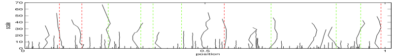
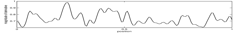
Figure 2: Hierarchical text segmentation in scale space.

5 Summary

This paper presented scale-space theory for text, adapting concepts, formulations and algorithms that were originally developed for images to address the unique properties of natural language texts. We also show how scale-space models can be utilized to facilitate a variety of NLP tasks. There are a lot of promising topics along this line, for example, algorithms that scale up the scale-space implementations towards massive corpus, structures of the semantic networks that enable efficient or even close-form scale-space kernel/relevance model, and effective scale-invariant descriptors (e.g., named entities, topics, semantic trends in text) for texts similar to the SIFT feature for images [Lowe, 2004].

References

- [Beeferman et al., 1999] D. Beeferman, A. Berger, and J. Lafferty. 1999. Statistical models for text segmentation. Machine Learning, 34:177–210.
- [Iyer and Ostendorf, 1996] R. Iyer and M. Ostendorf. 1996. Modeling long distance dependence in language: Topic mixtures vs. dynamic cache models. IEEE Transactions on Speech and Audio Processing, 7(1):30–39.
- [Jelinek et al., 1991] F. Jelinek, B. Merialdo, S. Roukos, and M. Strauss. 1991. A dynamic language model for speech recognition. HLT ’1991, pages 293–295.
- [Lebanon et al., 2007] G. Lebanon, Y. Mao, and J. Dillon. 2007. The locally weighted bag of words framework for document representation. JMLR, 8:2405–2441.
- [Lindeberg, 1994] T. Lindeberg. 1994. Scale-space theory: A basic tool for analysing structures at different scales. Journal of Applied Statistics, 21(2):224–270.
- [Lowe, 2004] D. Lowe. 2004. Distinctive image features from scale-invariant keypoints. IJCV, 60(2):91–110.
- [Manning and Schuetze, 1999] C. Manning and H. Schuetze. 1999. Foundations of Statistical Natural Language Processing. MIT Press.
- [Mei et al., 2008] Q. Mei, D. Zhang, and C. Zhai. 2008. A general optimization framework for smoothing language models on graph structures. In SIGIR ’2008, pages 611–618.
- [Metzler and Croft, 2005] D. Metzler and W. Croft. 2005. A markov random field model for term dependencies. In SIGIR ’2005.
- [Tellex et al., 2003] S. Tellex, B. Katz, J. Lin, A. Fernandes, and G. Marton. 2003. Quantitative evaluation of passage retrieval algorithms for question answering. In SIGIR ’2003.
- [Witkin, 1983] A. Witkin. 1983. Scale-space filtering. In IJCAI ’1983, pages 1019–1022.
- [Yang and Hu, 2008] S. Yang and B. Hu. 2008. Feature selection by nonparametric bayes error minimization. In PAKDD ’2008, pages 417–428.
- [Yang and Zha, 2010] S. Yang and H. Zha. 2010. Language pyramid and multi-scale text analysis. In CIKM ’2010, pages 639–648.
- [Zhai and Lafferty, 2004] C. Zhai and J. Lafferty. 2004. A study of smoothing methods for language models applied to information retrieval. ACM TOIS, 22(2):179–214.