Universality in voting behavior: an empirical analysis

Abstract

Election data represent a precious source of information to study human behavior at a large scale. In proportional elections with open lists, the number of votes received by a candidate, rescaled by the average performance of all competitors in the same party list, has the same distribution regardless of the country and the year of the election. Here we provide the first thorough assessment of this claim. We analyzed election datasets of 15 countries with proportional systems. We confirm that a class of nations with similar election rules fulfill the universality claim. Discrepancies from this trend in other countries with open-lists elections are always associated with peculiar differences in the election rules, which matter more than differences between countries and historical periods. Our analysis shows that the role of parties in the electoral performance of candidates is crucial: alternative scalings not taking into account party affiliations lead to poor results.

I Introduction

We know from statistical physics that systems of many particles exhibit, in the aggregate, a behavior which is enforced by a few basic features of the individual particles, but independent of all other characteristics. This result is particularly striking in critical phenomena, like continuous phase transitions and is known as universality binney92 . Empirical evidence shows that a number of social phenomena are also characterized by simple emergent behavior out of the interactions of many individuals. The most striking example is collective motion helbing01 ; helbing02 ; vicsek12 . Therefore, in the last years a growing community of scholars have been analyzing large-scale social dynamics and proposing simple microscopic models to describe it, alike the minimalistic models used in statistical physics. Such scientific endeavour, initially known by the name of sociophysics ball04 ; buchanan07 ; castellano09 , has been meanwhile augmented by scholars and tools of other disciplines, like applied mathematics, social and computer science, and is currently referred to as computational social science lazer09 .

Elections are among the largest social phenomena. In India, USA and Brazil hundreds of million voters cast their preferences on election day. Fortunately, datasets can be freely downloaded from institutional sources, like the Ministry of Internal Affairs of many countries. Therefore, it is not surprising that elections have been among the most studied social phenomena of the last decade fortunato12a . By now, several aspects of voting behavior have been examined, like statistics of turnout rates borghesi10 ; borghesi12 , detection of election anomalies baez06 ; klimek12 , polarization and tactical voting in mayoral elections araripe06 ; araujo10 , the relation between party size and temporal correlations andresen07 , the relation between number of candidates and number of voters mantovani11 , the emergence of third parties in bipartisan systems romero11 , the correlation between the score of a party and the number of its members schneider05b , the classification of electoral campaigns sadovsky07 , etc.

The most studied feature is the distribution of the number of votes of candidates costafilho99 ; bernardes02 ; costafilho03 ; lyra03 ; gonzalez04 ; situngkir04 ; sousa05 ; morales06 ; travieso06 ; fortunato07 ; gradowski08 ; araripe09 ; hernandez-saldana09 ; chou09 ; banisch10 . In the first analysis by Costa Filho et al. costafilho99 , the distribution of the fraction of votes received by candidates in Brazilian federal and state elections seems to decay as a power law with exponent $-1$ in the central region. Following this finding several similar analyses have been performed on election data of various countries, like India gonzalez04 , Indonesia situngkir04 and Mexico morales06 .

However, Fortunato and Castellano observed that the analysis by Costa Filho et al. treats all candidates equally, neglecting the role of the party in the electoral performance fortunato07 . This assumptions appears too strong and unjustified, as the final score of the candidate is likely to depend on whether his/her party is popular or not. For this reason Fortunato and Castellano argued that characterizing and modelling the competition of candidates of the same party is more promising, as the performance of the candidates would be mostly depending on their own activity, rather than on external factors. Such competition occurs in a peculiar type of voting system, viz. proportional elections with open lists, where people may vote for a party and one or more candidates. In this system, people may actually choose their representatives by voting directly for them, whereas the number of candidates entering the Parliament for a given party typically depends on the strength of the party at the national and/or regional level. In these elections, it was found that the distributions of the number of votes of a candidate, divided by the average number of votes of all party competitors in the same list, appear to be the same regardless of the country and the year of the election fortunato07 . This claim has been recently disputed by Araripe and Costa Filho, who found that the universal curve computed in Ref. fortunato07 does not follow well the profile of the distribution of Brazilian elections, which are also proportional and with open lists.

Here we carry out the first comprehensive analysis of the distribution of candidates’ performance, using election results of 15 countries. We focus on proportional elections, as they feature the open-list system that allow voters to choose their representatives, enabling a real competition between candidates. We conclude that the relative performance, i.e. the ratio between the number of votes of a candidate and the average score of his/her party competitors in a given list has indeed the same distribution for countries with similar voting systems, and that discrepancies from the universal distribution emerge when the election has markedly different features (e.g. large districts, compulsory voting and weak role of parties in Brazil). We also show that party affiliations cannot be neglected: statistics of the absolute performance of candidates of different parties, like that investigated in the original analysis by Costa Filho et al., do not compare well between countries.

II Results

II.1 Proportional elections

The electoral system we wish to study is proportional representation (PR) Villodres06 . We analyze data from parliamentary elections of $15$ countries: Italy (before 1992), Poland, Finland, Denmark, Estonia, Sweden, Belgium, Switzerland, Slovenia, Czech Republic, Greece, Slovakia, Netherlands, Uruguay and Brazil. The basic principle is that all voters deserve representation and all political groups deserve to be represented in legislatures in proportion to their strength in the electorate. In order to achieve this ‘fair’ representation, the country is usually divided into multi-member districts, each district in turn allocating a certain number of seats. Most countries having a PR system use a party list voting scheme to allocate the seats among the parties – each political party presents a list of candidates for each district. On the ballot the voters indicate their preference to a political party by selecting one or more candidates from the list. The number of seats assigned to each party in a district is proportional to the number of votes. The party list systems can be categorized into open, semi-open and closed.

Open lists

Open lists enable voters to express their preference not only among parties but also among candidates. A party presents an unordered, random or alphabetically ordered list of candidates. Voters choose one or more candidates, and not the party. The position of each candidate depends entirely on the number of votes that he/she receives. In this category, we have studied data from Italy (before 1994, when a new system was introduced), Poland, Finland, Denmark, Estonia (since 2002), Greece, Switzerland, Slovenia, Brazil, Uruguay.

Semi-open lists

Semi-open lists impose some restrictions on voters directly or indirectly. The voter votes for either a party or a candidate within a party list. The parties usually put up a list of candidates according to their ‘initial’ preference, which depends on internal party rankings, etc. Candidates conquer parliamentary seats in the order they are ranked in the list, from the first to the last. However, if a candidate gets a number of votes exceeding a threshold, then he/she climbs up the ranking even if he/she was initially at the bottom of the list. The final order of the candidates is decided based on the ‘initial’ ordering and the actual votes received by the candidates. Sweden, Slovakia, Czech Republic, Belgium, Estonia (until 2002) and Netherlands fall in this category.

Closed lists

In the closed list system the party fixes the order in which the candidates are listed and elected. The voter casts a vote to a party as a whole and cannot express his/her preference for any candidate or group of candidates. The representatives are then selected as they appear on the list, in the order defined before the elections. Countries voting with this system include Russia, Italy (since 2006), Spain, Angola, South Africa, Israel, Sri Lanka, Hong Kong, Argentina, etc. We did not consider this type of elections in our analysis, as there is no real competition between the candidates.

The allocation of seats to the parties takes place according to some pre-defined method, e.g. d’Hondt, Hagenbach-Bischoff, Sainte-Laguë, or some modified version of these colomer04 .

II.2 Distribution of candidates’ performance: open lists

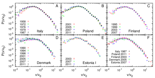
Figure 1: Distribution of electoral performance of candidates in proportional elections with open lists, according to FC scaling. Italy (until 1992), Poland, Finland, Denmark and Estonia (after 2002) follow essentially the same rules, which is reflected by the data collapse of panel F. The historical evolution of the countries does not seem to affect the shape of the distribution (panels A to E).

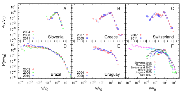
Figure 2: Same analysis as in Fig. 1, for Slovenia, Greece, Switzerland, Brazil and Uruguay. Curves are fairly stable at the national level, but they do not compare well across countries and with the universal curves of Fig.1 (represented in panel F by the distribution for the Italian elections in 1987). Such discrepancies are likely to be due to the different election rules of these countries as compared to each other and to the ones examined in Fig. 1, although they all adopt open lists.

In every proportional election, the country is divided into districts and each party presents a list with $Q$ candidates. Voters typically choose one of the parties and express their preference among the candidates of the selected party. The seat allocation depends on the country (see Section A of Appendix) and has a large influence on how voters choose who they will vote for. The data sets we considered contain information about the number of votes $v_{i}$ that each candidate $i$ received and the number of candidates $Q_{i}$ of the party list $l_{i}$ including candidate $i$. From this information one can derive the total number of votes $N_{l_{i}}$ collected by the $Q_{i}$ candidates of list $l_{i}$. By summing over all party lists in the district $D^{i}$ of candidate $i$ we obtain the number of votes $N_{D^{i}}$ in the district. The total number of votes cast during the whole election is indicated as $N_{T}$.

Our analysis consists in computing the probability distribution of the number of votes received by candidates, suitably normalized. We use the following normalizations:

• The scaling by Fortunato and Castellano fortunato07 , where the number of votes $v^{i}$ of a candidate is divided by the average number of votes $v_{0}=N_{l_{i}}/Q^{i}$ of all candidates in his/her party list. We shall indicate it as FC scaling.

• The scaling by Costa Filho, Almeida, Andrade and Moreira (CAAM) costafilho99 , where one considers the fraction of votes received by a candidate. Since it is unclear to us what one exactly means by that, we consider two possible normalizations: a) the fraction of the total votes in the district, $v^{i}/N_{D^{i}}$; b) the fraction of the total votes in the country $v^{i}/N_{T}$. We shall refer to them as to CAAMd and CAAMn, respectively. We rule out the fraction of votes in the party list because the authors made clear that they do not consider party affiliations. The most sensible definition appears the normalization at the district level, which will be thus reported here. The results for CAAMn are shown in the Appendix (Figs. B.1, B.2, B.3).

The universality discovered in Ref. fortunato07 referred to elections held in Finland, Poland and Italy in various years. Here we confirm the result with a larger number of data sets (Fig. 1). Panels A, B and C display the distributions for Italy, Poland and Finland, respectively, in different years. The stability of the curve within the same country is remarkable, especially on the tail. In panel F we compare the distributions across the countries, yielding the collapse found in Ref. fortunato07 . Elections data in Denmark and Estonia (detailed in panels D and E), appear to follow the universal curve as well. We indicate this class of countries as Group U in the following. In Ref. fortunato07 it was shown that this universal curve is very well represented by a log-normal function.

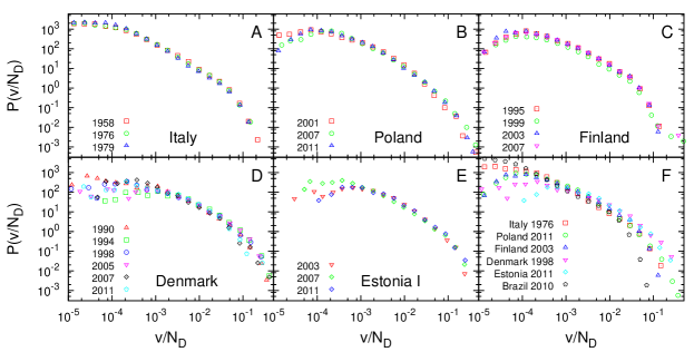
Figure 3: Same analysis as in Fig. 1, with CAAMd scaling. Curves are stable at the national level, but they do not compare well across countries.

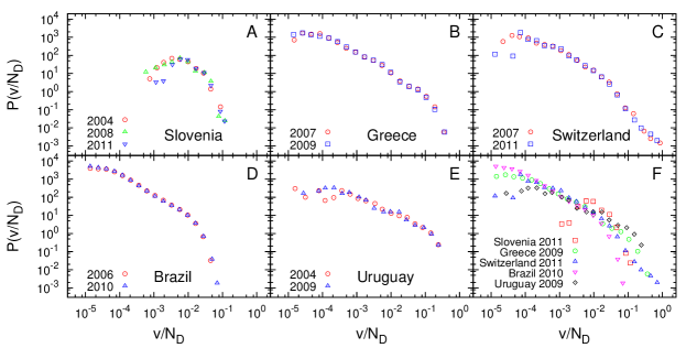
Figure 4: Same analysis as in Fig. 2, with CAAMd scaling. Curves are stable at the national level, but they do not compare well across countries.

Italy (until 1992), Poland, Finland, Denmark and Estonia (after 2002) use open lists Villodres06 , in which voters can express their preference toward certain candidates within the party list and have a direct influence on the list ordering. These lists use the plurality method for the allocation of the seats within the party lists: candidates with the largest number of nominative votes are declared elected. There are just small differences in the number of candidates that a voter can indicate, the ordering of the candidates on the ballot, but the systems are basically the same, justifying the observed universality.

Other countries using open lists are Slovenia, Greece, Switzerland, Brazil, Uruguay. The results of the FC scaling are illustrated in Fig 2. While there is a historical persistence of the distribution at the national level, the curves do not really follow a common pattern, and do not match well the behavior of the universal distribution found for Italy, Poland, Finland, Denmark and Estonia. We distinguish here two classes of behaviors: Slovenia, Greece and Switzerland are characterized by a pronounced peak at $v/v_{0}=1$, and their tails match each other quite well. Brazil and Uruguay exhibit a monotonic pattern, quite different from the other three curves. The Brazilian curve follows quite closely the profile of the universal curve of Fig. 1 on the tail ($v/v_{0}>1$).

We conclude that open list systems do not guarantee identical distributions, but can be grouped in classes of behaviors. A close inspection of the election systems, however, may explain why we observe discrepancies. Slovenia divides its territory into eight districts which in turn are partitioned into $11$ electoral units, each giving one candidate in the district. The voters can cast the vote for any of the candidates in the district, but the election of the candidate depends on the number of votes he/she won in his/her unit, i.e. the performance of the candidate in the unit is more important than the number of votes won in the district, which may affect both the candidates’ campaigns and the voters’ choices.

Greece uses a very complex seat allocation method among party lists and individual candidates. Although the ranking of the candidates on the list and the seats reallocation depends on the number of votes collected by the candidate, if one of the candidates happens to be the head of a party or a current or ex Prime Minister he/she is set automatically at the top of the party list, regardless of his/her electoral performance. Additionally, voting is compulsory, so many people cast a vote because they have to, without an informed opinion and/or motivation to participate in the election.

In Switzerland, voters may cast as many votes as there are seats in the district. They may vote for all members of the list, or for candidates of more than one party. Voters are also allowed to cast two votes per candidate. This type of list is classified as free list.

In Brazil, like in Greece, voting is compulsory, and we cannot exclude that this plays a role on the shape of the distribution. In addition, each state is just one district, which then comprises a number of voters orders of magnitude larger than the typical districts in all other elections. This explains why the Brazilian curve spans a much larger range of values for the performance variable than all other curves. The huge number of voters in the same district also explains why parties present very long lists of candidates (often with over one hundred names). Finally, the role of parties is very weak; the political constellation frequently changes, with new parties being created and old ones being reshaped.

In Uruguay voters cannot choose candidates, but lists of candidates presented by the parties, the so-called sub-lemas. Therefore our analysis focuses on the distribution of performance of sub-lemas, instead of that of single candidates.

Figs. 3 and 4 show the analogues of Figs. 1 and 2 obtained by using CAAMd scaling. The historical stability of the corresponding distributions at the national level holds, however the comparison across countries is poor: curves appear to cross, not to collapse (panel F). According to Costa Filho et al. costafilho99 the central part of the Brazilian curve follows a power law, with exponent close to $1$; power law fits of the central region of the other distributions yield exponents sensibly different from each other, which confirms the crossing of the curves (see Table C.1 of Appendix). In particular, we cound not identify any portion of the Polish curve resembling a power law. We conclude that the fraction of votes $v/N_{D}$ collected by a candidate in his/her electoral district does not follow the same probability distribution in different countries, not even when they have essentially identical voting schemes, as in Figs. 1 and  3.

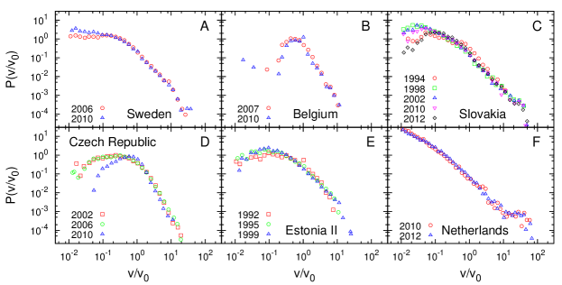
Figure 5: Distribution of electoral performance of candidates in proportional elections with semi-open lists, according to FC scaling. Voters may express preferences for the candidates, but this plays a role for the final seat assignments only if the number of votes obtained by a candidate exceeds a given threshold, which varies from a country to another. At the national level curves are mostly stable, significant discrepancies correspond to changes in the election rules, like in Slovakia (C), Czech Republic (D) and Estonia (E). The apparent power law of the Dutch curve (F) might be generated by a rich-gets-richer mechanism, since the threshold is very high (10% at the national level) and voters typically tend to support the candidates based on their popularity. We stress that Estonia since 2002 has adopted open lists, which is why distributions of Estonian elections after 2002 are illustrated in Figs. 1 and 2 (labeled as Estonia I).

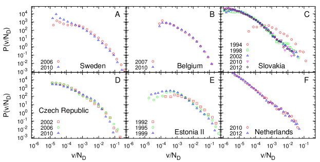
Figure 6: Same as Fig. 5, with CAAMd scaling.

II.3 Distribution of candidates’ performance: semi-open lists

The other countries we considered use semi-open lists, with different thresholds for the number of preferences that candidates are required to collect in order to secure a seat in the Parliament. The higher the electoral quota is, the harder is for a candidate to reach the required number of votes. In this case the position of the candidate within the party, as it appears on the ballot, has more influence on his/her final rank than the number of votes he/she collected. This can drastically effect the motivation of the candidate to lead a personal campaign. Also, high quotas diminish the influence of the voter on the final list ordering, which affects both the degree of a candidate’s involvement in his/her personal campaign and the way people cast their preference votes. Therefore there is hardly an open competition between candidates, and this may be reflected in the shape of the distribution of performance. Figure 5 shows the probability density distributions for different countries with semi-open lists, according to FC scaling. The elections in Czech Republic held in $2010$ had the lowest electoral quota and $P(v/v_{0})$ (Fig. 5D) turns out to be very similar to the curve obtained for Greek elections (Fig. 3B). The country with the highest electoral quota are the Netherlands, where each candidate has to win $10\%$ of votes cast on the national level in order to be directly elected. Voters in Netherlands have little or no influence on the ordering of candidates, which is essentially frozen by the party, and they often vote for the top-ranked candidate and the first several names on the list, as they are the most popular and appreciated members of the party. This resembles the rich-gets-richer effect, which is characterized by power-law behavior of the distribution of the relevant quantities Eggenberger23 ; Simon55 ; Merton68 ; Price76 ; Albert02 . Indeed, the distribution of performance of Dutch candidates follow an approximate power-law behavior over most of the range of the performance $v/v_{0}$ (Fig. 5F).

Besides the values of the electoral threshold, these countries also differ in the number of nominative preferences a voter can cast, in the size and number of multi-member districts, as well as in the electoral formula that determines the final rankings (see Section A of Appendix). Any change in the electoral system, i.e. these several factors, might influence the shape of $P(v/v_{0})$. For instance, in $1994$ Slovakia changed the number of multi-member districts, leading to appreciable changes in the shape of the distribution (Fig. 5C). The change in the electoral quota and the number of nominative votes decided in Czech Republic in $2006$, may be the responsible for the variation of the curve before and after that year (Fig. 5D). The transition from semi-open to open lists introduced in Estonia in $2002$, might explain why the curves before and after that year look different (Fig. 1E versus Fig. 5E). Interestingly, after the introduction of open lists in Estonia, the distribution of performance matches the universal distribution of the other countries with similar election systems (Fig. 1F), while before $2002$ we find clear discrepancies.

The corresponding distributions with CAAMd scaling also show marked differences between different countries (Fig. 6).

II.4 Estimating the similarity of the distributions

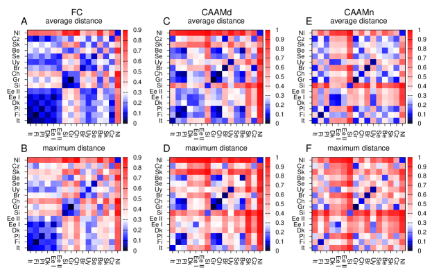
Figure 7: Quantitative assessment of the similarity between distributions at the national level and between countries. The matrices in the top row indicate the values of the average K-S distance between datasets of different countries. On the bottom row the maximum distances are reported. Each column corresponds to one of the three types of distributions we have examined, by using FC, CAAMd and CAAMn scaling. A color code is adopted to better distinguish the low values of the distance (indicated by the blue), indicating a big similarity between the curves, from the larger values, corresponding to poor collapses. The bluish square on the bottom left of the matrices obtained via FC scaling confirm that the distributions of those countries are pretty close to each other, as illustrated in Fig. 1F. Conversely, the similarity between distributions obtained via CAAMd and CAAMn scaling appears rather modest for most pairs of countries.

So far the estimation of the agreement or disagreement of different curves has been basically visual. In this section we would like to attempt a quantitative assessment of this issue. We build two matrices, whose entries are the values of the average distance $D_{avg}$ and the maximum distance $D_{max}$ between the distributions for any pair of countries for which we gathered election data (see Methods). The dissimilarity values for elections in the same country are reported on one diagonal of the matrix. Since we have adopted three different types of scaling for the electoral performance of candidates, FC, CAAMd and CAAMn, we end up with six matrices, which are illustrated in Fig. 7. In each column we display the pair of matrices corresponding to one type of scaling, the first row contains the average distances, the second row the maximum distances. We built $16\times 16$ matrices, even if we studied 15 countries, because we considered two sets of elections for Estonia, because of their transition from semi-open lists (Ee II) to open lists (Ee II), which took place in 2002.

Potential data collapses are indicated by low values of $D_{avg}$ and $D_{max}$, which are easier to spot by using a color code, as we did in the figure. Numerical values are listed in the Appendix in the Tables C.2, C.3, C.4, C.5, C.6, C.7. Dark squares (black-blue) correspond to the lowest values of $D_{avg}$ and $D_{max}$, so to very similar distributions. The data collapse for the countries of Group U (Fig. 1F) is illustrated by the bottom left block of A and B. Interestingly, we see that only the Estonian elections held after 2002 (Ee I) are very similar to the other curves of Group U; before 2002 Estonians used semi-open lists, the corresponding curves do not match well with the universal distribution.

We see that also the Brazilian and the Uruguayan distributions are fairly similar, on average, to the universal curve, mostly on the tail, although they considerably differ in the initial part, especially the Brazilian distributions. The strong similarity between the results of elections in the nations of Group U persists even if we consider the maximum distance (panel B), as the dark block is still there, though blurred. Slovenia and Greece appear very similar to each other but sensibly different from the other countries. The diagonal from bottom left to top right shows the values of the distance for datasets in the same country. In general, the distances are pretty low, but we also find fairly large values. These correspond to countries which introduced changes in the election rules, reflected in the shape of the distributions, as described above.

If we move to CAAMd scaling (panels C and D) the scenario is considerably worse, in that the curves are much more dissimilar to each other than the ones obtained with FC scaling. In panel C, the average distance between the countries of Group U is still low, though higher than for FC scaling (panel A), but when one moves to the maximum distance the block disappears (panel D). For CAAMn (panels E and F) the curves are even more dissimilar to each other.

We are not giving here any indication on the significance of the measured values of the K-S distance. Large values indicate with certainty that the corresponding distributions are really different curves, but low values could still have high significance. As a matter of fact, all values that we found, for all types of scaling, indicate a significant discrepancy between the corresponding distributions. However, we stress that here we are considering the whole profile of the distribution, from the lowest to the highest value of the performance variable. The most interesting part of the distributions, and the one which is likely to reflect collective social dynamics, is certainly the tail, because it is where one has the largest cascades of votes for the same individual. On the contrary, the initial part of the curve corresponds to poorly voted candidates, and there are many ways to get to such modest outcomes (like being voted solely by closest family members and friends), hardly susceptible of a mathematical modelling. But at this stage we did not want to identify the most “interesting” part of the distribution by constraining the range of the variable, which is always tricky. Therefore we decided to compare the full distributions.

We finally remark that in social dynamics one can hardly get the same striking data collapses obtained in physical systems and models. Even if the social atom hypothesis implies that just a few features of the social actors and their interactions determine the large-scale behavior, the complexity of human nature and context-dependent factors may still have some influence, albeit small. For instance, in the Polish distributions of Fig. 1B there is a hump for $v/v_{0}\approx 5$, which occurs systematically at the national level, but which is absent in the other distributions of the same class. Therefore, obtaining the agreement of the distributions shown in Fig. 1F, despite all differences between countries and historical ages, is truly remarkable.

III Discussion

We have performed an empirical analysis of elections held in 15 countries in various years. We focused on the competition between candidates, which is a truly open competition when the voters can indicate their favourite representatives in the ballot and candidates with the largest number of votes are ranked the highest. This occurs in proportional elections with open lists. Of the countries for which we found data, 10 adopt open lists. Five of them (Group U), Italy, Finland, Poland, Denmark and Estonia (since 2002) have very similar election rules, the other five are characterized by important differences (e.g. compulsory vote, huge districts and weak role of parties in Brazil), which are likely to affect the behavior of voters and candidates, leading to measurable differences in the statistical properties of the electoral outcomes. Indeed, the distribution of the number of votes received by a candidate, normalized by the average number of votes gained by his/her competitors in the same party list, seems to be the same for the nations of Group U, while there are marked differences from the curves obtained from the other countries. This result, originally found by Fortunato and Castellano for Italy, Finland and Poland fortunato07 , is confirmed here on a much larger data collections and holds for Denmark and Estonia as well.

Different patterns are found for countries adopting semi-open lists, in which in principle voters can choose the candidates, but the main ranking criterion is still imposed by their party, regardless of the final electoral score of the candidate, unless it exceeds a given threshold. In this system the competition among the candidates is therefore not really open, and it is no wonder that the distribution of electoral performance does not follow the profile of the curves of Group U.

In general we found that the shape of the distribution is much more sensitive to the specific election rules adopted in the countries than to the historical and cultural context where the election took place. This is evident when one considers the evolution in time of distributions of any given country, which remain essentially identical even after many years, if the voting system does not change, but display visible variations following the introduction and/or modification of election rules as it happened in Estonia in 2002, Slovakia in 1994, Czech Republic in 2006. The case of Estonia is spectacular: before 2002 it used semi-open lists, and the distributions of relative performance of a candidate with respect to his/her party competitors did not compare well with the curves of the other countries of Group U. After the introduction of open lists, instead, the distributions became very similar to the universal curve. Such sensitivity of the distributions might allow to detect anomalies, e.g. large-scale fraud, in future elections baez06 ; klimek12 .

Our analysis proves that the success of a candidate, measured by the number of votes, strongly depends on the party he/she belongs to, and that only when one considers the competition among candidates of the same party universal signatures may emerge. Indeed, neglecting the party affiliation does not seem to take us very far: the two party-independent normalizations we have considered, following the procedure by Costa Filho et al. costafilho99 ; costafilho03 ; araripe09 , do not seem to reveal strong common features among distributions of different countries, not even when the latter follow nearly identical election schemes (e.g. the nations of Group U).

IV Methods

IV.1 Election data

Here we consider the data sets for parliamentary elections from $15$ countries with open and semi-open lists: Italy (1958, 1972, 1976, 1979 and 1987)  ItalyData , Poland (2001, 2005, 2007 and 2011)  PolandData , Finland (1995, 1999, 2003 and 2007)  FinlandData , Denmark (1990, 1994, 1998, 2001, 2005, 2007 and 2011)  DenmarkData , Estonia (1992, 1995, 1999, 2003, 2007 and 2011)  EstoniaData , Slovenia (2004, 2008 and 2011)  SloveniaData , Greece (2007 and 2009)  GreeceData , Switzerland (2007 and 2011)  SwissData , Brazil (elections for state deputies in 2002, 2006 and 2010)  BrazilData , Uruguay (2004 and 2009)  UruguayData , Sweden (2006 and 2010)  SwedenData , Belgium (2007 and 2010)  BelgiumData , Slovakia (1994, 1998, 2002, 2010 and 2012)  SlovakiaData1 ; SlovakiaData2 , Czech Republic (2002, 2006 and 2010)  CzechData and the Netherlands (2010 and 2012) NetherlandsData . Further details and sources for each file are given in Table C.8 in Appendix, while the compiled and cleaned data maybe be downloaded at http://becs.aalto.fi/en/research/complex_systems/elections/.

IV.2 Comparing distributions

We use the Kolmogorov-Smirnov (K-S) distance NR to measure the dissimilarity of two empirical distributions. The K-S distance $D$ is defined as the maximum value of the absolute difference between the corresponding cumulative distribution functions, i.e.

$$D=\max_{x}|S_{N_{1}}(x)-S_{N_{2}}(x)|$$ (1)

where $S_{N_{1}}(x)$ and $S_{N_{2}}(x)$ are the cumulative distributions for two data sets of size $N_{1}$ and $N_{2}$.

Since we have multiple datasets for each country, in order to compute the dissimilarity of the distributions at the national level and across countries we proceed as follows. For a given country $X$ we compute the distance between any two distributions for elections of $X$. For a pair of countries $X$ and $Y$ we compute the distance between any pair of distributions $P_{X}$ and $P_{Y}$, corresponding to one dataset of $X$ and one of $Y$, respectively. In both cases we take the average $D_{avg}$ and the maximum $D_{max}$ of the resulting values. In this way we estimate the average and the maximum distance between distributions of the same country and between distributions of two different countries.

Appendix A Description of election systems

Italy

During 1948 to 1992, the members of the Chamber of Deputies (Camera dei Deputati) were elected by proportional representation (PR) in multi-member electoral districts, except in Valle d’Aosta where one member was elected by simple majority. Over this legislative period, Italy used an open-list PR system in which voters could decide to use as many as 3 (4 for very large districts) preference votes for individual candidates on the party list of their choice. However, in 1992 this number was limited to unity. In each constituency, seats were divided between open lists using the largest remainder method with the Imperiali quota, and the remaining votes and seats were transferred to the national level, where special closed lists of national leaders received the last seats using the Hare quota.

Poland

The lower chamber of the Polish parliament, the Sejm, has $460$ seats out of which $391$ are elected in the multi-member districts and $69$ at the national level. The seats within the district are allocated to a party or independent list according to d’Hondt method, and reallocation to the candidates on each list is done according to plurality rule.

Finland

The Finnish parliament, Eduskunta, has $200$ seats, distributed among $15$ multi-member districts. The candidates are nominated by a political party. A political party presents a list for each district, with at least $14$ candidates. In Finland there is no electoral threshold and all seats are allocated within the electoral constituencies. The voter is presented with the ballots from each party, and he/she cast a vote for one candidate only, expressing this way a preference toward a certain candidate, but also towards a certain party. The allocation of the seats is according to d’Hondt constituency list system.

Denmark

The parliament of the Kingdom of Denmark, the Folketing, is composed of $179$ members directly elected by a two-tier, six-stage proportional representation system. $135$ of the total $175$ members that represent metropolitan Denmark are chosen in multi-member electoral districts grouped into three electoral regions, while the remaining $40$ seats are allocated to ensure proportionality at a national level. Voters may cast a ballot for a district party list, or for a specific candidate. From $1970$ to $2005$ the seats within the constituencies were distributed according to the modified Sainte-Laguë method of PR, while since $2007$ the seats are distributed according to the d’Hondt or largest average method of PR. The seats on the national level are apportioned among political parties that obtain at least one district seat, or obtained as many votes as on average were cast per constituency seat in at least two of the three regions, or at least two percent of all valid votes cast at the national level. The total number of seats to which each cartel is entitled is determined using the d’Hondt method. From this total number is then subtracted the number of constituency seats won by associated lists within each district. The difference gives the number of the forty supplemental seats to which the party is entitled. Seats awarded on the national level are reallocated to each party’s component constituency lists by a two-step procedure. Seats are first allocated to regions, by the Sainte-Laguë method. Then, within regions, they are allocated to constituencies by another divisor method. These seats are then re reallocated to each list’s candidates, by three different procedures.

Estonia

We consider the data from the elections to the Estonian parliament (Riigikogu) for the period of two decades ($1992$-$2012$) during which there were two reforms in the electoral system in $1994$ and $2002$ renwick2011 . Keeping in mind the years of these reforms, the data sets for Estonian elections can be categorized into three groups: $1992$ as the first group, the second consists of the data from the elections held in $1995$ and $1999$, and in the third we consider elections after the second reform, that of $2003$. The rules used in elections in $1992$ were partly similar to those used in Finland grofman1999 . The country was divided into $12$ multi-member districts whose magnitudes ranged from five to thirteen seats, whereas the whole Estonian parliament consists of $101$ members. Each party presented a list of candidates and voters voted for an individual candidate. Candidates who received a Hare quota were certified as personally elected. The remainder of votes were added by the list, and if full quota materialized, the top voted candidates on the list received district seats. Unlike Finland, where the seats are allocated in the district, the remained unallocated seats were compiled nationwide and appointed to closed lists of parties that received at least five percent of the votes on national level. For the allocation on the national level the quasi-d’Hondt quota was used grofman1999 . This kind of system led to selection of candidate which had only $51$ personal votes. For this reasons, a restriction for district seats was introduced for the elections held in $1995$: in order to be chosen, a candidate had to win at least the number of votes equal to $0.1$ of quota. The reform in $2002$ was related to lists at the national level, the ordering of the candidates was according to the number of their personal votes. In this sense the later reform, the transition from semi-open to open lists led to a greater personalization of the electoral system in Estonia renwick2011 .

Slovenia

In Slovenia, the deputies of the National Assembly (Državni zbor), with the exception of the two representatives of minorities, are elected by proportional representation, with a $4\%$ electoral threshold required at the national level. The country is divided into eight territorial constituencies, each represented by eleven elected deputies. For the elections of the representatives of the Italian and Hungarian ethnic communities, two special constituencies are formed, one for each minority. The deputies representing the minorities are elected on the basis of the majority principle. The seat allocation within the districts is as follows: each list gets as many seats as there are whole Hare quotas contained in its vote within the district. Seats unallocated within the districts are aggregated at the national level and distributed by PR-d’Hondt rule, on the basis of each party remainder vote (the sum of all remainders from associated constituency lists). Only lists which won at least three seats are eligible to participate in this step of seat allocation. The party seats won on the national level are reallocated to the lists according to their ranking. The lists within the party are ranked according to their remainder is expressed as a fraction of the quota in its constituency. The lists from constituencies all of whose seats have already been allocated are not considered in the apportionment of national seats. The seats awarded to the lists are reallocated to each list’s candidates as follows and candidates on each list are associated with one (or two) geographically defined sub-districts. The candidates on each list are ranked in terms of the percentage of the total vote each has received in his or her sub-district. The top candidates on the list get the seats to which their list is entitled.

Greece

The Hellenic Parliamnet is composed of $300$ deputies elected for four-year term through reinforced proportional representation system. Greece is divided into $56$ districts, out of which $48$ have more than one representatives in the Parliament. The winning party on the national level in Greece receives a majority bonus of $40$ in $2007$ ($50$ in $2009$), while the remaining $260$ ($250$ in $2009$) seats are distributed by the largest remainder method (Hagenbach-Bischoff) of proportional representation (PR) on a nationwide basis among parties polling at least $3\%$ of the vote. The voters can express their preference toward certain candidates on the the party list. The number of preference votes depends on the number of seats in constituency. Single-member seats were filled by the plurality or first-past-the-post method, in which the candidate obtaining the largest number of votes in the constituency was elected to office. In multimember districts the seats won by party are reallocated to each list’s candidates by plurality. The only exception are the party heads and acting or past Prime Ministers who are automatically placed at the top of their party list.

Switzerland

The National Council (Nationalrat/Conseil National/Consiglio Nazionale/Cussegl Naziunal) is composed of $200$ members elected for a $4$-year term of office in $26$ constituencies - the cantons of Switzerland. The electors have as many votes as there are allocated seats for the district. These votes can be given to all candidates on a single list or to candidates from different lists. The seats apportionment within the constituency is based on Hagenbach-Bischoff method, while the list seats are assigned to the candidates with the largest vote totals within each list. Like in Poland, Finland, Denmark and Estonia, the voters have total control on who will represent them in parliament.

Brazil

In Brazil, the elections for the $513$ seats of the Chamber of Deputies (Câmara dos Deputados) of the National Congress are conducted in $27$ multi-member ($8$ to $70$ seats, based on population) constituencies corresponding to the country’s $26$ states and the Federal district, using the party-list proportional system with seats allotted according to the simple quotient and highest average calculations. The seats won by each list are in turn awarded to the candidates on the basis of preferential votes cast by the electorate. Vacancies arising between general elections are filled by substitutes elected at the same time as titular members. If no substitute is available and there remain at least 15 months before the end of the term of the member concerned, by-elections are held. Furthermore, voting is compulsory, and abstention being punishable by a fine.

Uruguay

The Chamber of Deputies (Cámara de Diputados) in Uruguay has $99$ seats allocated in $19$ multi-member districts through a list proportional representation system. The members of the Chamber are elected for $5$ year term. Voting is compulsory in Uruguay and unjustified abstention is penalized by a fine. The elections for Chamber are in the same time as the elections for the Senate and presidential elections. For each district the party can present more then one list, so called sub-lemas containing usually a pair of candidates or more. Uruguay uses the rule of the double simultaneous vote (DSV), which means that the voter must vote for one of the sub-lemas of the party he/she has chosen in a Presidential contest. The distribution of seats between political parties or cartels is decided by tallying the votes of each sub-lemas. The allocation of the seats is done according to variation of d’Hondt formula devised by Borelli. The possible remaining seats are distributed on the national level. Although the voters can not cast a vote for a single member but for the sub-lemas, we can use the quantity $v/v_{0}$ for measuring performance of the sub-lemas since the parties propose several sub-lemas which usually contain two or three names. The data we consider here, have information about the number of votes cast for each of the lists. The performance of the sub-lema is expressed as the relation between the number of votes won by sub-lema and number of votes won in average by all sub-lemas proposed by a party or cartel in the district.

Sweden

The elections to the Swedish parliament (Riksdag) uses open lists system, but unlike in countries previously discussed, the voters can choose between three different types of ballots papers: the party ballot paper which has simply the name of the party, the name ballot paper has a party name followed by a list of candidates and alternatively, a voter can take blank ballot paper and write a party name on it. Voters in Sweden can either vote for a party without expressing a preference towards any candidate, or can vote for a person on the list, thereby giving the voice to one candidate and indirectly to his/her party. Seats are allocated among the Swedish political parties proportionally using a modified form of the Saint-Laguë method. The candidates from the each party are determined according by two factors: the candidate’s ranking by their party and the number of preference votes the obtained in the elections. If the candidate receives a number of personal votes equal or greater than $8\%$ of the party’s total amount of votes, he/she will be automatically shifted to the top of the list, regardless of the previous ranking. This type of system gives the voters a degree of power in choosing candidates from the list, but not as much as in the case of Poland. This is reflected in the way people cast their votes and how the performance of the candidates are distributed.

Belgium

In Belgium, the Chamber (Kamer van Volksvertegenwoordigers/Chambre des Représentants/Abgeordnetenkammer) seats are filled in eleven constituencies. The political parties present the lists of candidates and voters can either indicate a preference for one or more of them, or vote for a party. The seats are distributed in each district among the lists that receive at least of all valid votes cast in the constituency according to d’Hondt system. The ordering of the candidates on the lists is similar to Sweden, i.e. it is a combination of party ordering and nominative votes.

Slovakia

For Slovakia we consider several election years $1994$, $1998$, $2002$, $2010$ and $2012$ during which there were three reforms of electoral system, $1998$, $1999$ and $2004$ renwick2011 . The National council (Národná rada) of the Slovakian parliament consists of $150$ members chosen for four year term on proportional representation elections. For the elections in $1994$ the country was divided into four multi-member constituencies. Each political party was nominating their candidates, by submitting the list of not more than $50$ candidates in each constituency. The voters were allowed to vote for four candidates on the list of the same party, expressing this way their preference toward certain candidates. The seat allocation among the parties within the constituency was according to the Hagenbach-Bischoff system. All parties with more than $5\%$ of the votes on national level took part in the seat distribution. Within individual political parties the mandates were distributed among candidates nominated by these parties in the order of priority of the list of candidates. If some of the candidates gained at least $10\%$ of preferential votes of the total number of votes cast for a political party within a constituency, he/she had an advantage over other candidates on the list, regardless of his/hers previously determined order. If the political party had the right to several mandates, and several candidates met the conditions specified in the previous sentence, then the candidates obtained mandates in the order which was determined by the largest number of preferential votes, cast for them. In case of equal preferential votes, the position of candidate for Deputy in the list of candidates was decisive. After the elections in $1994$, Slovakia became one, nationwide electoral constituency, where political parties or coalitions could submit lists of $150$ candidates. This semi-open list system puts elections in Slovakia between elections in Netherlands, where the voters do not have an influence on the seat allocation within the party, and countries like Finland and Poland, where the ordering of the candidates solely depends on the preference of the voters.

Czech Republic

The lower house of the Czech Republic, the Chamber of deputies (Poslanecká sněmovna) is composed of $200$ members directly elected by proportional elections. The apportionment of Chamber seats in each of the fourteen multi-member districts among competing lists is done using d’Hondt rule. In order to participate in the distribution of constituency seats, a party must obtain at least $5\%$ of all valid votes cast at the national level, while coalitions of $2$, $3$ and $4$ or more parties are required to obtain at least $10$, $15$ and $20$ percent of the vote (previously $7$, $9$ and $11$ percent) respectively. The electoral reforms of 2000 changed the number of preferences to $2$ and the seats within the list are allocated to candidates in the order in which they appear on the list, but the candidates which received at least $7\%$ (reduced from $10\%$) of the votes cast for their party list have priority in the allocation of seats, regardless of their position on the list. This was followed in the elections of 2002 and 2006. However in 2010, the preferences were set to $4$ and the amount of necessary preferences for the relevant candidate was reduced to $5\%$.

Netherlands

The House of Representatives (Tweede Kamer) has a particular way of allocating seats. Each party can represent the list of $50$ candidates ($80$ if the party had more than $15$ seats in the previous term) with predetermined ordering of the candidates. The first person on the list, list puller, is usually appointed by the party to lead its election campaign and is a candidate for the Prime Minister. Although, parties may choose to compete with the different candidates in each district, the seat allocation on the national level results in nationwide lists. Since, the voters cannot influence the ordering of the candidates, i.e. the lists are of closed types, they often vote for the list puller and first several candidates on the list, as the more popular and appreciated members of the party.

Appendix B CAAMn scaling

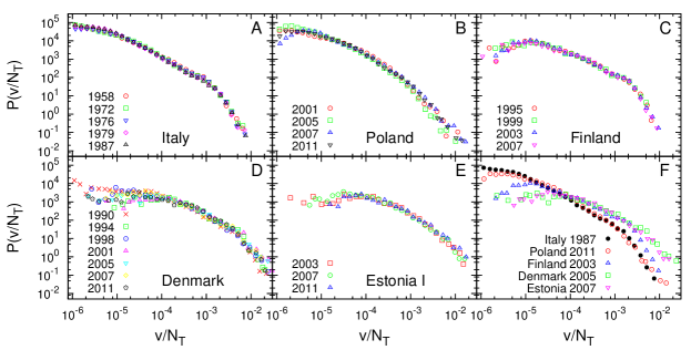
Figure B.1: Distributions of the fraction of votes obtained by a candidate within the entire country for different election years for (A) Italy, (B) Poland, (C) Finland, (D) Denmark, (E) Estonia ($2003,2007,2011$). A comparison of the scaling curves for these countries is shown in (F).

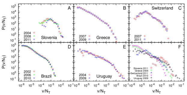
Figure B.2: Distributions of the fraction of votes obtained by a candidate within the whole country for different election years for Slovenia, ( Greece, (C) Switzerland, (D) Brazil and (E) Uruguay. A comparison of the scaling curves for these countries is shown in (F).

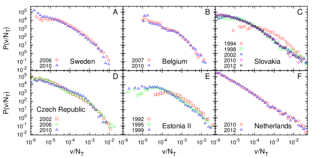
Figure B.3: Distributions of the fraction of votes obtained by a candidate within the whole country for different election years in (A) Sweden, (B) Belgium, (C) Slovakia, (D) Czech Republic, (E) Estonia (1992, 1995, 1999), and (F) Netherlands.

Appendix C Tables

Table C.1: The estimates of $\gamma$ exponent for CAAMd scaling for open-list electoral systems. For Poland and Uruguay, it is not possible to find any finite range of values for which a power-law could be fitted.

Country	Year	$x_{min}$	$x_{max}$	$\gamma$
Italy	1958	$0.00021$	$0.04871$	$-1.27(4)$
Poland		n.d.	n.d.	n.d.
Finland	1999	$0.00036$	$0.02879$	$-1.11(3)$
Denmark	2007	$0.00063$	$0.02959$	$-1.08(3)$
Estonia	2011	$0.00330$	$0.08730$	$-1.47(5)$
Greece	2007	$0.00008$	$0.03403$	$-1.10(4)$
Switzerland	2007	$0.00063$	$0.02795$	$-1.21(4)$
Brazil	2006	$0.00007$	$0.00968$	$-1.12(1)$
Uruguay		n.d.	n.d.	n.d.

Table C.2: FC scaling: Average distance $D$ between datasets from different countries.

	It	Fi	Pl	Dk	EeI	EeII	Si	Gr	Ch	Br	Uy	Se	Be	Sk	Cz	Nl
It	0.03801	0.06560	0.05380	0.09199	0.07412	0.15788	0.37039	0.29121	0.45663	0.23223	0.14801	0.19722	0.28724	0.27584	0.12724	0.65437
Fi		0.02592	0.10756	0.06669	0.11274	0.16889	0.31749	0.23889	0.40258	0.25590	0.14209	0.23261	0.23913	0.30750	0.07937	0.67421
Pl			0.04236	0.12456	0.07161	0.15240	0.41216	0.33374	0.49942	0.21605	0.18217	0.17276	0.32289	0.25497	0.16750	0.64148
Dk				0.08410	0.12214	0.16958	0.31303	0.23599	0.39847	0.23272	0.13046	0.23501	0.23729	0.29784	0.09915	0.64581
EeI					0.05032	0.11546	0.40584	0.32818	0.48532	0.20248	0.13599	0.14914	0.34322	0.22991	0.17743	0.62883
EeII						0.14210	0.43881	0.36203	0.51480	0.14974	0.16591	0.11289	0.37911	0.19494	0.21826	0.56205
Si							0.06288	0.08608	0.11806	0.46576	0.33138	0.52184	0.18294	0.56076	0.25497	0.82169
Gr								0.02087	0.17273	0.39836	0.26706	0.44342	0.14608	0.48803	0.18109	0.77310
Ch									0.17259	0.53076	0.39489	0.59665	0.22172	0.63361	0.34065	0.86106
Br										0.08174	0.16535	0.12180	0.42645	0.16871	0.28469	0.43365
Uy											0.11100	0.23317	0.29583	0.27973	0.16721	0.55188
Se												0.07814	0.45601	0.14886	0.29123	0.49503
Be													0.16144	0.51014	0.18404	0.80793
Sk														0.18281	0.35344	0.45883
Cz															0.11962	0.69293
Nl																0.10844

Table C.3: FC scaling: Maximum distance $D$ between datasets from different countries.

	It	Fi	Pl	Dk	EeI	EeII	Si	Gr	Ch	Br	Uy	Se	Be	Sk	Cz	Nl
It	0.07070	0.09998	0.10859	0.16108	0.10361	0.21909	0.43408	0.31982	0.54035	0.31357	0.20025	0.24036	0.33814	0.40206	0.26237	0.69261
Fi		0.03241	0.14086	0.13231	0.13737	0.25200	0.35904	0.24493	0.46759	0.33103	0.16655	0.27059	0.26516	0.42020	0.19063	0.71052
Pl			0.05897	0.19237	0.08694	0.19499	0.47491	0.36068	0.57986	0.29779	0.24170	0.22232	0.37147	0.38301	0.29832	0.67978
Dk				0.18642	0.20043	0.30713	0.45101	0.33843	0.54346	0.34308	0.18052	0.32110	0.36328	0.44594	0.28313	0.69737
EeI					0.07077	0.18239	0.45052	0.34142	0.54968	0.28357	0.18697	0.20743	0.37557	0.36842	0.29624	0.67421
EeII						0.20064	0.55498	0.44567	0.64241	0.27050	0.26773	0.21713	0.48052	0.36279	0.40379	0.64199
Si							0.06963	0.12116	0.18554	0.55632	0.38073	0.57478	0.20762	0.66732	0.34597	0.85289
Gr								0.02087	0.23365	0.46823	0.27242	0.46320	0.16256	0.57763	0.23186	0.79092
Ch									0.17259	0.62214	0.45975	0.65662	0.34539	0.73473	0.45101	0.88318
Br										0.11955	0.23797	0.16632	0.51099	0.22314	0.43536	0.50603
Uy											0.11100	0.27942	0.31512	0.35771	0.23877	0.59656
Se												0.07814	0.49512	0.23553	0.41632	0.56354
Be													0.16144	0.62021	0.24679	0.83190
Sk														0.30812	0.54228	0.58983
Cz															0.17079	0.77514
Nl																0.10844

Table C.4: CAAMd scaling: Average distance $D$ between datasets from different countries.

	It	Fi	Pl	Dk	EeI	EeII	Si	Gr	Ch	Br	Uy	Se	Be	Sk	Cz	Nl
It	0.06929	0.24181	0.19605	0.43669	0.39816	0.37895	0.71540	0.16986	0.20398	0.15814	0.49786	0.19310	0.17631	0.51498	0.13853	0.82727
Fi		0.04488	0.09237	0.22718	0.17321	0.18166	0.54486	0.12413	0.07568	0.34413	0.38077	0.20539	0.13957	0.59584	0.31366	0.90123
Pl			0.05296	0.30310	0.24112	0.21381	0.62367	0.10381	0.05648	0.31814	0.44676	0.17102	0.07638	0.59226	0.28284	0.89917
Dk				0.14625	0.14076	0.23600	0.34091	0.28756	0.28417	0.50810	0.23662	0.40870	0.35072	0.71065	0.48959	0.93467
EeI					0.16015	0.20126	0.41525	0.26706	0.23025	0.49047	0.31402	0.35743	0.29123	0.70049	0.46403	0.94112
EeII						0.27932	0.49650	0.26027	0.20853	0.48211	0.36498	0.32008	0.25375	0.69835	0.45156	0.94359
Si							0.12409	0.55850	0.59761	0.75097	0.27246	0.70531	0.66668	0.87455	0.74770	0.98217
Gr								0.02514	0.08957	0.23211	0.37571	0.18430	0.12873	0.53297	0.22762	0.85404
Ch									0.03784	0.31057	0.40198	0.16720	0.09645	0.57467	0.27950	0.89779
Br										0.04599	0.53713	0.20996	0.31572	0.42003	0.09011	0.77025
Uy											0.07334	0.50697	0.48601	0.75089	0.54306	0.93769
Se												0.31276	0.19498	0.51565	0.20655	0.82880
Be													0.07014	0.60935	0.27882	0.92955
Sk														0.37043	0.45729	0.64184
Cz															0.14945	0.79005
Nl																0.11057

Table C.5: CAAMd scaling: Maximum distance $D$ between datasets from different countries.

	It	Fi	Pl	Dk	EeI	EeII	Si	Gr	Ch	Br	Uy	Se	Be	Sk	Cz	Nl
It	0.09564	0.31050	0.27939	0.59191	0.51746	0.56189	0.79147	0.21808	0.25947	0.20313	0.54676	0.29096	0.24784	0.59231	0.19929	0.83707
Fi		0.06399	0.12927	0.37020	0.25594	0.31480	0.60435	0.14990	0.10232	0.38160	0.40233	0.32485	0.17915	0.75149	0.40082	0.91477
Pl			0.07079	0.46116	0.33911	0.40269	0.69504	0.11828	0.07156	0.34448	0.46076	0.29170	0.13499	0.72876	0.36182	0.91553
Dk				0.27609	0.28350	0.46215	0.52053	0.38945	0.41921	0.61449	0.31473	0.61296	0.50386	0.89750	0.65247	0.95876
EeI					0.16015	0.32867	0.52946	0.32185	0.31209	0.55802	0.33626	0.53202	0.39225	0.87834	0.58936	0.95553
EeII						0.40882	0.70318	0.35761	0.36411	0.59422	0.47135	0.57410	0.44274	0.90111	0.62867	0.96391
Si							0.15834	0.60628	0.65331	0.79363	0.30116	0.81381	0.72674	0.97543	0.83624	0.98663
Gr								0.02514	0.09492	0.24590	0.38503	0.23799	0.13999	0.62957	0.28286	0.86564
Ch									0.03784	0.32906	0.41469	0.27331	0.10927	0.69802	0.34844	0.92066
Br										0.04599	0.55228	0.37209	0.36614	0.46050	0.18873	0.78936
Uy											0.07334	0.56762	0.49001	0.86231	0.59356	0.94393
Se												0.31276	0.30932	0.74055	0.38563	0.87916
Be													0.07014	0.75194	0.36306	0.93611
Sk														0.82481	0.56383	0.93643
Cz															0.20000	0.82044
Nl																0.11057

Table C.6: CAAMn scaling: Average distance $D$ between datasets from different countries.

	It	Fi	Pl	Dk	EeI	EeII	Si	Gr	Ch	Br	Uy	Se	Be	Sk	Cz	Nl
It	0.09735	0.40966	0.14123	0.58838	0.61612	0.58557	0.85043	0.11092	0.41552	0.11946	0.51910	0.20152	0.39650	0.25389	0.13287	0.45861
Fi		0.04351	0.35011	0.23342	0.24521	0.21334	0.64307	0.31078	0.13590	0.47827	0.24283	0.34281	0.31376	0.31712	0.33150	0.74166
Pl			0.09321	0.55354	0.57673	0.52816	0.87547	0.12517	0.31186	0.21890	0.51622	0.18065	0.34107	0.18941	0.14757	0.55727
Dk				0.12727	0.10739	0.23872	0.45690	0.49039	0.34408	0.62871	0.13951	0.54174	0.45328	0.44034	0.50761	0.82775
EeI					0.08995	0.23476	0.47561	0.51604	0.36519	0.65453	0.14583	0.56573	0.47355	0.45637	0.53249	0.85558
EeII						0.31559	0.56396	0.48834	0.29685	0.63564	0.26306	0.51877	0.45609	0.45362	0.50424	0.84092
Si							0.12035	0.78621	0.71714	0.88896	0.42180	0.86111	0.75142	0.75679	0.81878	0.95440
Gr								0.04070	0.32655	0.17752	0.43189	0.16606	0.36930	0.20312	0.11543	0.46402
Ch									0.09460	0.49885	0.32350	0.30518	0.32525	0.31319	0.34490	0.76336
Br										0.04866	0.54868	0.22568	0.44326	0.33406	0.18699	0.39566
Uy											0.06401	0.50106	0.39542	0.42237	0.45469	0.73689
Se												0.29447	0.34396	0.25998	0.20101	0.51794
Be													0.39807	0.36546	0.36481	0.59617
Sk														0.28602	0.23325	0.62914
Cz															0.17667	0.52661
Nl																0.11067

Table C.7: CAAMn scaling: Maximum distance $D$ between datasets from different countries.

	It	Fi	Pl	Dk	EeI	EeII	Si	Gr	Ch	Br	Uy	Se	Be	Sk	Cz	Nl
It	0.16596	0.50374	0.26781	0.71614	0.69386	0.77979	0.90781	0.18572	0.49951	0.19006	0.57505	0.35774	0.48851	0.71299	0.30706	0.52575
Fi		0.06925	0.44934	0.33086	0.29380	0.41589	0.69992	0.35526	0.19113	0.51624	0.25757	0.46646	0.39807	0.36838	0.44178	0.74807
Pl			0.15795	0.69344	0.65574	0.77212	0.92970	0.15241	0.41221	0.29297	0.55847	0.24358	0.39807	0.68071	0.23487	0.60646
Dk				0.25816	0.22690	0.38805	0.63695	0.57707	0.46020	0.71573	0.19562	0.69262	0.60308	0.62669	0.66268	0.87907
EeI					0.12580	0.35347	0.57749	0.55147	0.40626	0.69928	0.17781	0.66887	0.55584	0.57848	0.64139	0.87960
EeII						0.46472	0.76296	0.64484	0.53917	0.77335	0.32213	0.76560	0.67811	0.70570	0.72553	0.91809
Si							0.15350	0.82560	0.78469	0.92936	0.50423	0.91929	0.83452	0.89726	0.88466	0.96836
Gr								0.04070	0.34150	0.20807	0.43647	0.21221	0.39807	0.56949	0.15117	0.48829
Ch									0.09460	0.52232	0.34134	0.44541	0.39807	0.43729	0.42843	0.76747
Br										0.05984	0.57857	0.38059	0.51411	0.71360	0.33074	0.41760
Uy											0.06401	0.55696	0.46762	0.50409	0.51926	0.75746
Se												0.29447	0.42572	0.68662	0.27888	0.65408
Be													0.39807	0.58983	0.39807	0.79575
Sk														0.60654	0.65949	0.87480
Cz															0.23837	0.58946
Nl																0.11067

Table C.8: Data for parliamentary elections for several years in Italy ItalyData , Poland PolandData , Finland FinlandData , Denmark DenmarkData , Estonia EstoniaData , Sweden SwedenData , Belgium BelgiumData , Switzerland SwissData , Slovenia SloveniaData , Czech Republic CzechData , Greece GreeceData , Slovakia SlovakiaData1 ; SlovakiaData2 , Netherlands NetherlandsData , Uruguay UruguayData and Brazil BrazilData were collected. Further details regarding the individual data files are given below.

Country	Year	Valid Votes	Voting %	Data source
Italy	1958	30434681	93.83	http://elezionistorico.interno.it/index.php?tpel=C&dtel=25/05/1958
	1972	34532535	93.21	http://elezionistorico.interno.it/index.php?tpel=C&dtel=07/05/1972
	1976	37755090	93.39	http://elezionistorico.interno.it/index.php?tpel=C&dtel=20/06/1976
	1979	38242918	90.62	http://elezionistorico.interno.it/index.php?tpel=C&dtel=03/06/1979
	1987	40586573	88.83	http://elezionistorico.interno.it/index.php?tpel=C&dtel=14/06/1987
Poland	2001	13559412	46.29	http://wybory2011.pkw.gov.pl
	2005	12244903	40.5	http://www.wybory2005.pkw.gov.pl
	2007	16477734	53.9	http://wybory2007.pkw.gov.pl
	2011	15050027	48.92	http://wybory2011.pkw.gov.pl
Finland	1995	2803602	68.6	http://tilastokeskus.fi/tk/he/vaalit/vaalit95/risvaa.xls
	1999	2710095	65.3	http://tilastokeskus.fi/tk/he/vaalit/vaalit99/ehdokas.xls
	2003	2815700	66.7	http://tilastokeskus.fi/tk/he/vaalit/vaalit2003/vaalit2003_vaalitilastot_ehdokkaatverluku.xls
	2007	2790752	65	http://www.stat.fi/til/evaa/2007/evaa_2007_2007-03-28_tau_015.xls
Denmark	1990	3239468	82.19	http://sum.dk/Aktuelt/Publikationer/Publikationer_IN/~/media/Filer-Publikationer-IN/Valg/1996/FTvalg-1990/FTvalg-1990.ashx
	1994	3327597	83.42	http://sum.dk/Aktuelt/Publikationer/Publikationer_IN/~/media/Filer-Publikationer-IN/Valg/1996/FTvalg-1994/FTvalg-1994.ashx
	1998	3431926	85.94	http://sum.dk/Aktuelt/Publikationer/Publikationer_IN/~/media/Filer-Publikationer-IN/Valg/1999/FTvalg-1998/FTvalg-1998.ashx
	2001	3449668	86.26	http://sum.dk/Aktuelt/Publikationer/Publikationer_IN/~/media/Filer-Publikationer-IN/Valg/2003/FTvalg-2001/FTvalg-2001.ashx
	2005	3357212	83.85	http://sum.dk/Tal-og-analyser/Valg/Folketingsvalg/~/media/Filer-Publikationer-IN/Valg/2006/FTV-2005.ashx
	2007	3459420	85.99	http://www.statbank.dk/statbank5a/SelectVarVal/Define.asp?MainTable=FV07KAND&PLanguage=1&PXSId=0
	2011	3588919	87.2	http://www.statbank.dk/statbank5a/SelectVarVal/Define.asp?MainTable=FV11KAND&PLanguage=1&PXSId=0
Estonia	1992	467628	67.84	http://vvk.ee/r92
	1995	545825	69.06	http://vvk.ee/r95
	1999	492356	57.43	http://vvk.ee/r99
	2003	500686	58.2	http://vvk.ee/r03
	2007	555463	61.9	http://vvk.ee/r07
	2011	580264	63.5	http://www.vvk.ee/varasemad/rk2011
Sweden	2006	5551278	81.99	http://www.val.se/val/val2006/slutlig/R/rike/roster.html
	2010	5960408	84.63	http://www.val.se/val/val2010/slutresultat/R/rike/index.html
Belgium	2007	6671360	86.41	http://polling2007.belgium.be/en/index-2.html
	2010	6527367	84.03	http://polling2010.belgium.be/en/index.html
Switzerland	2007	2304090	46.87	http://www.bfs.admin.ch/bfs/portal/fr/index/themen/17/02/blank/data/04/02.Document.110436.xls
	2011	2485803	48.5	http://www.bfs.admin.ch/bfs/portal/fr/index/themen/17/02/blank/data/05/02.Document.155156.xls
Slovenia	2004	991263	60.65	http://volitve.gov.si/dz2004/en/index.htm
	2008	1070523	63.1	http://volitve.gov.si/dz2008/en/index.html
	2011	1121573	65.6	http://volitve.gov.si/dz2011/en/rezultati/izidi_enote.html
Czech	2002	4768006	58	http://www.volby.cz/pls/ps2002/psm
	2006	5348976	64.47	http://www.volby.cz/pls/ps2006/ps
	2010	5230859	62.6	http://www.volby.cz/pls/ps2010/ps
Greece	2007	7159006	72.18	http://ekloges-prev.singularlogic.eu/v2007/pages_en/index.html
	2009	6858342	69.04	http://ekloges-prev.singularlogic.eu/v2009/pages/index.html?lang=en
Slovakia	1994	2875458	74.18	http://www2.essex.ac.uk/elect/database/indexCountry.asp?country=Slovakia&opt=can
	1998	3359176	83.5	http://www2.essex.ac.uk/elect/database/indexCountry.asp?country=Slovakia&opt=can
	2002	2875081	69.15	http://www2.essex.ac.uk/elect/database/indexCountry.asp?country=Slovakia&opt=can
	2010	2529385	58.83	http://app.statistics.sk/nrsr_2010
	2012	2553726	59.11	http://app.statistics.sk/nrsr2012
Netherlands	2010	9416001	75.18	http://www.verkiezingsuitslagen.nl
	2012	9424235	74.57	http://www.verkiezingsuitslagen.nl
Uruguay	2004	2229583	89.62	http://www.corteelectoral.gub.uy/nacionales20041031
	2009	2303336	89.86	http://elecciones.corteelectoral.gub.uy/20091025
Brazil	2002	87474543	92.3	http://www.tse.jus.br/eleicoes/eleicoes-anteriores/eleicoes-2002/resultado-da-eleicao-2002
	2006	93184830	88.9	http://www.tse.jus.br/eleicoes/eleicoes-anteriores/eleicoes-2006/resultado-da-eleicao-2006
	2010	96580011	87	http://www.tse.jus.br/eleicoes/eleicoes-anteriores/eleicoes-2010/estatisticas-de-candidaturas