Optimisation via Slice Sampling

Abstract

In this paper, we develop a simulation-based approach to optimisation with multi-modal functions using slice sampling. Our method specifies the objective function as an energy potential in a Boltzmann distribution and then we use auxiliary exponential slice variables to provide samples for a variety of energy levels. Our slice sampler draws uniformly over the augmented slice region. We identify the global modes by projecting the path of the chain back to the underlying space. Four standard test functions are used to illustrate the methodology: Rosenbrock, Himmelblau, Rastrigin, and Shubert. These functions demonstrate the flexibility of our approach as they include functions with long ridges (Rosenbrock), multi-modality (Himmelblau, Shubert) and many local modes dominated by one global (Rastrigin). The methods described here are implemented in the R package McmcOpt.

Keywords: Himmelblau, Rastrigin, Rosenbrock, Shubert, Boltzmann Distribution, Slice Sampling, Simulation, Stochastic Optimisation, MCMC, Markov chain.

1 Introduction

Multi-modal objective functions pose difficulties for local search and derivative based methods. Our simulation-based approach exploits a well-known duality between functional optimisation and sampling to find the mode of the Boltzmann distribution with an energy potential specified by the objective function of interest. We exploit auxiliary slice variables to augment the state space and develop a Markov chain which samples uniformly on the slice region whilst traversing the desired modes in the original space. A simulation-based approach has the advantage of being derivative free and thus avoids some of the problems associated with optimisation of multi-modal functions. To illustrate our methodology, we test four standard global functions from the optimisation literature: the Rosenbrock, Himmelblau, Rastrigin, and Shubert.

Our approach builds on the seminal work of Pincus (1968, 1970), Geman and Geman (1985), and Geman (1990) who proposed simulation-based Metropolis-Hastings (MH) algorithms for Boltzmann distributions in the context of constrained functional optimisation. We use a slice sampling approach for additive functionals (Edwards and Sokal, 1988) that scales to high dimensions. The Boltzmann distribution contains an energy level parameter which we can use to perform a sensitivity analysis. Subsequent research has shown that direct MCMC methods can be fraught with convergence difficulties as the associated chain can easily become stuck in a local mode; consequentially, careful tuning of algorithms is generally required.

One of the advantages of our approach is that it does not require additional tuning. For the algorithm to be efficient the chain has to have good mixing properties; see, Tweedie and Mengersen (1994), Polson (1996) and Roberts and Rosenthal (1999), Mira and Tierney (2002) for theoretical convergence results on slice sampling. From a practical perspective, in the four examples considered here, our slice sampler has remarkably good mixing properties as it samples uniformly over the higher dimensional slice region. In all cases, with a reasonable set of energy levels, we can traverse the objective functions of interest within thousands of MCMC draws.

Other popular simulation-based methods range from simulated annealing (Kirkpatrick et al, 1983, Geman, 1990), direct and evolutionary Metropolis MCMC (Liu, et al, 2000), particle swarm (Kennedy and Eberhart, 1995), multi-set sampling (Leman, Chen and Lavine, 1999), and stochastic guided search (Gramacy and Taddy, 2010, Gramacy and Lee, 2010, Taddy, Lee, Gray and Griffin, 2008). For example, Janson and Middendorf (2005) illustrate particle swarm methods on the Rosenbrock and Rastigin functions. Many of these methods require careful tuning. Our approach relies solely on the energy level as a free tuning parameter and requires only a sensitivity analysis to this parameter. We follow the simulated tempering literature by focusing on a set of pre-determined energy values although our method extends easily to the case of stochastic levels as used in the Wang Landau algorithm

The rest of the paper is as follows. Section 2 describes our simulation-based optimisation procedure. Section 3 develops slice samplers for the Rosenbrock, Himmelblau, Rastrigin, and Shubert functions. We show how to calculate the slice-set for each of the functions in turn and develop the associated MCMC algorithms. Finally, Section 4 concludes with directions for future research.

2 Simulation-based Optimisation via Slice Sampling

The general problem we address is to find the set of minima ${\rm argmin}_{{\bf x}\in\mathcal{X}}f({\bf x})$, for some domain $\mathcal{X}$ for a given objective $f({\bf x})$. This is the standard optimisation problem. Our method distinguishes itself from others in that we allow for the function $f({\bf x})$ to be multi-modal. We define the set of minima by

$$\mathcal{X}_{min}=\{{\bf x}\in\mathcal{X}:f({\bf x})=\min_{\bf y}f({\bf y})\}\;.$$

We will find $\mathcal{X}_{min}$ by simulation, however, we do not directly simulate $f({\bf x})$, rather we exploit a well-known duality between optimisation and finding the modes of the Boltzmann distribution with energy potential $f({\bf x})$ defined by the density

$$\pi_{\kappa}({\bf x})=\exp\left\{-\kappa f({\bf x})\right\}/Z_{\kappa}\;\;{\rm for}\;\;{\bf x}\in\mathcal{X}$$

where $Z_{\kappa}=\int_{\mathcal{X}}\exp\left\{-\kappa f({\bf x})\right\}d{\bf x}$ is an appropriate normalisation constant or partition function. Clearly the minima of $f({\bf x})$ correspond to the modes of $\pi_{\kappa}({\bf x})$. One advantage of our simulation approach is that we do not require explicit knowledge of $Z_{\kappa}$. The only tuning parameter is $\kappa$ which is an energy level parameter of the Boltzmann distribution.

The limiting cases of the Boltzmann distribution where $\kappa\rightarrow 0$ or $\kappa\rightarrow\infty$ are of particular interest. They both lead to a uniform measure but on different sets. When $\kappa\rightarrow 0$, the limiting distribution, denoted by $\pi_{0}({\bf x})$, is a uniform measure on the set $\mathcal{X}$. When $\kappa\rightarrow\infty$, the limiting distribution, denoted by $\pi_{\infty}({\bf x})$, is a uniform measure on the set of modes, $\mathcal{X}_{min}$. Therefore, if we can sample from the Boltzmann distribution we can identify the minima of the original function. Specifically, we have

$$\lim_{\kappa\rightarrow\infty}\pi_{\kappa}({\bf x})=\pi_{\infty}({\bf x})=|\mathcal{X}_{min}|^{-1}\delta_{\mathcal{X}_{min}}({\bf x})$$

where $\delta$ denotes a Dirac measure.

Once our problem is re-written in terms of the Boltzmann distribution we can extend existing methods for finding the modes. For example, Pincus (1968, 1970) proposed a Metropolis algorithm to simulate draws. We denote the realisation of the Markov chain by $X^{(0)},X^{(1)},\ldots,X^{(G)},\ldots$ which has equilibrium distribution, $\pi_{\kappa}({\bf x})$. Then, under mild Harris recurrence conditions, given any starting point $X^{(0)}$ and energy level $\kappa$, we have the limit

$$\lim_{G\rightarrow\infty}\mathbb{P}\left(X^{(G)}\in A|X^{(0)}={\bf x}\right)=\pi_{\kappa}(A)$$

for any Borel sets $A$. See Tierney (1994) and Azencott (1988) for further discussion. We can then use the ergodic mean $\frac{1}{G}\sum_{g=1}^{G}X^{(g)}$ along the chain as an estimate of the mean and hence, in the uni-modal case as $\kappa\rightarrow\infty$ this will find the mode.

There are, however, many possible Markov transition dynamics that have the appropriate equilibrium distribution. Thus the main issue becomes which Markov chain to use. We argue for the use of slice sampling methods. The practical insight of using augmentation and slice sampling is that essentially we have put some volume back into the spiky multi-mode regions. After the chain has converged in the higher dimensional set, we can project the draws back down into the dimension of interest and the chain will have no difficulty in traversing the modes even for lower energy values.

2.1 Slice Sampling

In this section we describe the developments in slice sampling and then show how to apply them to our optimisation problem. Suppose that we wish to sample from a possibly high dimensional un-normalised density $\pi({\bf x})$. We do this by sampling uniformly from the region that lies under the density plot of $\pi$. This idea is formalised by letting $u$ be an auxiliary “slice-variable” and defining a joint distribution $\pi({\bf x},u)$ that is uniform on the set $U=\{({\bf x},u):0<u<\pi({\bf x})\}$. Therefore, $p({\bf x},u)=1/Z$ on $U$ and zero otherwise. Here $Z=\int_{\mathcal{X}}\pi({\bf x})d{\bf x}$ is the appropriate normalisation constant. The marginal is the desired normalised density as

$$\pi({\bf x})=\int_{U}\pi({\bf x},u)du=(1/Z)\int_{0}^{\pi({\bf x})}dU=\pi({\bf x})/Z\;.$$

We are then left with sampling from the uniform density on $U$. Neal (2003) provides a general slice algorithm. When it is straightforward to sample from the “slice” region defined by $u$, namely $\mathcal{S}_{u}=\{{\bf x}:u<\pi({\bf x})\}$, then a simple Gibbs sampler which iterates between drawing a uniform $(u|{\bf x})\sim Uni(0,\pi({\bf x}))$ and $({\bf x}|u)\sim Uni(\mathcal{S}_{u})$ provides a Markov chain with the joint distribution $\pi({\bf x},u)$ and hence we can obtain marginal draws from $\pi({\bf x})/Z$.

The Swenden-Wang algorithm (Edwards and Sokal, 1988) extends the application of slice sampling to product functionals. Suppose that we wish to sample from a density that is a product of functions:

$$\pi_{K}({\bf x})=\pi_{1}(x)\ldots\pi_{K}(x)/Z_{K}=\prod_{i=1}^{K}\pi_{i}({\bf x})/Z_{K}\;.$$

To do this, we introduce $K$ auxiliary uniform slice variables $(u_{1},\ldots,u_{K})$ with a joint $\pi({\bf x},u_{1},\ldots,u_{K})$ defined to be uniform on the “slice” region:

$$\mathcal{S}=\{({\bf x},u):u_{i}<\pi_{i}({\bf x})\;,\;1\leq i\leq K\;\}.$$

The marginal distribution $\pi_{K}({\bf x})=\int\pi({\bf x},u)du=\prod_{i=1}^{K}\pi_{i}({\bf x})/Z_{K}$. We can sample this distribution using the complete conditionals

$$(u_{i}|{\bf x})\sim Uni(0,\pi_{i}({\bf x}))\;{\rm for}\;i=1,\ldots,K\;\;{\rm and}\;\;({\bf x}|u)\sim Uni(\mathcal{S}_{u})\;.$$

where $\mathcal{S}_{u}=\{{\bf x}:u_{i}<\pi_{i}({\bf x})\;,\;1\leq i\leq K\;\}$.

We will be interested in additive objective functions: $f({\bf x})=\sum_{i=1}^{K}f_{i}({\bf x})$. Define $\pi_{i}({\bf x})=\exp(-\kappa f_{i}({\bf x}))$. Now the Boltzmann distribution is

$$\pi_{K}({\bf x})=\exp\left(-\kappa f({\bf x})\right)/Z_{\kappa}=\exp\left(-\kappa\sum_{i=1}^{K}f_{i}({\bf x})\right)/Z_{K}\;.$$

The exponential slice sampler extends slice sampling to additive functionals by letting $y=(y_{1},\ldots,y_{K})$ be a vector of exponential variables with $(y_{i}|\kappa)\sim Exp(\kappa)$. The joint distribution is given by:

$$\pi({\bf x},y_{1},\ldots,y_{K})=\exp\left(-\kappa\sum_{i=1}^{K}y_{i}\right)\prod_{i=1}^{K}\mathbb{I}\left(0\leq y_{i}\leq f_{i}({\bf x})\right)/Z_{\kappa}.$$

The MCMC algorithm uses the complete conditional $p({\bf x}|y_{1},\ldots,y_{K})$ and $p(y_{i}|{\bf x})$ where

$$\pi({\bf x}|y)\sim Uni\left\{\{f_{i}({\bf x})\geq y_{i}\;,\;\forall i\;\}=\cup_{i=1}^{K}\left({\bf x}_{i}\in f^{-1}_{i}(y_{i})\right)\right.\}.$$

The auxiliary variables are sampled from $(y_{i}|{\bf x})\sim Exp(\kappa)\mathbb{I}(0,f_{i}({\bf x}))$.

So far we have constructed a Markov chain on the augmented space $({\bf x},y)$ which converges in distribution to $\pi({\bf x},y)$: we write $\left({\bf x}^{(n)},y_{1}^{(n)},\ldots,y_{K}^{(n)}\right)\stackrel{{\scriptstyle D}}{{=}}({\bf x},y_{1},\ldots,y_{K})\sim\pi({\bf x},y)$ as $n\rightarrow\infty$. Given weak convergence, we also have for any functional that

$$F\left({\bf x}^{(n)},y_{1}^{(n)},\ldots,y_{K}^{(n)}\right)\stackrel{{\scriptstyle D}}{{=}}F({\bf x},y_{1},\ldots,y_{K})$$

Hence we can project that joint draws back to the original space and view ${\bf x}^{(n)}$ as traversing the Boltzmann funcion or equivalently $f({\bf x})$. This allows us to traverse the modes of interest and has the advantage of scalability in $K$.

A related approach is to allow the energy level, $\kappa$, to be random. One places pseudo-prior weights, denoted by $p(\kappa)$, and simulates the mixture Boltzmann distribution $\sum_{\kappa}p(\kappa)\pi_{\kappa}({\bf x})$. Another line of research is based on simulated annealing (Kirkpatrick et al, 1983, Aarts and Korst, 1988, Van Laarhoven and Aarts, 1987) which increases the energy level with the length of simulation in an appropriate schedule (Gidas, 1985). Other approaches that randomize $\kappa$ include multi-canonical sampling (Berg and Neuhaus, 1982), simulated tempering (Marinari and Parisi, 1992, Geyer and Thompson, 1995) uses a random walk on a set of energy level, equi-energy sampling (Kou, Zhou and Wong, 2006), evolutionary MCMC (Liu, Liang and Wong, 2000, 2001) and the Wang-Landau algorithm (Liang, 2005, Atchade and Liu, 2010) and When $\mathcal{X}$ is bounded and $supp(f)<\infty$, slice sampler has the added property of geometric convergence (Roberts and Polson, 1994) and uniformity (Mira and Tierney, 2002).

3 Four Examples

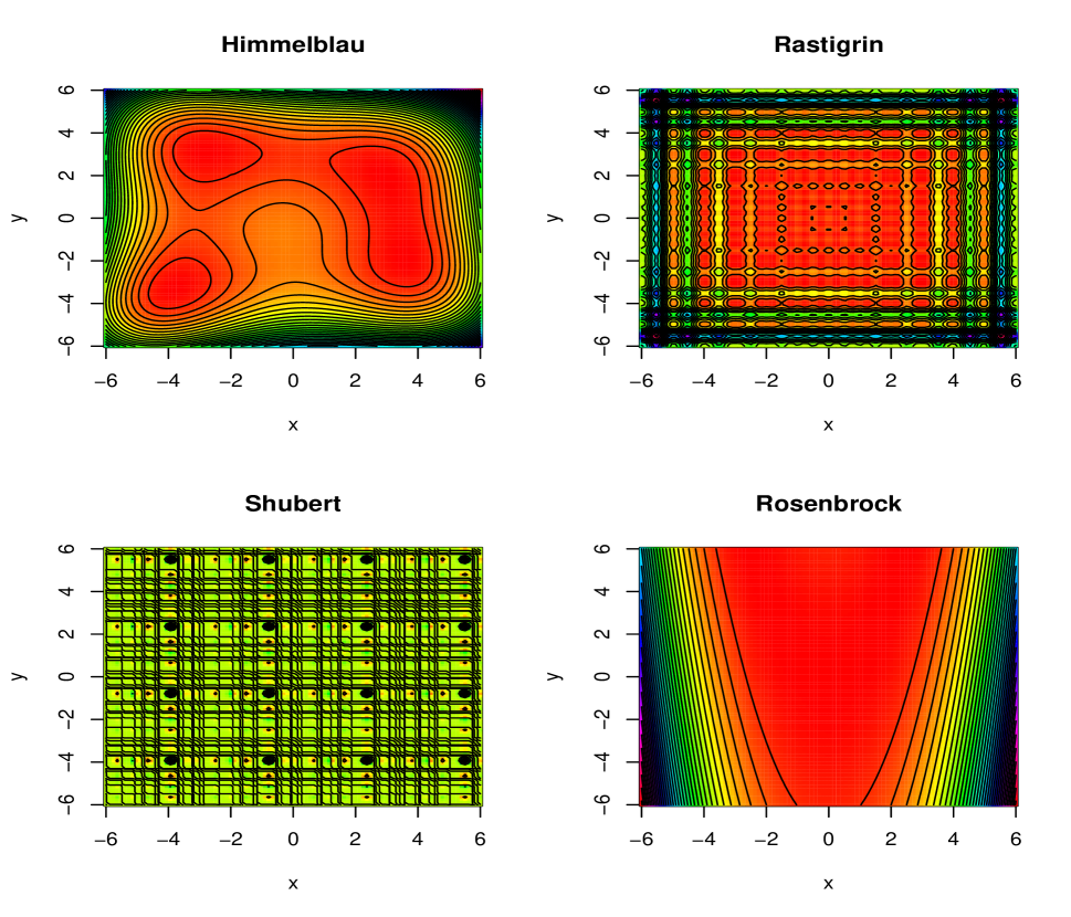
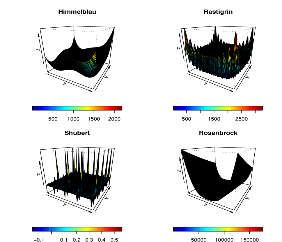
Figures 1 and 2 show contour and drape-plots of the Rosenbrock, Himmelblau, Rastigrin and Shubert functions. This set of functions exhibits a variety of challenges: a global mode in a long valley (Rosenbrock), multiple local and one global mode (Rastrigin) to multi-modality (Himmelblau, Shubert). For example, traditional derivative-based methods have difficulties for the Rosenbrock function to traverse its long steep valley.

Let $f({\bf x})=\sum_{i=1}^{K}f_{i}(x_{1},x_{2})$ be a bivariate additive objective function defined over a bounded region for ${\bf x}=\{x_{1},x_{2}\}\in\Re^{2}$. We will apply the exponential slice sampler as the functions to the Boltzmann distribution

$$\pi_{K}(x_{1},x_{2})=\exp\left(-\kappa\sum_{i=1}^{K}f_{i}(x_{1},x_{2})\right)/Z_{K}\;.$$

First, as in simulated tempering, we have to define a set of temperatures $\{\kappa_{1}<\ldots<\kappa_{m}\}$ to run our Markov chain. For all four examples, we pick $m=4$, and we use $\kappa\in\{0.1,0.5,1,5\}$ except for the Rosenbrock function where we set $\kappa\in\{1,5,50,5000\}$ which requires higher energy levels.

3.1 Rosenbrock function

Rosenbrock’s valley is a classic optimization problem that illustrates the difficulties with local search methods. The global minimum lays inside a long, narrow flat valley. Finding the valley is straightforward; however, getting to the minimum is hard. We need to find the minimum $(x_{1},x_{2})=(1,1)$ of the function:

$$f(x_{1},x_{2})=(1-x_{1})^{2}+c(x_{2}-x^{2}_{1})^{2}\;\;{\rm where}\;c=100\;.$$

The Boltzmann distribution has density

$$\pi_{K}(x_{1},x_{2})=\exp\left(-\kappa\left\{(1-x_{1})^{2}+c(x_{2}-x^{2}_{1})^{2}\right\}\right)/Z_{\kappa}\;.$$

There are a number of ways of introducing slice variables. We choose to slice out the last nonlinear factor. Let $(u|x_{1},x_{2})\sim Uni\left(0,\exp\left\{-\kappa c(x_{2}-x^{2}_{1})^{2}\right\}\right)$. Then we have a three variable joint distribution:

$$\pi_{\kappa}(x,y,u)=\exp\left\{-\kappa(1-x_{1})^{2}\right\}\mathbb{I}\left(0\leq u\leq\exp\left\{-\kappa c(x_{2}-x^{2}_{1})^{2}\right\}\right)/Z_{\kappa}.$$

We can implement MCMC using a partially collapsed Gibbs sampler (van Dyk and Park, 2008, Park and van Dyk, 2009). That is, we can marginalise $u$ out of the draw for $x_{2}$ and use the conditional $\pi(x_{2}|x_{1})$ rather than $\pi(x_{2}|x_{1},u)$. The complete conditionals are then:

$$\pi(x_{2}|x_{1}) \sim\mathcal{N}(x^{2}_{1},2/\kappa c),$$

$$\pi(x_{1}|x_{2},u) \sim\mathcal{N}(1,2/\kappa)\mathbb{I}\left(a(u,x_{2})\leq x\leq b(u,x_{2})\right),$$

$$\pi(u|x_{1},x_{2}) \sim Uni\left(0,\exp\left\{-\kappa c(x_{2}-x^{2}_{1})^{2}\right\}\right).$$

The interval $(a(u,x_{2}),b(u,x_{2}))$ is found by inverting the slice region:

$$u\leq\exp\left\{-\kappa c(x_{2}-x^{2}_{1})^{2}\right\}\;{\rm implies}\;x_{2}-\sqrt{-\ln u/\kappa c}\leq x^{2}_{1}\leq x_{2}+\sqrt{-\ln u/\kappa c}.$$

For $b>0$ and $a\leq x^{2}_{1}\leq b$, we have $-\sqrt{a}\leq x_{1}\leq\sqrt{b}$ and so

$$a(u,x_{2})=-\sqrt{x_{2}-\sqrt{-\ln u/\kappa c}}\;{\rm and}\;b(u,x_{2})=\sqrt{x_{2}+\sqrt{-\ln u/\kappa c}}.$$

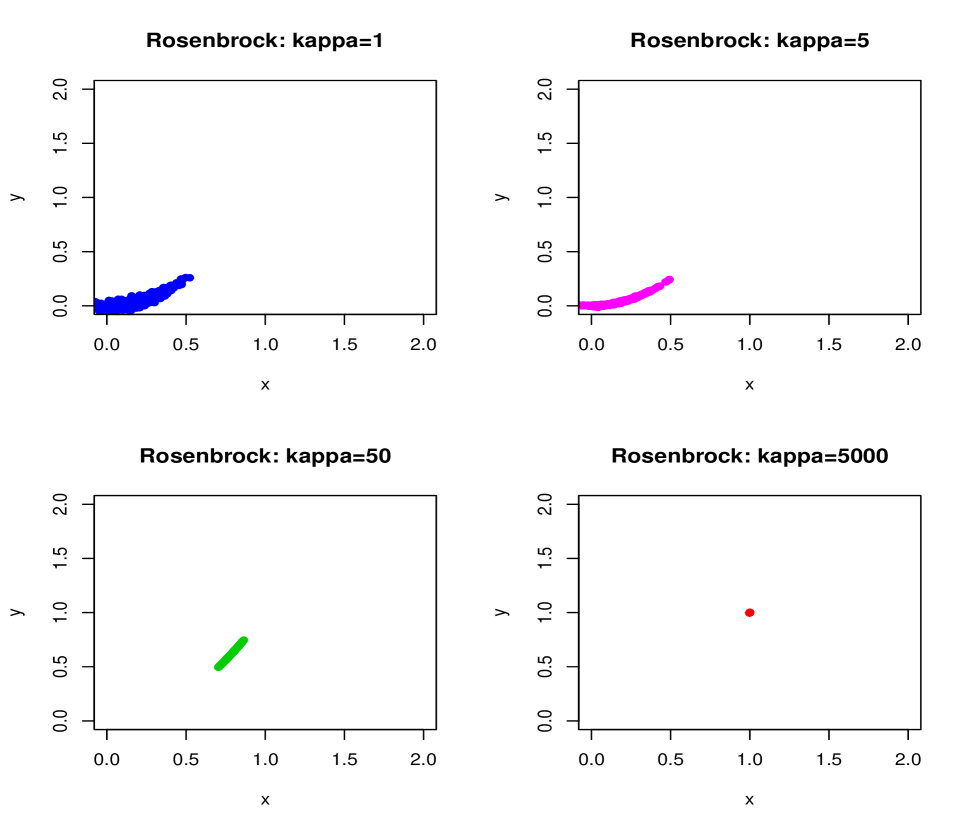
Figure 3 shows a sensitivity analysis for a range of energy values $\kappa\in\{1,5,50,5000\}$. We run our MCMC algorithm for $G=1000$ with a burn-in of $G_{0}=100$. Higher energy levels are required for the chain to travel along the valley to the minimum at $(x_{1},x_{2})=(1,1)$. As we increase $\kappa$, the slice sampler is able to traverse the valley and find the minimum.

3.2 Himmelblau’s function

Himmelblau’s function is defined by

$$f(x_{1},x_{2})=(x^{2}_{1}+x_{2}-11)^{2}+(x_{1}+x_{2}^{2}-5)^{2}.$$

This function has four identical local minima at zero and a local maximum at $(x_{1},x_{2})=(-0.27,-0.92)$. The minima are at

$$(3,2),(-2.805,3.131),(-3.779,-3.282),(3.584,-1.848)$$

with a function value of zero. The associated Boltzmann distribution is

$$\pi_{\kappa}(x_{1},x_{2})=\exp\left\{-\kappa\left((x^{2}_{1}+x_{2}-11)^{2}+(x_{1}+x_{2}^{2}-5)^{2}\right)\right\}/Z_{\kappa}\;.$$

Due to the quadratic terms also containing squares this distribution is not straightforward to simulate from. We observe that the following inequalities hold for the minima: $x_{1}^{2}+x_{2}-11<0$ and $x_{1}+x_{2}^{2}-5>0$.

To implement slice sampling, we use a latent variable augmentation $u=(u_{1},u_{2})$ and a joint distribution

$$\pi_{\kappa}(x_{1},x_{2},u_{1},u_{2})=\mathbb{I}\left(0\leq u_{1}\leq\exp\left\{-\kappa(x^{2}_{1}+x_{2}-11)^{2}\right\}\right)\mathbb{I}\left(0\leq u_{2}\leq\exp\left\{-\kappa(x_{1}+x_{2}^{2}-5)^{2}\right\}\right)/Z_{\kappa}\;.$$

Given $(u_{1},u_{2})$, we can invert the slice regions to obtain the inequalities:

$$-\kappa^{-1}\log u_{1}\geq(x^{2}_{1}+x_{2}-11)^{2}\;\;{\rm and}\;\;-\kappa^{-1}\log u_{2}\geq(x_{1}+x_{2}^{2}-5)^{2}.$$

Therefore, for $(x_{1}|x_{2})$, we have

$$a_{1}=11-x_{2}-\sqrt{-\kappa^{-1}\log u_{1}} \leq x^{2}_{1}\leq 11-x_{2}+\sqrt{-\kappa^{-1}\log u_{1}}=b_{1};$$

$$c_{1}=5-x_{2}^{2}-\sqrt{-\kappa^{-1}\log u_{2}} \leq x_{1}\leq 5-x_{2}^{2}+\sqrt{-\kappa^{-1}\log u_{2}}=d_{1}.$$

Given the inequalities: $a_{1}\leq x_{1}^{2}\leq b_{1}$ and $c_{1}\leq x_{1}\leq d_{1}$, we can first without loss of generality replace $a_{1}\rightarrow\max(a_{1},0)$ and assume that $a_{1}\geq 0$. Then, we have the union of the following regions:

$$-\sqrt{b_{1}}\leq x_{1}\leq-\sqrt{a_{1}}\;{\rm and}\;\sqrt{a_{1}}\leq x_{1}\leq b_{1}.$$

Combining, we have

$$\max\left(-\sqrt{b_{1}},c_{1}\right)\leq x_{1}\leq\min\left(-\sqrt{a_{1}},d_{1}\right)\;{\rm or}\;\max\left(\sqrt{a_{1}},c_{1}\right)\leq x_{1}\leq\min\left(\sqrt{b_{1}},d_{1}\right)$$

For the conditional $\pi(x_{2}|x_{1})$ we can argue in a similar fashion to obtain the constraints

$$a_{2}=5-x_{1}-\sqrt{-\kappa^{-1}\log u_{1}} \leq x_{2}^{2}\leq 5-x_{1}+\sqrt{-\kappa^{-1}\log u_{1}}=b_{2};$$

$$c_{2}=11-x_{1}^{2}-\sqrt{-\kappa^{-1}\log u_{2}} \leq x_{2}\leq 11-x_{1}^{2}+\sqrt{-\kappa^{-1}\log u_{2}}=d_{2}.$$

The complete set of conditionals is then given by:

$$\pi(x_{1}|x_{2},u_{1},u_{2}) \sim Uni\left(\max\left(-\sqrt{|a_{1}|},c_{1}\right),\min\left(\sqrt{b_{1}},d_{1}\right)\right),$$

$$\pi(x_{2}|x_{1},u_{1},u_{2}) \sim Uni\left(\max\left(-\sqrt{|a_{2}|},c_{2}\right),\min\left(\sqrt{b_{2}},d_{2}\right)\right),$$

$$\pi(u_{1}|x_{1},x_{2}) \sim Uni\left(0,\exp\left\{-\kappa(x^{2}_{1}+x_{2}-11)^{2}\right\}\right),$$

$$\pi(u_{2}|x_{1},x_{2}) \sim Uni\left(0,\exp\left\{-\kappa(x_{1}+x_{2}^{2}-5)^{2}\right\}\right).$$

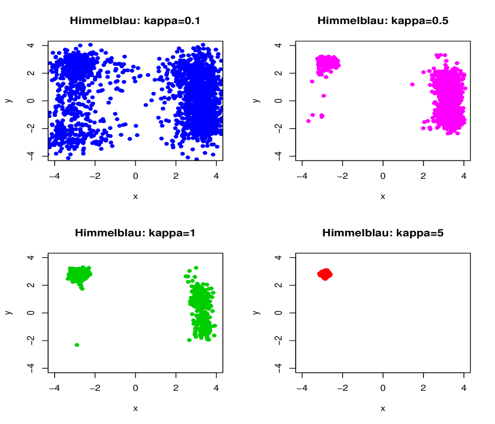
Figure 4 shows a sensitivity analysis to $\kappa\in\{0.1,0.5,1,5\}$. The slice sampler is again run for only $G=1000$ iterations with a burn-in of $G_{0}=100$. With longer chains and larger energy levels the algorithm will traverse the four modes with equal probability. Of the examples that we consider here, the Himmleblau function would benefit the most from a mixture energy level distribution to traverse the contours of the underlying function.

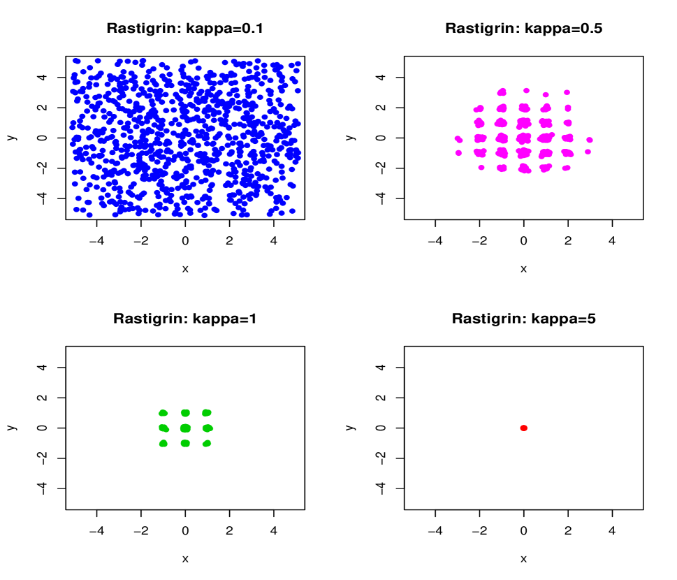
3.3 Rastrigin

The $2$-dimensional Rastrigin function is defined on the region $-5.12<x_{j}<5.12$ by:

$$f(x_{1},x_{2})=2A+\sum_{j=1}^{2}\left(x_{j}^{2}-A\cos(2\pi x_{j})\right)\;\;{\rm with}\;\;A=10$$

with a global minimum at $(x_{1},x_{2})=(0,0)$. The Boltzmann distribution then becomes

$$\pi_{\kappa}(x_{1},x_{2})=\exp\left\{-\kappa\sum_{j=1}^{2}x_{j}^{2}\right\}\exp\left\{\kappa A\sum_{j=1}^{2}\cos(2\pi x_{j})\right\}/Z_{\kappa}\;.$$

We use exponential slice variables $(y_{1},y_{2})$ and a joint distribution defined by

$$\pi_{\kappa}(x_{1},x_{2},y_{1},y_{2})=\exp\left\{-\kappa\sum_{j=1}^{2}x_{j}^{2}\right\}\mathbb{I}\left(-\kappa A\cos(2\pi x_{j})\leq y_{j}\right)e^{-y_{j}}/Z_{\kappa}\;.$$

The slice region is invertible and is specified by the set of inequalities for $j=1,2$

$$\cos(2\pi x_{j})\geq\left(-y_{j}/A\kappa\right)\;.$$

The conditional $x_{j}$ draw then results from a normal draw restricted to this interval set. A Gibbs sampler with the conditionals for $j=1,2$ is as follows:

$$\pi_{\kappa}(x_{j}|x_{-j},y) \sim\mathcal{N}\left(0,(2\kappa)^{-1}\right)\mathbb{I}\left(\cos(2\pi x_{j})\geq\left(-y_{j}/A\kappa\right)\right)$$

$$\pi_{\kappa}(y_{j}|x_{j}) \sim Exp[-\kappa A\cos(2\pi x_{j}),\infty)$$

For the implementation over $x_{j}\in[-5.12,5.12]$, we draw the truncated normals and truncated exponentials for the slice variables.

Figure 5 shows a sensitivity analysis to $\kappa\in\{0.1,0.5,1,5\}$ with $G=1000$ and a burn-in of $G_{0}=100$. Again slice sampling of the Boltzmann distribution finds the mode in a straightforward manner.

3.4 Shubert function

The Shubert function is defined within the domain $\mathbb{I}(-10,10)$ by

$$f(x_{1},x_{2})=-C(x_{1})C(x_{2})\;\;{\rm where}\;\;C(x)=\sum_{j=1}^{5}j\cos\left((j+1)x+j\right)\;.$$

We need to simulate from the Boltzmann distribution

$$\pi_{\kappa}(x_{1},x_{2})=e^{-\kappa\sum_{j=1}^{5}j\cos\left((j+1)x_{1}+j\right)\cdot\sum_{j=1}^{5}j\cos\left((j+1)x_{2}+j\right)}/Z_{\kappa}$$

For the conditional $\pi_{\kappa}(x_{1}|x_{2})$, we can write

$$\pi_{\kappa}(x_{1}|x_{2})=\prod_{j=1}^{5}e^{\kappa C(x_{2})j\cos\left((j+1)x_{1}+j\right)}.$$

We introduce a set of auxiliary slice variables $y_{j},1\leq j\leq 5$ for each $x_{i},i=1,2$ that are conditional exponentials. The corresponding joint is:

$$\pi_{\kappa}(x_{1},x_{2},y_{1},\ldots,y_{5})=\prod_{j=1}^{5}\exp(-\kappa y_{j})\mathbb{I}\left(y_{j}\geq C(x_{2})j\cos\left((j+1)x_{1}+j\right))\right)/Z_{\kappa}$$

This is inverted using the condition:

$$\left(\frac{y_{j}}{jC(x_{2})}\right)\mathbb{I}_{C(x_{2})<0}\leq\cos((j+1)x_{i}+j)\leq\left(\frac{y_{j}}{jC(x_{2})}\right)\mathbb{I}_{C(x_{2})>0}\;.$$

This gives a collection of intervals $I_{1}(y_{j},x_{2})$ for $1\leq j\leq 5$ for each of the slice variables; $x_{1}$ is then uniformly distributed over the intersection of these intervals, $\cap_{j}I_{1}(u_{j},x_{2})$.

Hence we can then run a Gibbs sampler with the conditionals, for $1\leq j\leq 5$:

$$\pi_{\kappa}(x_{1}|x_{2},y) \sim Uni(\cap_{j=1}^{5}I_{1}(y_{j},x_{2})),$$

$$\pi_{\kappa}(y_{j}|x_{1}) \sim Exp\left[C(x_{2})j\cos\left((j+1)x_{1}+j\right),\infty\right).$$

Similarly, this process is repeated for $\pi_{\kappa}(x_{2}|x_{1})$. This defines a $12$-dimensional Gibbs sampler that is able to traverse the joint distribution.

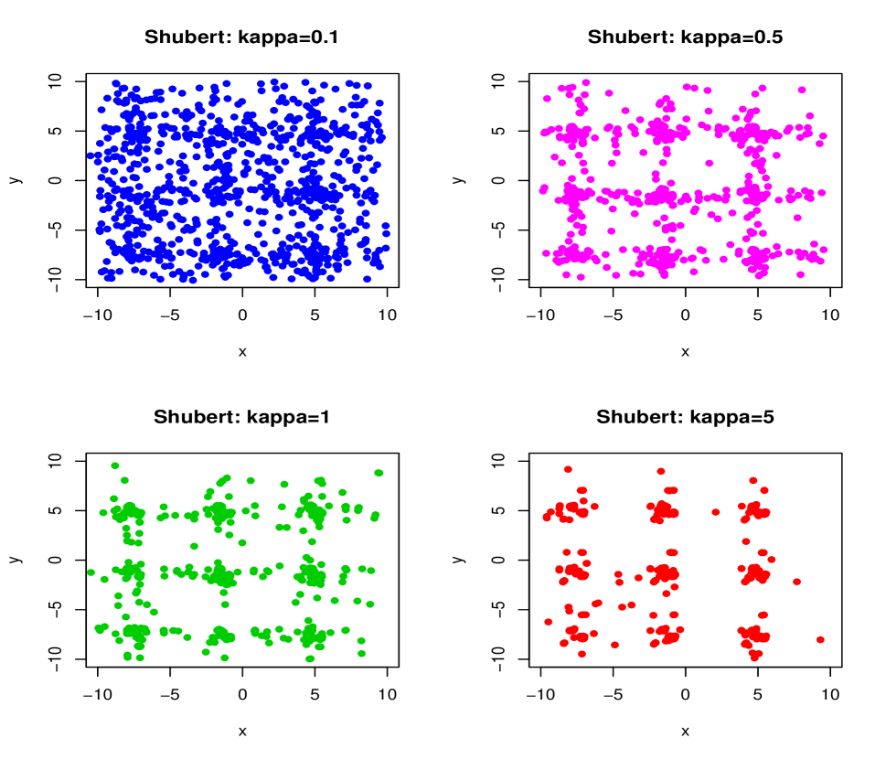
Figure 6 shows a sensitivity analysis to the same set of energy levels used for the Rastgrin and Himmleblau functions, namely $\kappa\in\{0.1,0.5,1,5\}$. Again the projected draws from the uniform slice region traverse the modes of the associated Boltzmann distribution in an efficient manner.

4 Discussion

We have described how slice sampling methods can be applied to functional optimisation. Our approach is parallelisable as in slice sampling (Tibbits et al, 2011). While we have only considered four test functions our methodology applies to a multitude of multi-modal functions, see Molga and Smutnicki (2005) for a list of possible candidates. Our approach is flexible enough to handle additive functions that are multiplicative. For example, the Michalewicz function is defined by $f(x_{1},x_{2})=-\sum_{i=1}^{2}sin(x_{i})sin^{2m}\left(ix_{i}^{2}/\pi\right)$ with $m=10$ (see Yang, 2010a,b). This function has a minimum of $-1.801$ at the point $(x_{1},x_{2})=(2.20319,1.57049)$ and it is challenge to fix the minimum. We also note that certain functions are straightforward as the Boltzmann distribution is conditionally normal. For example, the Booth function defined by $f(x_{1},x_{2})=(x_{1}+2x_{2}-7)^{2}+(2x_{1}+x_{2}-5)^{2}$ has a minimum of zero at the point $(x_{1},x_{2})=(1,3)$. The minimum can be identified without resorting to simulation as the Booth function can be factorised into the quadratic form $({\bf x}-\mu)^{\prime}Q^{-1}({\bf x}-\mu)$ where $x=(x_{1},x_{2})$ with $\mu=(1,3)$ and $Q=\frac{1}{9}\left(5,4;-4,5\right)$. Therefore, the minimum can be immediately identified without resorting to simulation.

There are clearly many other applications of these methods. For example, simulated annealing methods have been proposed in mixed integer non-linear programming problems (Cardoso et al, 1997) and in constrained optimisation (Geman and Geman, 1985, Geman, 1990, Whittle, 1992, Birge and Louveaux, 1997, Mueller, 2000, Asmussen and Glynn, 2008). Slice sampling the Boltzmann distribution provides a flexible alternative.

5 References

Aarts, E and Korst, J. (1989). Simulated Annealing and Boltzmann Machines. Wiley, NY.

Atchade, Y. and J. Liu (2010). The Wang-Landau algorithm in general state spaces: applications and convergence analysis. Statistica Sinica, 20, 209-233.

Asmussen, S. and P. Glynn (2008). Stochastic Simulation. Springer-Verlag, New York.

Azencott, R. (1988). Simulated Annealing. Seminaire Bourbaki, 697.

Berg, B.A. and T. Neuhaus (1992). Multicanonical ensemble: A new approach to simulate first-order phase transitions. Physical Review Letters, 68, 9-12.

Birge, J.R. and F. Louveaux (1997). Introduction to Stochastic Programming. Springer, New York.

Cardoso, M.F., R.L. Salcedo, S. Feyo de Azevedo and D. Barbosa (1997). A simulated annealing approach to the solution of mnlp problems. Computers Chem. Engng, 21(12), 1349-1384.

Devroye, L. (1986). Non-Uniform Random Variate Generation, Springer Verlag, New York.

Edwards, R.G. and A.D. Sokal (1988). Generalisation of the Fortuin-Kastelyn-Swendsen-Wang algorithm. Phys. Review D, 38(6), 2009-2012.

Geman, D. (1990). Random Fields and Inverse Problems in Imaging. Lecture Notes, Springer-Verlag, 113-193.

Geman, D. and S. Geman (1985). Relaxation and annealing with constraints. Technical Report 35, Brown University.

Geyer, C.J. (1992). Practical Markov chain Monte Carlo (with discussion). Statistical Science, 7, 473-511.

Geyer, C.J. and E.A. Thompson (1995). Annealing MCMC with applications to Ancestral Inference. Journal of the American Statistical Association, 90, 909-920.

Gidas, B. (1985). Nonstationary Markov chains and convergence of the annealing algorithm. J. Stat. Phys., 39, 73-131.

Gramacy, R.B. and H. Lee (2011). Optimisation under unknown constraints. Bayesian Statistics, 9, 229-257.

Gramacy, R. and M. Taddy (2010). Categorical Inputs, Sensitivity Analysis, Optimization and Importance Tempering in tgp. J. Statistical Software, 22(6), 1-48.

Janson, S. and M. Middendorf (2005). A Hierarchical Particle Swarm Optimiser and its Adaptive Variant. IEEE Trans in Systems, Man, and Cybernetics, 35(6), 1272-1282.

Kennedy, J. and R. Eberhart (1995). Particle Swarm Optimisation. IEEE Int. Conf. on Neural Networks, 1942-1948.

Kirkpatrick, S., C.D. Gelatt and M.P. Vecchi, (1983). Optimization by simulated annealing, Science, 220, 671-680.

Kou, S.C., Zhou, Q. and W.H. Wong (2006). Equi-Energy Sampler with applicationbs in statistical inference and statistical mechanics (with Discussion). Annals of Statistics, 34(4), 1581-1619.

Leman, S.C., Y. Chen and M. Lavine (2009). The Multi-Set Sampler. Journal of the American Statistical Association, 104, 1029-1041.

Liang, F. (2005). Generalized Wang-Landau algorithm for Monte Carlo computation. Journal of American Statistical Association, 100, 1311-1337.

Liang, F., C. Liu and R.J. Carroll (2007). Stochastic approximation in Monte Carlo computation. Journal of American Statistical Association, 102, 305-320.

Liu, J.S., Liang, F. and W.H. Wong (2000). The Multiple-Try Method and Local Optimisation in Metropolis Sampling. Journal of the American Statistical Association, 95, 121-134.

Liu, J.S., Liang, F. and W.H. Wong (2001). A theory of dynamic weighting in Monte Carlo. Journal of the American Statistical Association, 96, 561-573.

Marinari, E. and G. Parisi (1992). Simulated Tempering: A Monte Carlo scheme. Euro Phys. Lett. EPL, 19, 451-458.

Mira, A. and L. Tierney (2002). Efficiency and Convergence Properties of Slice Samplers. Scandinavian Journal of Statistics, 29(1), 1-12.

Molga, M. and C. Smutnicki (2005). Test functions for optimization needs. Working Paper.

Mueller, P. (2000). Simulation-Based Optimal Design. Bayesian Statistics, 6, 459-474.

Neal, R. (2003). Slice Sampling (with Discussion). Annals of Statistics, 31(3), 705-767.

Park, T. and D.A. van Dyk (2008). Partially Collapsed Gibbs Samplers: Theory and Methods. Journal of the American Statistical Association, 103, 790-796.

Pincus, M. (1968). A Closed Form Solution of Certain Dynamic Programming Problems. Operations Research, 16, 690-694.

Pincus, M. (1970). A Monte Carlo Method for Approximate Solution of certain types of Constrained Optimization Problems. Operations Research, 18(6), 1225-1228.

Polson, N.G. (1992). Comment on “Practical Markov chain Monte Carlo”. Statistical Science, 7, 490-491.

Polson, N. G. (1996). Convergence of Markov Chain Monte Carlo Algorithms. Bayesian Statistics 5, Bernardo et al eds, Oxford, 297-321.

Polson, N. G., J. G. Scott and J. Windle (2012). The Bayesian Bridge. Working Paper.

Roberts, G.O. and Polson, N. G. (1994). On the Geometric Convergence of the Gibbs Sampler. J. R. Statist. Soc., B, 56(2), 377-384.

Roberts, G.O. and J. Rosenthal (1999). Convergence of slice sampler Markov chains. J. R. Statist. Soc., B, 61, 643-660.

Taddy, M., H.K.H. Lee, G.A. Gray and J.D. Griffin (2009). Bayesian Guided Pattern Search for Robust Local Optimization. Technometrics, 51, 389-401.

Tibbits, M., M. Haran, J.C. Lietchy (2011). Parallel Multivariate Slice Sampling. Technical Report.

Tierney, L. (1994). Markov Chains for exploring Posterior Distributions (with discussion). Annals of Statistics, 22, 1701-1786.

Tweedie, R and K. Mengersen (1994). Rates of convergence of the Hastings-Metropolis algorithms. Annals of Statistics, 24, 101-121.

van Dyk, D.A. and T. Park (2009). Partially Collapsed Gibbs Samplers: Illustrations and Applications. Journal of Computational and Graphical Statistics, 18, 283-305.

Van Laarhoven P.J. and Aarts, E.H.J. (1987). Simulated Annealing: Theory and Applications, CWI Tract 51, Reidel, Amsterdam.

Wang, F. and D.P. Landau (2001). Efficient multi-range random walk algorithm to calculate the density of states. Phys. Rev. Lett, 86, 2050-2053.

Whittle, P. (1982). Optimization over Time (Volume 1). Wiley.

Yang, X-S (2010a). Test problems in Optimization. Working Paper, University of Cambridge.

Yang, X-S (2010b). Firefly algorithms for Multimodal Optimization. Working Paper, University of Cambridge.

Zhou, Q. and W.H. Wong (2008). Reconstructing the energy landscape of a distribution of Monte Carlo samples. Annals of Applied Statistics, 2(4),1307-1331.

Figure 1: Contour plots: Himmelblau, Rastigrin, Shubert and Rosenbrock

Figure 2: Drape plots: Himmelblau, Rastigrin, Shubert and Rosenbrock

Figure 3: Rosenbrock function: $f(x_{1},x_{2})=(1-x_{1})^{2}+100(x_{2}-x_{1}^{2})^{2}$. The minimum occurs at $(x_{1},x_{2})=(1,1)$.

Figure 4: Himmelblau function: $f(x_{1},x_{2})=(x_{1}^{2}+x_{2}-11)^{2}+(x_{1}+x_{2}^{2}-5)^{2}$. There are four idenital local minima at zero and a local maximum at $x_{1}=-0.27,x_{2}=-0.92$.

Figure 5: $2$-d Rastigrin function: $f(x_{1},x_{2})=2A+\sum_{j=1}^{2}(x_{j}^{2}-Acos(2\pi x_{j})$ with $A=10$ and $-5.12<x_{j}<5.12$.

Figure 6: Shubert function: $f(x_{1},x_{2})=-C(x_{1})C(x_{2})$ where $C(x)=\sum_{j=1}^{5}jcos\left((j+1)x+j\right)$.