Functional renormalization-group approach to decaying turbulence

Abstract

We reconsider the functional renormalization-group (FRG) approach to decaying Burgers turbulence, and extend it to decaying Navier-Stokes and Surface-Quasi-Geostrophic turbulence. The method is based on a renormalized small-time expansion, equivalent to a loop expansion, and naturally produces a dissipative anomaly and a cascade after a finite time. We explicitly calculate and analyze the one-loop FRG equations in the zero-viscosity limit as a function of the dimension. For Burgers they reproduce the FRG equation obtained in the context of random manifolds, extending previous results of one of us. Breakdown of energy conservation due to shocks and the appearance of a direct energy cascade corresponds to failure of dimensional reduction in the context of disordered systems. For Navier-Stokes in three dimensions, the velocity-velocity correlation function acquires a linear dependence on the distance, $\zeta_{2}=1$, in the inertial range, instead of Kolmogorov’s $\zeta_{2}=2/3$; however the possibility remains for corrections at two- or higher-loop order. In two dimensions, we obtain a numerical solution which conserves energy and exhibits an inverse cascade, with explicit analytical results both for large and small distances, in agreement with the scaling proposed by Batchelor. In large dimensions, the one-loop FRG equation for Navier-Stokes converges to that of Burgers.

1 Introduction

Describing Navier Stokes (NS) turbulence with the tools of statistical physics has remained a major challenge since Kolmogorov’s dimensional arguments leading to the $E(k)\sim\bar{\epsilon}^{2/3}k^{-5/3}$ energy spectrum for the 3D energy cascade [1, 2, 3, 4]. The simplest analytical method, Kraichnan’s direct interaction approximation closure scheme [5] (equivalent to mode coupling) failed to recover Kolmogorov’s prediction. There were numerous attempts to overcome these difficulties using a variety of methods, e.g. more refined closure schemes [6], large number of components [7, 8], renormalization-group (RG) [9, 10, 11, 12, 13, 14, 15] conjectures for short-distance expansions [16, 17, 18], study of short time singularities [19], tetrad models [20], and shell models [21], with various degrees of success. At the heart of the cascade phenomenon is that non smooth velocity field do not conserve energy. The main physics challenge, i.e. to describe the statistics of the energy transfer via singular or almost singular structures, is only partially captured. Predicting the multi-fractal corrections for velocity moments $S_{p}(u,t)=\langle\left[({\bf v}_{{\bf u}t}-{\bf v}_{0t})\cdot{\bf u}/|{\bf u}|\right]^{p}\rangle\simeq C_{p}|{\bf u}|^{\zeta_{p}}$ to Kolmogorov’s prediction ($\zeta^{\mathrm{K}}_{p}=p/3$) remains a challenge, despite the analytical progress in the simpler passive scalar problem [22, 23, 24, 25, 26, 27, 28, 29, 30, 31, 32, 33, 34, 35, 36, 37, 38, 39, 40]. For the inverse cascade in 2D [41], due to an infinity of conserved quantities, and a simpler numerical modeling, more is known; the most recent analysis unveils a tempting connection to conformal field theory and SLE [42], but remains based on numerics or speculative [43]. Also relations between Navier-Stokes and the membrane dynamics of black holes have been discussed in the context of the AdS/CFT correspondence [44, 45, 46] as well as relations to the physics of graphene [47].

The problem of $N$-dimensional Burgers turbulence, i.e. of a potential flow without pressure, exhibits similarities with Navier-Stokes turbulence, such as the existence of an inertial range which supports an energy cascade and the multi-scaling of the velocity moments. Although, as NS, it lacks a small control parameter and hence is non-trivial, it is simpler, since the Burgers equation can be integrated explicitly via the Cole-Hopf transformation , hence it has allowed for some progress [50, 48]. A remarkable mapping to an elastic object in a quenched random potential maps the shocks in both a decaying or stirred Burgers velocity field to the jumps of the equilibrium position of the pinned elastic object (which is a point for decaying Burgers or a line for stirred Burgers) upon variation of an external field. This mapping was used to study the large-dimension $N$ limit of stirred Burgers turbulence using replica symmetry breaking [51, 52] and, more recently, of decaying Burgers turbulence [53, 54]. The detailed statistics of shock cells which is obtained from these works is consistent with the physical expectation, and important open questions are now (i) whether this is a good starting point to perform an expansion towards finite $N$; (ii) whether it can inspire an approach to Navier Stokes in large dimension, a notably difficult problem [55]. An RG inspired method bypassing the Cole-Hopf transformation has been proposed very recently for the KPZ equation which is closely related to the Burgers equation [56].

Another powerful method able to handle singularities such as shocks and avalanches in disordered systems, which does not rely on large $N$, is the Functional Renormalization Group (FRG) [57, 58] (for an introduction and review see [59, 60]). The connection between the FRG and decaying Burgers turbulence was elucidated in [61, 62] (see [63] for an earlier attempt). It turns out that the force felt by an elastic manifold of internal dimension $d$ submitted to a random potential plus a quadratic well can be seen as a generalized velocity field: it satisfies an exact evolution equation which is a functional generalization of the decaying Burgers equation, where the role of time is played by the (inverse) curvature of the well. For $d=0$ the manifold is a point and one recovers the standard Cole-Hopf representation of the Burgers equation. The hierarchy of equations relating $n$-point equal-time velocity correlation functions identifies with the (exact) hierarchy of FRG flow equations, and the loop expansion in the field theory corresponds to the (renormalized) small time expansion in the (generalized) Burgers problem, as will be detailed below. The amazing property is that this hierarchy becomes controlled in an expansion in $\epsilon=4-d$ around $d=4$, which is the crucial property of the FRG approach to disordered systems. Hence Burgers turbulence, i.e. $d=0$, becomes accessible via this expansion. Furthermore the physics of the generalized Burgers problem (i.e. of the manifold) has features which are independent of the parameter $d$. For instance, energy conservation for smooth flows is obtained as well as an infinite number of conserved quantities (the first property being called ”dimension reduction” in the context of manifold, and the second corresponds to the non-renormalization of the moments of the so-called Larkin random force). Non-conservation of energy via shocks occurs for any $d$, and the dissipative anomaly at the heart of the energy cascade, i.e. the non-vanishing limit of the energy flux $-\partial_{t}{\cal E}=\bar{\epsilon}=\nu\langle(\nabla v)^{2}\rangle$ as $\nu\to 0$, is naturally captured by the FRG [61, 62]. Finally the FRG allows to compute shock-size distributions in the controlled expansion around $d=4$ [64, 65]. Most of these studies focused on $N=1$, but recently we also investigated $N>1$ [66].

The aim of this paper is thus to investigate whether FRG-inspired methods can be developed to describe Navier-Stokes turbulence as well. Here, our scope is relatively modest and it should be seen as a first exploration of the FRG method into the domain of non-linear physics. We focus on the decaying Burgers and Navier-Stokes equations; however, the stirred case can also be studied within the same framework. We derive the 1-loop FRG equations, first for Burgers in $N$-dimension (since most explicit calculations in [61, 62] were for $N=1$), and then for Navier-Stokes. We discuss some features of the fixed-point solutions which correspond to a decaying turbulent state, leaving a detailed analysis for the future. In $N=2$ we perform a detailed analysis of the NS fixed point. At this stage, the method for NS is not a controlled perturbative expansion scheme, since there is no equivalent of the Cole-Hopf mapping. The method however does capture some of the physics of the singularities. We analyze the nature of the singularities at small distance. While our analysis is restricted to one loop, we discuss at the end possible extensions to higher loops.

Let us stress that in the so-called inertial range of length and time scales, it is widely expected that the statistics of decaying turbulence is rather similar to the forced one. Indeed, due to strong separation of the large and small time scales, the eddies in the inertial range have enough time to reach an equilibrium for the energy-flux, before the larger eddies will significantly decay. The scaling behavior of decaying turbulence in the inertial range is thus indistinguishable from the forced case, while differences will occur at the scales of the large eddies. This is the universality assumption entering most theories of turbulence, see e.g. Ref. [67] for a detailed discussion.

The paper is organized as follows: In section 2, we introduce the model and notations. In section 3, we review known results, both for Burgers and Navier Stokes. The FRG equations are derived in section 4. We start by the general scheme, before giving results for Burgers and Navier Stokes; finally we discuss conserved quantities. In section 5, we discuss the short-distance singularity of the FRG equations: Are there solutions with other power laws than a cusp? In section 6 we focus on the analysis of the FRG equations for Navier-Stokes turbulence in two dimensions. In section 7 we discuss the limit of large $N$ and in section 8 we give the FRG equations for surface quasi geostrophic turbulence.

Finally note that this work was started a while ago. For an early exposition see [68].

2 Model and notations

We study here two models:

(i) the $N$-dimensional decaying Burgers equation for a $N$-component velocity field ${\bf v}_{{\bf u}t}$ at point ${\bf u}$ and time $t$,

$$\partial_{t}{\bf v}^{\alpha}_{{\bf u}t}=\nu\nabla_{{\bf u}}^{2}{\bf v}^{\alpha}_{{\bf u}t}-\frac{1}{2}\partial_{{\bf u}}^{\alpha}({\bf v}_{{\bf u}t})^{2}\ .$$ (1)

The velocity is assumed to be vorticity-free so it can be expressed as gradient of a potential function, ${\bf v}^{\alpha}_{{{\bf u}t}}=\partial^{\alpha}_{{\bf u}}\hat{V}({{\bf u},t})$, that implies $\frac{1}{2}\partial^{\alpha}({\bf v})^{2}=({\bf v}\cdot\nabla){\bf v}^{\alpha}$. Note that to streamline notations we attach space and time indices to the fields, which are never to be understood as derivatives. We use boldface to indicate vectors, and normal font for scalars, so $k:=|{\bf k}|$.

(ii) the incompressible $N$-dimensional Navier-Stokes equation

$$\partial_{t}{\bf v}^{\alpha}_{{\bf u}t}=\nu\nabla_{{\bf u}}^{2}{\bf v}^{\alpha}_{{\bf u}t}-P^{\rm T}_{\alpha\beta}(\partial_{{\bf u}})\partial^{\gamma}_{{\bf u}}({\bf v}^{\gamma}_{{\bf u}t}{\bf v}^{\beta}_{{\bf u}t}),\ \ \ \ \ \ \ \ P^{\rm T}_{\alpha\beta}(\partial_{{\bf u}})=\delta^{\alpha\beta}-\frac{\partial^{\alpha}_{{\bf u}}\partial^{\beta}_{{\bf u}}}{\nabla^{2}}$$ (2)

with the pressure eliminated using the transverse projection operator $P^{\rm T}_{\alpha\beta}(\partial_{{\bf u}})$. The latter implies the divergence free constraint (incompressibility) $\nabla\cdot{\bf v}=0$ at all times. In Fourier space, both equations can be written as

$$\partial_{t}{\bf v}^{\alpha}_{{\bf k}t}=-\nu k^{2}{\bf v}^{\alpha}_{{\bf k}t}-\frac{1}{2}P_{\alpha;\beta\gamma}({\bf k})\sum_{{\bf p}+{\bf q}={\bf k}}{\bf v}^{\beta}_{{\bf q}t}{\bf v}^{\gamma}_{{\bf p}t}\ ,$$ (3)

with

$$P_{\alpha;\beta\gamma}({\bf k})=\left\{\begin{array}[]{ll}\displaystyle i{\bf k}^{\alpha}\delta_{\beta\gamma}&\mbox{(Burgers)},\\ \displaystyle i{\bf k}^{\beta}P^{\rm T}_{\alpha\gamma}({\bf k})+i{\bf k}^{\gamma}P^{\rm T}_{\alpha\beta}({\bf k})&\mbox{(Navier Stokes)}.\\ \end{array}\right.$$ (4)

The transverse and longitudinal projection operators written in Fourier space read

$$P^{\rm T}_{\alpha\beta}({\bf k})=\delta^{\alpha\beta}-\frac{{\bf k}^{\alpha}{\bf k}^{\beta}}{k^{2}},\ \ \ \ \ \ \ P^{\rm L}_{\alpha\beta}({\bf k})=\frac{{\bf k}^{\alpha}{\bf k}^{\beta}}{k^{2}}.$$ (5)

In both cases we are interested in the small-viscosity (large Reynolds number) limit $\nu\to 0$, in which case a broad inertial range develops. In that limit the Navier-Stokes equation formally becomes the Euler equation, and in both cases weak solutions exist [69, 70, 71] (for review see [72]).

We study homogeneous turbulence with random initial conditions, i.e. we chose an initial condition at time $t=0$ which is statistically translational invariant. Everywhere we denote $\langle\dots\rangle$ the average over initial conditions. We assume that the initial velocity field is Gaussian distributed and that its spectral support is around a characteristic wave number $k_{0}$. The averaged squared initial velocity is $\bar{v}_{0}=\langle{\bf v}_{00}^{2}\rangle^{1/2}$. The initial Reynolds number is $\mathcal{R}=\bar{v}_{0}/(\nu k_{0})$ which we assume to satisfy $\mathcal{R}\gg 1$. The initial range (where viscosity is subdominant), given by $k_{0}\ll k\ll\bar{v}_{0}/\nu$, has no particular structure, but will develop, as time increases, into a self-similar inertial range where the energy cascade (in three dimensions) will take place.

To stress the similarity with the FRG, we denote the equal-time velocity two-point function as

$$\langle{\bf v}^{\alpha}_{{\bf u}t}{\bf v}^{\beta}_{0t}\rangle=\Delta_{t,\alpha\beta}({{\bf u}})\quad,\quad\langle{\bf v}^{\alpha}_{{\bf k}t}{\bf v}^{\beta}_{{\bf k}^{\prime}t}\rangle=\delta_{{\bf k}-{\bf k}^{\prime}}\Delta_{t,\alpha\beta}({\bf k})\ .$$ (6)

We denote $\delta_{{\bf k}}:=(2\pi)^{N}\delta^{N}({\bf k})$, and in Fourier space $\Delta_{t,\alpha\beta}({\bf k})=P^{\rm L,T}_{\alpha\beta}({\bf k})\Delta_{t}({\bf k})$ for Burgers and Navier-Stokes respectively. By definition, $\Delta_{\alpha\beta}({{\bf u}})=\Delta_{\beta\alpha}(-{{\bf u}})$, while symmetry is only assured for isotropic turbulence. We study a system in a periodic cube (torus) of volume $L^{N}$ with mostly two distinct cases:

(A) fixed $t$ and $L\to\infty$ in which case we further restrict to isotropic (homogeneous) turbulence where $\Delta_{t}({\bf k})$ depends only on $|{\bf k}|$.

(B) fixed $L$, which becomes periodic turbulence. In case (B) we use discrete Fourier modes $\sum_{\bf q}$, which implicitly become $\sum_{\bf q}\to\int_{\bf q}\equiv\int\frac{\rmd^{N}{\bf q}}{(2\pi)^{N}}$ in all formula below in case (A).

The total kinetic energy per unit volume, and the kinetic-energy spectrum are denoted as in [6]

$${\cal E}(t)=\frac{1}{2}\langle{\bf v}^{2}\rangle=\int_{0}^{\infty}\rmd k\,{\cal E}(k,t)\ .$$ (7)

However for convenience we also use a non-standard normalization for energy and energy spectrum and denote ($S_{N}$ is the area of the unit sphere in dimension $N$):

$$E(t):=\frac{(2\pi)^{N}}{S_{N}}\langle{\bf v}^{2}\rangle=\int_{0}^{\infty}\rmd k\,E(k,t)\ ,$$ (8)

$$E(k,t):=\int\frac{\rmd^{N}{\bf k}}{S_{N}}\delta(k-|{\bf k}|)\Delta_{t,\alpha\alpha}({\bf k})\ ,$$ (9)

which for isotropic turbulence becomes

$$E(k,t)=k^{N-1}\Delta_{t,\alpha\alpha}(k)\ .$$ (10)

Hence ${\cal E}(k,t)=\frac{1}{2}\frac{S_{N}}{(2\pi)^{N}}E(k,t)$. The decay of turbulence depends on the initial spatial behavior of the energy spectrum at large scales, hence we denote (in the isotropic case)

$$E(k,t=0)\sim_{k\to 0}c\,k^{n}\ ,\ \quad\Delta_{0,\alpha\alpha}({\bf k})\sim_{k\to 0}c\,k^{n-N+1}\ ,\ \quad\Delta_{0,\alpha\alpha}({\bf u})\sim_{u\to\infty}c^{\prime}u^{-n-1}\ .$$ (11)

The total (kinetic) energy (per unit volume) $E(t)=\int_{0}^{\infty}\rmd k\,E(k,t)\sim\Delta_{t,\alpha\alpha}({\bf u}=0)$ must be finite (it grows as $L^{n+1}$ for $n<-1$) and the initial velocity field is usually assumed to be smooth, i.e.  $\Delta_{0,\alpha\beta}({{\bf u}})$ is an analytic function in each of its components ${\bf u}$ near $|{\bf u}|=0$.

In all cases below, when the system reaches a statistically scale invariant decaying state, we denote by

$${\ell}(t)=t^{\zeta/2}$$ (12)

the characteristic length scale, which usually separates the inertial range from the large-scale region (i.e. $\ell(t=0)\sim 1/k_{0}$). The notation is motivated by the relation, in the Burgers case, to the roughness exponent $\zeta$ for random manifolds. We distinguish it from the exponent $\zeta_{2}$, which describes the leading short-distance singular behavior of the two-point equal-time velocity correlator in the inviscid limit. We will also assume a dissipation scale $\ell_{d}(t)\ll\ell(t)$ which is the lower boundary of the inertial range, and is often set to zero in the following, corresponding to the inviscid limit.

3 Known results and phenomenology

3.1 Decaying Burgers

In the following we use the mapping of the Burgers equation onto the problem of a particle in the $N$-dimensional potential $W=V({\bf u}_{0})+\frac{1}{2t}({\bf u}-{\bf u}_{0})^{2}$, where $V({{\bf u}})$ is the random potential which parameterizes the initial condition, i.e. ${\bf v}_{{\bf u}t=0}=\nabla_{{\bf u}}V({\bf u})$. Denoting by $Z$ the canonical partition function of the particle at temperature $T=2\nu$, the velocity at all times is ${\bf v}_{{\bf u}t}=\nabla_{{\bf u}}\hat{V}({\bf u},t)$, where $\hat{V}({\bf u},t)=-T\ln Z$ is the free energy. In the inviscid limit it becomes $\hat{V}({\bf u},t)=\min_{{\bf u}_{0}}W$. Let us summarize what is expected for Burgers (most results are shown for $N=1$, and conjectured for $N>1$), for more details see e.g. [48] and the discussion in Section E of [62] including connections to the FRG. We assume a smooth Gaussian initial velocity field with the correlator (11), i.e., with a spectrum proportional to $|k|^{n}$ at small $k$ and decreasing quickly at large $k$. For isotropic turbulence (A) there are two cases:

(1) Long-range initial condition (LR) $n<1$: The correlator of the random potential $\langle[V({{\bf u}})-V(0)]^{2}\rangle$ grows as $u^{1-n}$ at large $u$ and the particle is always in a glass phase, i.e.  the effective viscosity scales to zero (see below). The evolution is expected to reach an asymptotic statistically scale invariant form ${\bf v}_{{\bf u}t}=\ell(t)t^{-1}\tilde{\bf v}(u/\ell(t))$ (in law) with $\ell(t)=t^{\zeta/2}$, where $\zeta=4/(3+n)$ and with energy decay $E(t)\sim t^{-2+\zeta}=t^{-2(n+1)/(n+3)}$. Shocks, i.e.  codimension-one manifolds (together with some additional lower dimensional singularities for $N>1$), where the velocity is discontinuous (at $\nu=0^{+}$) or nearly discontinuous (at small $\nu>0$), form in finite time and, convected by the flow, keep merging when they meet. The growing scale of this coarsening process (quite complicated for $N>1$) is expected to scale as $\ell(t)\sim t^{\zeta/2}$. This is clear at least for $N=1$ . While the width of an isolated shock grows as $L_{d}(t)\sim\nu t$, the width of the surviving shocks grows as $L^{\prime}_{d}(t)\sim\nu t^{1-\zeta/2}$ [61, 62], hence the rescaled width $L^{\prime}_{d}(t)/\ell(t)\sim\nu t^{1-\zeta}\equiv\nu_{\rm eff}$ scales to zero for $n<1$. This corresponds in the FRG to an attractive zero-viscosity (i.e. zero-temperature) fixed point (describing a glass phase for the particle): One can write $\nu_{\rm eff}=\nu t^{\theta/2}$, i.e.  $T_{\rm eff}=Tt^{\theta/2}$. For a random manifold, the glass exponent is $\theta=d-2+2\zeta>0$, with here $d=0$. This is a LR fixed point, with exponents given by their dimensional values (also called Flory values in the context of elastic manifolds), i.e.  they are fixed by the initial condition. This property, called the persistence of large eddies in turbulence, means that the energy spectrum for $k\ll 1/\ell(t)$ retains its original form (11) with an amplitude $c$ independent of time.

(2) Short-range initial condition (SR) $n>n_{c}=1$: This is the Kida regime [48, 73] with an asymptotic statistically scale invariant form (see however below) with a scale $\ell(t)=[t/(\ln t)]^{1/2}$ and a decay of the energy $E(t)\sim 1/[t(\ln t)^{1/2}]$ (for gaussian initial conditions). The (rescaled) shock width now grows (there is no glass phase); hence it exists only for $\nu\to 0$ before $t\to\infty$ (see [74, 75] for a more refined analysis of the double limit).

There is an additional crossover region (e.g. for $1<n<2$ for $N=1$) where the persistence of large eddies (i.e.  of the tail of the FRG function) still holds, but the system flows to the SR (Kida) fixed point: This is known as the Gurbatov phenomenon [76], i.e.  the velocity statistics is not scale invariant. The resulting energy spectrum then consists of three regions: (i) the “outer region”, $0<k<k_{s}(t)\sim t^{-1/[2(2-n)]}$, where the velocity correlations preserve its initial form (11); (ii) the “inner region”, $k_{s}(t)<k<{\ell(t)}^{-1}\sim t^{-1/2}$ ($\zeta=1$), with spectrum $k^{2}$, and (iii) the shock-dominated region with spectrum $k^{-2}$ for $k>{\ell(t)}^{-1}$. All scales are given up to logarithmic corrections and for $N=1$. More details can be found in [76]. Within the FRG analysis, this crossover region can be seen as crossover from the LR to the SR FRG fixed point. In the FRG analysis of random manifolds a similar crossover was described in [77].

In the marginal case $n=1,$ a LR fixed point exists where the potential retains logarithmic correlations, with a phase transition as a function of $\nu$ [75].

Note that originally Burgers [78] distinguished only two cases (for $N=1$), assuming that $J=\Delta(k=0)=\int\rmd u\Delta(u)$ exists. The case $J>0$ then corresponds to the LR case $n=0$, hence $\ell(t)\sim t^{2/3}$ ($\zeta=4/3$) and is usually called “random-field” fixed point in the language of random manifolds. The case $J=0$ was solved by Kida [73], and corresponds here to the SR case $n>1$ (for instance for $n=2$, $\Delta(k)$ is analytic and the random potential has $\delta$-correlations). This is usually called the “random-bond” fixed point in the language of random manifolds. The summary presented above contains many more cases, i.e. the LR models form a line of FPs, continuously parameterized by $n$, and the SR case can also be modified by the Gurbatov LR-SR crossover.

Finally for the periodic case, the system converges, for $N=1$, to a single random shock per period with $E(t)\sim t^{-2}$. This corresponds to the FRG random-periodic FP $\zeta=0$ (i.e.  $n=\infty$), and a similar picture should hold for any $N$.

3.2 Decaying Navier Stokes

A similar discussion can be given for decaying NS, though on a much less firm basis, mostly phenomenology, scaling arguments, closure calculations and some support from experiments. Again since Von Karman and Howarth [79] one assumes a decaying state ${\bf v}_{{\bf u}t}=\ell(t)t^{-1}\tilde{\bf v}({\bf u}/\ell(t))$ (in law). Then $\tilde{\bf v}$ satisfies a equation where $\nu\to\nu t/\ell(t)^{2}$, which flows to zero if $\zeta>1$. In Fourier this can be written ${\bf v}_{{\bf k}t}=\ell(t)^{2}t^{-1}\hat{\bf v}\big{(}{\bf k}\ell(t)\big{)}$ (in law) and the energy spectrum takes the form $E(k,t)=\ell(t)^{3}/t^{2}\tilde{E}\big{(}k\ell(t)\big{)}$ with $\ell(t)=t^{\zeta/2}$ and a total kinetic energy decay $E(t)\sim t^{-2+\zeta}$. The persistence of large eddies, i.e. the invariance of $E(k,t)\simeq ck^{n}$, implies $\zeta=4/(3+n)$. This corresponds to a LR initial condition (i.e. regime (1) in the previous section). The energy spectrum can then be divided into a low-wavenumber range $k\ell(t)\ll 1$ with $E(k,t)\simeq ck^{n}$, and the inertial range $k\ell(t)\gg 1$, with, in 3D ($N=3$), ${\cal E}(k,t)\simeq C_{K}\epsilon(t)^{2/3}k^{-5/3}$ (assuming Kolmogorov spectrum) with $d{\cal E}/dt=-\bar{\epsilon}(t)$. For more details see [6] VII-10, Ref. [80] for RG arguments, and [81].

There is agreement that this LR regime cannot hold for $n\geq 4$ because of the $C(t)k^{4}$ backtransfer in the energy spectrum discovered by Proudman and Reid [82] for the 3D Navier-Stokes equation, and found in EDQNM closure calculations [6] (analogous to the $k^{2}$ backtransfer for the Burgers dynamics). In other words, the low-$k$ energy spectrum cannot be softer than $k^{4}$. For $n>4$ it is argued that the small-$k$ part of the spectrum is replaced by $E(k,t)\sim C(t)k^{4}$ at small $k$, with the inertial range at large $k$. Because of the Gurbatov phenomenon (analogous to the situation in Burgers discussed above) it is then argued [83] that the LR regime cannot hold for $n<n_{c}$ with $3<n_{c}<4$. In the range $n_{c}<n<4$ there are three spectral regions $E(k,t)\simeq ck^{n}$ for $k<1/\ell_{*}(t)$ (outer region), $E(k,t)\simeq C(t)k^{4}$ for $1/\ell_{*}(t)<k<1/\ell(t)$ (inner region) and finally the inertial range for $k>1/\ell(t)$, leading to a breakdown of global self-similarity. This global picture seems compatible with experiments [84, 85].

Note that in 3D NS there is another conserved quantity, the helicity $h=\epsilon_{\alpha\beta\gamma}{\bf v}_{\alpha}\partial_{\beta}{\bf v}_{\gamma}$. It is locally fluctuating even if its average is zero. If its average is non-zero, as in MHD, then we need to consider $\Delta_{\alpha\beta}({{\bf u}})\neq\Delta_{\beta\alpha}({{\bf u}})=\Delta_{\alpha\beta}(-{{\bf u}})$. Its presence makes possible a joint cascade with two fluxes, one of energy and one of helicity, both to small length scales [86].

4 FRG equations

4.1 Loop expansion: General strategy

We now write FRG-like equations able to access directly the strong-coupling regime (i.e. finite non-linearity) using either a graphical method or, equivalently, starting from the exact infinite hierarchy obeyed by the equal-time $n$-point correlation functions denoted here $\langle{\bf v}^{\alpha_{1}}_{{\bf u}_{1}t}{\bf v}^{\alpha_{2}}_{{\bf u}_{2}t}...{\bf v}^{\alpha_{n}}_{{\bf u}_{n}t}\rangle=C^{(n)}_{\alpha_{1}...\alpha_{n}}({{\bf u}_{1},{\bf u}_{2},...,{\bf u}_{n}})$. They obey, for $n\geq 2$,

$$\partial_{t}C^{(n)}_{\alpha_{1}...\alpha_{n}}({{\bf u}_{1},{\bf u}_{2},...,{\bf u}_{n}}) = n\nu\;{\rm Sym}\left[\nabla_{{\bf u}_{1}}^{2}C^{(n)}_{\alpha_{1}...\alpha_{n}}({{\bf u}_{1},{\bf u}_{2},...,{\bf u}_{n}})\right]$$ (13)

$$-\frac{n}{2}\;{\rm Sym}\left[P_{\alpha_{1};\beta\gamma}(\nabla_{{\bf u}_{1}})C^{(n+1)}_{\beta\gamma\alpha_{2}...\alpha_{n}}({{\bf u}_{1},{\bf u}_{1},{\bf u}_{2},...,{\bf u}_{n}})\right]\ .$$

The time dependence is implicit, and $P_{\alpha;\beta\gamma}(\nabla)$ is given by Eqs. (4) and (5) rewritten in real space using $i\mathbf{k}\leftrightarrow\nabla$; symmetrization with respect to the $n$ pairs $({\bf u}_{i},\alpha_{i})$ for $i=1,...,n$ is denoted by ${\rm Sym}[...]$. We recall that $C^{(2)}_{\alpha_{1}\alpha_{2}}({{\bf u}_{1},{\bf u}_{2}})=\Delta_{t,\alpha_{1}\alpha_{2}}({\bf u}_{1}-{\bf u}_{2})$. In Fourier space the hierarchy reads

$$\partial_{t}C^{(n)}_{\alpha_{1}...\alpha_{n}}({{\bf k}_{1},{\bf k}_{2},...,{\bf k}_{n}}) = -n\nu\;{\rm Sym}\left[{\bf k}_{1}^{2}C^{(n)}_{\alpha_{1}...\alpha_{n}}({{\bf k}_{1},{\bf k}_{2},...,{\bf k}_{n}})\right]$$ (14)

$$-\frac{n}{2}\;{\rm Sym}\Big{[}P_{\alpha_{1};\beta\gamma}({\bf k}_{1})\sum_{{\bf p}+{\bf q}={\bf k}_{1}}C^{(n+1)}_{\beta\gamma\alpha_{2}...\alpha_{n}}({{\bf p},{\bf q},{\bf k}_{2},...,{\bf k}_{n}})\Big{]}$$

for the correlations $\langle{\bf v}^{\alpha_{1}}_{{\bf k}_{1}t}...{\bf v}^{\alpha_{n}}_{{\bf k}_{n}t}\rangle=C^{(n)}_{\alpha_{1}...\alpha_{n}}({\bf k}_{1},...,{\bf k}_{n})=\hat{C}^{(n)}_{\alpha_{1}...\alpha_{n}}({{\bf k}_{1},...,{\bf k}_{n}})\delta_{{\bf k}_{1}+...+{\bf k}_{n}}$, and we also define $\hat{C}^{\alpha_{1}\alpha_{2}}({\bf k},-{\bf k})=C^{\alpha_{1}\alpha_{2}}({\bf k})$.

If equation (13) is considered in the inertial range, i.e.  all $|{\bf u}_{ij}|\gg\ell_{d}$, it is expected (and for Burgers in some cases shown) that one can neglect the viscosity term in the hierarchy. To study the inertial range it is thus tempting to consider the limit $\nu=0^{+}$ of these equations. To argue that this can be done, and that the result is still given by equation (13) setting $\nu=0$, we need two conditions: (i) the physical requirement that the $n$-point velocity correlations $C^{(n)}$ are continuous functions, i.e. that limits at coinciding arguments exist; (ii) the property that the $\nu\to 0$ limit of averages such as $\langle\Phi({\bf u}_{i})P^{\rm T}_{\alpha\beta}(\partial_{{\bf u}})\partial^{\gamma}_{{\bf u}}({\bf v}^{\gamma}_{{\bf u}t}{\bf v}^{\beta}_{{\bf u}t})\rangle$ where $\Phi$ is any product of velocities with ${\bf u}_{i}\neq{\bf u}$ is equal to $P^{\rm T}_{\alpha\beta}(\partial_{{\bf u}})\partial^{\gamma}_{{\bf u}}\langle\Phi({\bf u}_{i}){\bf v}^{\gamma}_{{\bf u}t}{\bf v}^{\beta}_{{\bf u}t}\rangle$. This appears to be related to the existence of weak solutions of the Euler equation, which is discussed in [69, 70, 71, 72]. In some cases, e.g. for the inviscid Burgers equation and $N=1$, it can be justified [61, 62] from the dilute shock picture of [87].

Assuming that the $\nu=0$ hierarchy holds, let us describe the strategy of the loop expansion as it was constructed in the case of Burgers [61, 62]. It amounts to looking for a solution of the hierarchy in the schematic form (complicated convolutions are indicated by $*$):

$$\partial_{t}\Delta =t\Delta*\Delta+t^{3}\Delta*\Delta*\Delta+...$$ (15)

$$C^{(3)} =t\Delta*\Delta+t^{3}\Delta*\Delta*\Delta+...\quad,\quad C^{(4)}=\Delta*\Delta+t^{2}\Delta*\Delta*\Delta+...$$ (16)

$$C^{(5)} =t\Delta*\Delta*\Delta+...\quad,\quad\qquad\quad~{}~{}~{}\,C^{(6)}=\Delta*\Delta*\Delta+...\ .$$ (17)

It is illustrated here to two loops, and more generally $C^{(n)}=\sum_{q\geq 0}t^{2q+\epsilon_{q}}C^{(n)}_{q}[\Delta]$ with $\epsilon_{q}=0,1$ for $n\geq 3$ respectively even and odd. We impose that at $t=0$ the distribution is Gaussian, hence the functionals $C^{(2k)}_{0}[\Delta]$, $k\geq 1$, are given by the Wick decomposition. This allows to compute iteratively all the terms in the beta function (15): e.g. to one loop we start from $C^{4}_{0}=3[\Delta\Delta]$, and use (13) with successively $n=3$ and $n=2$, first to get $C^{3}_{0}$, then to get the one-loop $\Delta^{2}$ term in (15). Thus, the beta function appropriate to the rescaling $\Delta=t^{-2}\tilde{\Delta}$ is obtained directly. Counter-terms are produced automatically by successive corrections, due to consistent evaluations of $\partial_{t}\Delta$ terms at each step. Higher-loop calculations will be presented elsewhere [88]. The first corrections to each cumulant, i.e.  the $C^{(2k)}_{1}[\Delta]$ and $C^{(2k+1)}_{0}[\Delta]$ are the tree approximation. For calculations per se, an equivalent procedure, which we also performed to one loop using a graphical method directly on the Burgers and Navier-Stokes equations, is to compute $\Delta_{t}=\Delta_{t=0}+\sum_{q}t^{2q}\Delta_{t=0}^{*(q+1)}$ as a direct small-time expansion, then compute $\partial_{t}\Delta_{t}$ and re-express the result in terms of $\Delta_{t}$ itself as given in (15) by inverting the series. The information contained in the beta function can thus be described as a renormalized small-time expansion (for a direct small-time expansions see [55, 19]).

Note that the present FRG is different from the usual RG for turbulence as developed in [9, 10, 11, 12, 13, 14, 15]. Here we keep the complete crucial information about $\Delta(k)$ (in Fourier) while the usual RG integrates out shells in $k$. In particular, the information in the small-$u$ behavior of $\Delta({{\bf u}})\sim u^{\zeta_{2}}$ determines the exponent $\zeta_{2}$.

4.2 FRG equation for Burgers

We now display the resulting one-loop $\beta$-function for Burgers. Calculations in real space are given in A, and in Fourier space in B. A graphical derivation can be found in D. The result reads

$$\partial_{t}\Delta_{\alpha\beta}({{\bf u}})=-t\partial_{\alpha}\partial_{\beta}\Big{[}\Delta_{\gamma\delta}({{\bf u}})-\Delta_{\gamma\delta}(0)\Big{]}^{2}\ .$$ (18)

It has the usual form of the $N$-component one-loop FRG equation [77, 89]. To study the evolution from the initial condition (11), it is more convenient to introduce the rescaled velocity correlation $\tilde{\Delta}_{t,\alpha\beta}({{\bf u}})$ defined through

$$\Delta_{t,\alpha\beta}({{\bf u}})=\frac{1}{4}t^{\zeta-\frac{\epsilon}{2}}\tilde{\Delta}_{t,\alpha\beta}({\bf u}/t^{\zeta/2})\ .$$ (19)

everywhere in this section we introduce:

$$\epsilon=4$$ (20)

for Burgers, while $\epsilon=4-d$ for the manifold allows perturbative control. The rescaled velocity correlation satisfies

$$t\partial_{t}\tilde{\Delta}_{\alpha\beta}({{\bf u}})=\left(\frac{\epsilon}{2}-\zeta+\frac{\zeta}{2}{\bf u}\cdot\nabla_{{\bf u}}\right)\tilde{\Delta}_{\alpha\beta}({{\bf u}})-\frac{1}{4}\partial_{\alpha}\partial_{\beta}\Big{[}\tilde{\Delta}_{\gamma\delta}({{\bf u}})-\tilde{\Delta}_{\gamma\delta}(0)\Big{]}^{2}\ .$$ (21)

Using $\tilde{\Delta}_{\alpha\beta}({{\bf u}})=-\partial_{\alpha}\partial_{\beta}\tilde{R}({{\bf u}})=:-\tilde{R}^{\prime\prime}_{\alpha\beta}({{\bf u}})$, it can be recast as an equation for the correlator of the random potential of the particle problem

$$t\partial_{t}\tilde{R}({\bf u})=\left(\frac{\epsilon}{2}-2\zeta+\frac{\zeta}{2}{\bf u}\cdot\nabla_{{\bf u}}\right)\tilde{R}({\bf u})+\frac{1}{4}\left[\tilde{R}^{\prime\prime}_{\alpha\beta}({\bf u})^{2}-2\tilde{R}^{\prime\prime}_{\alpha\beta}(0)R^{\prime\prime}_{\alpha\beta}({\bf u})\right]\ .$$ (22)

One recovers the familiar zero-temperature FRG equation for manifolds, derived here directly for the inviscid Burgers problem in $N$ dimension, i.e. for $d=0$, by identifying $t\partial_{t}=-\frac{1}{2}m\partial_{m}$ (for $N=1$ it was obtained to 4 loops in [61, 62]).

Let us focus on isotropic turbulence and denote $R({\bf u})=h(u)$, the general case being very similar. The first property of the above FRG equations is that as long as the velocity flow is smooth, $\Delta_{\gamma\delta}({{\bf u}})-\Delta_{\gamma\delta}(0)\simeq-\frac{1}{3!}h^{\prime\prime\prime\prime}(0)(u^{2}\delta_{\gamma\delta}+2u_{\gamma}u_{\delta}),$ hence from equation (18) the energy is conserved,

$$\partial_{t}{\mathcal{E}}(t)={\frac{1}{2}}\partial_{t}\Delta_{\alpha\alpha}(0)=0\ ,$$ (23)

in agreement with standard knowledge for Burgers flows. However it is known (since Larkin, for review see e.g. [90] in the context of elastic manifolds) that $h^{\prime\prime\prime\prime}(0)$ diverges in a finite time $t_{c}$. Furthermore it is known since [57, 77, 91] that the solution of the one-loop equation $\Delta_{t,\alpha\beta}({{\bf u}})$ develops a cusp at the origin, more precisely $h(u)=h(0)+h^{\prime\prime}(0)\frac{u^{2}}{2}+h^{\prime\prime\prime}(0)\frac{u^{3}}{6}+...$, a property which was found to hold also to next order (two loop) [89] and, from the physics of shocks, is believed to hold to any order. Hence in the present context of Burgers turbulence it implies non-conservation, and decay, of the kinetic energy,

$$\partial_{t}{\mathcal{E}}(t)={\frac{1}{2}}\partial_{t}\Delta_{\alpha\alpha}(0)=-t\frac{N(N+3)}{4}h^{\prime\prime\prime}(0)^{2}\simeq-\frac{N(N+3)}{4^{3}}\tilde{h}^{\prime\prime\prime}(0)^{2}t^{\zeta-3},$$ (24)

using that now $\Delta_{\gamma\delta}({{\bf u}})-\Delta_{\gamma\delta}(0)\simeq-\frac{1}{2}h^{\prime\prime\prime}(0)u(\delta_{\gamma\delta}+\hat{u}_{\gamma}\hat{u}_{\delta})$ where in the last equation we have substituted the scaling form (19) valid at large $t$. In the large-time regime, $\tilde{\Delta}_{t,\alpha\beta}(u)$ flows to a fixed-point function $\tilde{\Delta}^{*}_{\alpha\beta}(u)$, which represents an asymptotic self-similar decaying solution. The energy decay can also be written as

$${\mathcal{E}}(t)={\frac{1}{8}}\tilde{\Delta}^{*}_{\alpha\alpha}(0)t^{\zeta-2}\ ,$$ (25)

an exact relation for the amplitude if one knows the fixed point to all orders. To one-loop accuracy this is equivalent to (24). Equation (25) generalizes the result (324), or (325), in [62] to any dimension $N$.

As is well known from studies of the FRG equations [57, 77, 91], there are two types of fixed points. First a family of LR fixed points, such that at large $u$, $\Delta_{\alpha\beta}(u)\sim 1/u^{n+1}$, and $R(u)\sim u^{1-n}$ can be obtained by neglecting the non-linear terms (which are subdominant at large $u$) and considering only the linear part (rescaling) of the FRG equation (21). This easily recovers $\zeta=\zeta_{\rm LR}(n)=\epsilon/(3+n)$, the result discussed in Section 3, and the so-called persistence of large eddies. Second, the SR fixed point, for which only one value of $\zeta$ is possible, and which is obtained by shooting in the fixed-point equation (21), (22) from $u=0$, asking for a fast decay of $R(u)$ at infinity. This gives a non trivial $\zeta=\zeta_{\rm SR}=\frac{\epsilon}{4+N}+\delta_{N}$, where $\delta_{N}$ decreases exponentially at large $N$ [77]. The LR behavior holds up to $\zeta(n_{c})=\zeta_{\rm\ SR}$, hence for small $\epsilon$ and large $N$ it suggests $n_{c}\approx N+1$.

On the other hand, we know that for $d=0$ and any $N$, the analog of the SR fixed point should be the one given by Kida, i.e. $\zeta=1$, and (up to the Gurbatov LR-SR crossover) that $n_{c}=1$ separates LR from SR. Hence, we see that while the LR regime is well captured by the FRG, i.e. the loop expansion in powers of $\epsilon$, the SR exponent $\zeta_{\rm\ SR}$ and the SR FP of decaying Burgers is not well approximated. One reason seems to be that Kida physics is controlled by rare events and extremal statistics, and seems to be better captured by the replica-symmetry breaking (RSB) method, which even leads to some exact results for the Kida FP [74, 75] (these can be extended to any $N$). In fact even the $n=1$ marginal case also involves some replica-symmetry breaking physics (as well as a connection to random matrix theory) [75].

Of course the above discussion concerned scales larger than $\ell(t)$. For $u<t^{\zeta/2}$, i.e. in the inertial range, the FRG gives the correct physics of shocks and energy transfer, with a cusp in $\Delta$. To which extent the agreement (shock size distributions, etc.) can be made quantitative remains to be worked out in detail.

4.3 FRG equation for Navier-Stokes in momentum space

For Navier-Stokes the one-loop beta function is non-local in real space and thus easier to display in Fourier space (for a real-space expression see A). While the general case is displayed in B, we give here an expression valid for the subspace of flows such that $\Delta_{\alpha\beta}({\bf k})=P^{\rm T}_{\alpha\beta}({\bf k})\Delta({\bf k})$. For later use we introduce the potential $R({\bf k})$ such that $\Delta({\bf k})=k^{2}R({\bf k})$ In real space we can also write $\Delta_{\alpha\beta}({\bf u})=P^{\rm T}_{\alpha\beta}(\partial_{{\bf u}})\Delta({\bf u})=-(\delta_{\alpha\beta}\nabla_{{\bf u}}^{2}-\partial^{\alpha}_{{\bf u}}\partial^{\beta}_{{\bf u}})R({\bf u})$. The function $\Delta({\bf k})$ is then the Fourier transform of the trace $\Delta_{\alpha\alpha}({\bf u})/(N-1)=\Delta({\bf u})$, and the potential function $R({\bf k})$ is the Fourier transform of $R({\bf u})$.

For $N=2$ all incompressible tensors can be written in this form, and this is not a restriction; we can even use discrete Fourier sums. For $N>2,$ this requires $\Delta({\bf k})=\Delta(k)$ i.e.  isotropic turbulence, and the ${\bf k}$-continuum limit, i.e.  an infinite box; the sums below thus become momentum integrals, as explained in B. The FRG equations are

$$\partial_{t}\Delta({\bf k}) = \frac{2t}{N-1}\sum_{\bf q}\tilde{b}_{{\bf k},{\bf k}-{\bf q},{\bf q}}\left[\Delta({\bf q})\Delta({\bf k}-{\bf q})-\Delta({\bf q})\Delta({\bf k})\right],$$ (26)

$$\tilde{b}_{{\bf k},{\bf k}-{\bf q},{\bf q}} = \frac{k^{2}q^{2}-({\bf k}\cdot{\bf q})^{2}}{k^{2}q^{2}({\bf k}-{\bf q})^{2}}\Big{\{}(k^{2}-q^{2})\left[({\bf k}-{\bf q})^{2}-q^{2}\right]+(N-2)k^{2}({\bf k}-{\bf q})^{2}\Big{\}}\ .$$ (27)

Note that $\tilde{b}_{{\bf k},{\bf k}-{\bf q},{\bf q}}:=-P_{cjm}({\bf k})P_{jbc}({\bf k}-{\bf q})P^{\rm T}_{mb}({\bf q})$ is not invariant under ${\bf q}\to{\bf k}-{\bf q}$, hence the first term can also be written in a symmetrized form, given in B. We now use the rescaled variables

$$\Delta_{t,\alpha\beta}({\bf k})=t^{\zeta-2+N\frac{\zeta}{2}}\tilde{\Delta}_{t,\alpha\beta}({\bf k}t^{\zeta/2})$$ (28)

to obtain

$$\!\!\!\!\!\!\!\!\!\!\!\!\!\!\!\!\!\!\!\!\!\!\!\!\!\!\!\!\!\!\!\!t\partial_{t}\tilde{\Delta}({\bf k})=\left(2-\zeta-N\frac{\zeta}{2}-\frac{\zeta}{2}{\bf k}\cdot\nabla_{\bf k}\right)\tilde{\Delta}({\bf k})+\frac{2}{N-1}\sum_{\bf q}\tilde{b}_{{\bf k},{\bf k}-{\bf q},{\bf q}}\left[\tilde{\Delta}({\bf q})\tilde{\Delta}({\bf k}-{\bf q})-\tilde{\Delta}({\bf q})\tilde{\Delta}({\bf k})\right]\ .$$ (29)

Let us point out that this one-loop FRG equation, i.e. the unrescaled form (26), is very similar to the so-called Quasi-Normal approximation (QN). For $N=3$, one can check that one recovers here the direct $\nu=0$ limit of equation (VII-2-9) of Ref. [6]. Let us however point out that the spirit here is a bit different. First, we are looking at $\nu=0$ directly. Second, we are searching for a fixed point valid for all $k$, with the appropriate choice of $\zeta$. Third, we use these equations as a first step in a systematic renormalized small-time (i.e. loop) expansion, which must be analyzed before carrying out the loop-expansion program. In addition we have kept $N$, the dimension of space, arbitrary.

In the turbulence “closure” literature one often sees quoted the EDQNM, the Eddy damped quasi normal approximation, which is believed to improve on the QN. It amounts to replacing in the above FRG equation $\tilde{b}_{{\bf k},{\bf k}-{\bf q},{\bf q}}\to\tilde{b}_{{\bf k},{\bf k}-{\bf q},{\bf q}}\theta_{k,p,q}$. where $\theta_{k,p,q}=1/\mu_{k,p,q}$ are the “eddy damping rates”, phenomenological parameters of the theory, a standard choice being $\mu_{k,p,q}=\mu_{k}+\mu_{p}+\mu_{q}$; there are two choices for $\mu_{k}$ either [6] $\mu_{k}^{2}=k^{3}E(k)$ or $\mu_{k}^{2}=a_{1}(\int_{0}^{k}\rmd p\,p^{2}E(p))^{1/2}$. An interesting question, left for the future, is to understand how the next order in the systematic (renormalized) small-time expansion would compare with these phenomenological extensions.

4.4 FRG equation for Navier-Stokes in real space: isotropic turbulence

The flow equation (29) for an isotropic solution can be rewritten in real space. As for Burgers we introduce the rescaled correlators via

$$R({\bf u})=t^{2\zeta-2}\tilde{R}({\bf u}t^{-\zeta/2})\quad,\quad\Delta({\bf u})=t^{\zeta-2}\tilde{\Delta}({\bf u}t^{-\zeta/2})\ .$$ (30)

For isotropic turbulence, $R({\bf u})=R(u)$ and $\Delta({\bf u})=\Delta(u)$ (no numerical factor is introduced for NS). The flow equation is simpler in terms of the function $\tilde{R}({\bf u})$, since a large part of equation (29) is almost local as a function of $\tilde{R}({\bf u})$. We parameterize the solution as

$$\tilde{R}({\bf u})=r(y=u^{2}/2)\quad,\quad\tilde{\Delta}({\bf u})=-\nabla^{2}_{{\bf u}}\tilde{R}({\bf u})=-\big{[}Nr^{\prime}(y)+2yr^{\prime\prime}(y)\big{]}\ .$$ (31)

Then equation (29) turns into

$$t\partial_{t}\tilde{\Delta}({\bf u})=(2-\zeta)\tilde{\Delta}({\bf u})+\frac{\zeta}{2}{\bf u}\cdot\partial_{\bf u}\tilde{\Delta}({\bf u})+\delta\tilde{\Delta}_{\rm L}({\bf u})+\delta\tilde{\Delta}_{\rm NL}({\bf u}).$$ (32)

The Laplacian of the first nonlinear term in equation (29) is local in real space and reads

$$\nabla^{2}_{u}\delta\tilde{\Delta}_{\rm L}({\bf u})=2\left(3-N\right)\,N\,{\left(2+N\right)}^{2}\,{r^{\prime\prime}(y)}^{2}-8\,y^{2}\,r^{(3)}(y)\,\left[\left(5N^{2}+3N-40\right)\,r^{(3)}(y)+\left(8N-20\right)y\,r^{(4)}(y)\right]$$

$$\hphantom{\nabla^{2}_{u}\delta\tilde{\Delta}_{\rm L}(u)=}-4yr^{\prime\prime}(y)\,\left[\left(2+N\right)\,\left(7N^{2}+3N-44\right)\,r^{(3)}(y)+4\,y\,\left(\left(4N^{2}+6N-26\right)\,r^{(4)}(y)\right.\right.\left.\left.+\left(3N-5\right)y\,r^{(5)}(y)\right)\right]$$

$$\hphantom{\nabla^{2}_{u}\delta\tilde{\Delta}_{\rm L}(u)=}-2\left(N-1\right)\,r^{\prime}(y)\,\left[\left(4+N\right)\,\left(\left(2+N\right)\,\left(N\,r^{(3)}(y)+6\,y\,r^{(4)}(y)\right)+12\,y^{2}\,r^{(5)}(y)\right)+8\,y^{3}\,r^{(6)}(y)\right].\ \ \ \$$ (33)

The second nonlinear term in the sum in equation (29) is strongly non-local in real space. Performing the angular average we obtain

$$\delta\tilde{\Delta}_{\rm NL}({\bf u})=-\sum_{\bf k}e^{i{\bf k}\cdot{\bf u}}\tilde{R}(k)\sum_{{\bf p}}A(k,p)p^{2}\tilde{R}(p),$$ (34)

where

$$A(k,p)=\frac{k^{4}(4+N(4N-9))-4k^{2}(N-1)p^{2}+Np^{4}}{2N(N-1)}+\frac{(k^{2}-p^{2})^{3}}{2(N-1)(k^{2}+p^{2})}\,{}_{2}F_{1}\left(\frac{1}{2},1,\frac{N}{2},\frac{4k^{2}p^{2}}{(k^{2}+p^{2})^{2}}\right)\ .$$ (35)

This expression considerably simplifies for $N=3$, with

$${}_{2}F_{1}\left(\frac{1}{2},1,\frac{3}{2},\frac{4k^{2}p^{2}}{(k^{2}+p^{2})^{2}}\right)=\frac{k^{2}+p^{2}}{2kp}\mbox{atanh}\left(\frac{2kp}{k^{2}+p^{2}}\right)\ ,$$ (36)

and especially for $N=2$ with

$${}_{2}F_{1}\left(\frac{1}{2},1,1,\frac{4k^{2}p^{2}}{(k^{2}+p^{2})^{2}}\right)=\frac{k^{2}+p^{2}}{k^{2}-p^{2}}\Theta(p<k)\ ,$$ (37)

see equation (67) below.

4.5 Energy conservation and energy anomaly.

Let us note some properties of the FRG equation for NS. First, as long as $\Delta_{\alpha\beta}({\bf u})$ is analytic at ${\bf u}=0$ one has $\partial_{t}\Delta_{\alpha\beta}(0)=0$, which implies energy conservation. It can be seen by integrating equation (26) over ${\bf k}$, and relabeling ${\bf p}={\bf k}-{\bf q}$ in the first integral and ${\bf p}={\bf k}$ in the second (also changing ${\bf q}\to-{\bf q}$ there), that

$$\partial_{t}\sum_{\bf k}\Delta({\bf k})=\frac{2t}{N-1}\sum_{p,q}\frac{\tilde{b}_{{\bf p}+{\bf q},{\bf p},{\bf q}}-\tilde{b}_{{\bf p},{\bf p}+{\bf q},-{\bf q}}}{p^{2}q^{2}(p+q)^{2}}\Delta({\bf q})\Delta({\bf p})=0\ ,$$ (38)

since the integrand vanishes by symmetrization of ${\bf p},{\bf q}$. Since each integral contains terms of the form $\sum_{\bf q}{\bf q}^{\alpha_{1}}...{\bf q}^{\alpha_{i}}\Delta({\bf q})$, with $i=0,...,4$ (38) holds if $\Delta_{\alpha\beta}({\bf u})$ is smooth enough.

Let us now recall where the energy anomaly comes from. The exact equation for $n=2$ in the NS hierarchy implies the exact relation

$$\frac{1}{2}\partial_{t}\langle{\bf v}_{{\bf u}^{\prime}t}\cdot{\bf v}_{{\bf u}t}\rangle=\nu\nabla_{{\bf u}}^{2}\langle{\bf v}_{{\bf u}^{\prime}t}\cdot{\bf v}_{{\bf u}t}\rangle+\frac{1}{4}\nabla_{{\bf u}^{\prime}}^{\alpha}\langle({\bf v}^{\alpha}_{{\bf u}^{\prime}t}-{\bf v}^{\alpha}_{{\bf u}t})({\bf v}_{{\bf u}^{\prime}t}-{\bf v}_{{\bf u}t})^{2}\rangle\ .$$ (39)

In the limit $\nu\to 0$ it can be read either in the dissipative region ${\bf u}^{\prime}={\bf u}$ (where the velocity is sufficiently smooth and the cubic term can be set to zero); or in the inertial range with ${\bf u}^{\prime}\to{\bf u}$, where the first term is negligible. This expresses the energy decay rate as

$$\partial_{t}{\cal E}=-\bar{\epsilon}=\lim_{\nu\to 0}\nu\langle{\bf v}_{{\bf u}t}\cdot\nabla_{{\bf u}}^{2}{\bf v}_{{\bf u}t}\rangle=\lim_{{\bf u}^{\prime}\to{\bf u}}\frac{1}{4}\nabla_{{\bf u}^{\prime}}^{\alpha}\left<({\bf v}^{\alpha}_{{\bf u}^{\prime}t}-{\bf v}^{\alpha}_{{\bf u}t})({\bf v}_{{\bf u}^{\prime}t}-{\bf v}_{{\bf u}t})^{2}\right>\ ,$$ (40)

with ${\cal E}=\frac{1}{2}\Delta_{\alpha\alpha}(u=0)$. The relation (39) can be derived from equation (110) in the Appendix which leads to

$$\partial_{t}\Delta_{\alpha\alpha}({\bf u})=-2\nabla_{u}^{\gamma}C^{(3)}_{\gamma\beta\beta}({\bf u},{\bf u},0)=-2\nabla_{{\bf u}}^{\gamma}\langle{\bf v}^{\gamma}_{{\bf u}t}{\bf v}_{{\bf u}t}\cdot{\bf v}_{0t}\rangle\ ,$$ (41)

noting that $\nabla^{\alpha}_{u^{\prime}}\langle{\bf v}^{\alpha}_{{\bf u}t}{\bf v}_{{\bf u}^{\prime}t}\cdot{\bf v}_{{\bf u}^{\prime}t}\rangle=0$ using translational invariance and incompressibility and that $C^{(3)}$ vanishes at coinciding points.

Hence if there is an energy anomaly $\bar{\epsilon}>0$, the above implies $C^{(3)}_{\gamma\beta\beta}({\bf u},{\bf u},0)\simeq\frac{\bar{\epsilon}}{N}{\bf u}_{\gamma}$ at small $u$. In the case of isotropic turbulence, using incompressibility, the third-order tensor can be parameterized by a single function of the distance $h_{3}(u)$, with $h_{3}(0)=0$ as [79, 92]

$$\langle{\bf v}^{\alpha}_{{\bf u}}{\bf v}^{\beta}_{0}{\bf v}^{\gamma}_{0}\rangle=\frac{h_{3}(u)}{u}{\bf u}_{\alpha}\delta_{\beta\gamma}-\frac{1}{2}\Big{[}(N-1)\frac{h_{3}(u)}{u}+h_{3}^{\prime}(u)\Big{]}({\bf u}_{\beta}\delta_{\alpha\gamma}+{\bf u}_{\gamma}\delta_{\alpha\beta})+{\bf u}_{\alpha}{\bf u}_{\beta}{\bf u}_{\gamma}\frac{uh_{3}^{\prime}(u)-h_{3}(u)}{u^{3}}\ .$$ (42)

In the small-distance limit,

$$C^{(3)}_{\alpha\beta\gamma}({\bf u},0,0)\simeq h_{3}^{\prime}(0){\bf u}_{\alpha}\delta_{\beta\gamma}-\frac{N}{2}h_{3}^{\prime}(0)({\bf u}_{\beta}\delta_{\alpha\gamma}+{\bf u}_{\gamma}\delta_{\alpha\beta})\quad,\quad h_{3}^{\prime}(0)=\frac{2\bar{\epsilon}}{N(N+2)(N-1)}\ .$$ (43)

This is often expressed as

$$\left<({\bf v}^{\alpha}_{{\bf u}}-{\bf v}^{\alpha}_{0})({\bf v}^{\beta}_{{\bf u}}-{\bf v}^{\beta}_{0})({\bf v}^{\gamma}_{{\bf u}}-{\bf v}^{\gamma}_{0})\right>=\frac{-4\bar{\epsilon}}{N(N+2)}(\delta_{\alpha\beta}{\bf u}_{\gamma}+\delta_{\alpha\gamma}{\bf u}_{\beta}+\delta_{\beta\gamma}{\bf u}_{\alpha})\ ,$$ (44)

and in particular leads to Kolmogorov’s $4/5$ law (for $N=3$),

$$\left<\Big{[}({\bf v}^{\alpha}_{{\bf u}}-{\bf v}^{\alpha}_{0})\cdot\frac{{\bf u}}{u}\Big{]}^{3}\right>\simeq\frac{-12\bar{\epsilon}}{N(N+2)}u\ .$$ (45)

Note that for isotropic turbulence the two-point velocity-correlation can be written [79] as

$$\Delta_{\alpha\beta}({\bf u})=\Big{[}f(u)+\frac{uf^{\prime}(u)}{N-1}\Big{]}\delta_{\alpha\beta}-\frac{uf^{\prime}(u)}{N-1}\hat{u}_{\alpha}\hat{u}_{\beta}\ ,$$ (46)

where the function $f(u)$ defined in [79] is related to the potential function $R({\bf u})=h(u)$, as $f(u)=-(N-1)h^{\prime}(u)/u$. Using equation (112), one obtains the exact relation between the flow of $f(u),$ and the third-moment function $h_{3}(u)$ [79],

$$\partial_{t}f(u)=-\left[({N-1})h_{3}^{\prime}(u)+\frac{N^{2}-1}{u}h_{3}(u)\right]\ ,$$ (47)

generalized to any $N$, which recovers the above value for $\bar{\epsilon}$ using $\partial_{t}{\cal E}=\frac{N}{2}\partial_{t}f(0)=-\frac{1}{2}N(N-1)(N+2)h^{\prime}_{3}(0)=-\bar{\epsilon}$. Now, in principle, from equation (121) we have an expression for the third-order tensor (42), to lowest order in the (renormalized) small-time expansion, hence we can in principle relate the function $h_{3}(u)$ to $\Delta(u)$ (within our lowest-order FRG). The expression however is highly non-local and the dissipation rate $\sim h_{3}^{\prime}(0)$ is not easy to calculate in general (while in Burgers it is, to one loop, simply proportional to $\Delta^{\prime}(0)^{2}$).

4.6 Enstrophy conservation and enstrophy anomaly in dimension 2.

As is well known in dimension 2, $N=2$, the velocity field is sufficiently regular so that the energy is conserved (no dissipative anomaly), and the energy flows to large scales (inverse cascade). There is no energy cascade towards small scale. We will show below that the solutions of the FRG equation satisfy these properties.

In dimension $N=2$ one also considers the vorticity field $\omega_{{\bf u}t}=\epsilon_{\alpha\beta}\partial_{\alpha}{\bf v}^{\beta}_{{\bf u}t}$. Taking the curl of the unforced Navier-Stokes equation (2), one gets

$$\partial_{t}\omega_{{\bf u}t}+{\bf v}_{{\bf u}t}\cdot\nabla_{{\bf u}}\,\omega_{{\bf u}t}=\nu\nabla^{2}_{{\bf u}}\omega_{{\bf u}t}-\mu\,\omega_{{\bf u}t}\ .$$ (48)

We have temporarily added a friction term $\mu$, which is often used to model dissipation at large scales. This implies that

$$\partial_{t}\int_{{\bf u}}f(\omega_{{\bf u}t})=\int_{{\bf u}}f^{\prime}(\omega_{{\bf u}t})(\nu\nabla^{2}_{{\bf u}}\omega_{{\bf u}t}-\mu\omega_{{\bf u}t})\ ,$$ (49)

since the convection term integrates to a surface term, using compressibility, which is discarded. Hence there is conservation of any power, or function, of the local vorticity in the limit $\nu\to 0$, provided the right-hand-side has a vanishing limit. In particular

$$(\partial_{t}+2\mu)\langle\omega_{{\bf u}t}^{2}\rangle=2\nu\langle\omega_{{\bf u}t}\nabla^{2}_{{\bf u}}\omega_{{\bf u}t}\rangle\ ,$$ (50)

hence under regularity conditions in the inviscid limit (existence of $R^{(6)}(0)$ is sufficient) one finds that the enstrophy $D(t)=\frac{1}{2}\langle\omega_{0t}^{2}\rangle$ is conserved (setting friction to zero),

$$\partial_{t}D(t)=-\frac{1}{2}\partial_{t}\nabla^{2}_{{\bf u}}\Delta(0)=0\ .$$ (51)

Note that (50) is the limit $u^{\prime}\to u$ of the more general relation for the decaying Navier-Stokes equation

$$(\partial_{t}+2\mu)\langle\omega_{{\bf u}t}\omega_{{\bf u}^{\prime}t}\rangle=2\nu\nabla^{2}_{{\bf u}}\langle\omega_{{\bf u}t}\omega_{{\bf u}^{\prime}t}\rangle+\frac{1}{2}\nabla^{\alpha}_{{\bf u}}\langle({\bf v}^{\alpha}_{{\bf u}t}-{\bf v}^{\alpha}_{{\bf u}^{\prime}t})(\omega_{{\bf u}^{\prime}t}-\omega_{{\bf u}t})^{2}\rangle\ ,$$ (52)

which allows to relate enstrophy non-conservation (the enstrophy anomaly) to the non-smoothness of the flow. The argument leading to (49) can be generalized to show that

$$\partial_{t}\langle e^{\lambda\omega_{{\bf u}t}}\rangle=-\mu\lambda\partial_{\lambda}\langle e^{\lambda\omega_{{\bf u}t}}\rangle+\nu\langle\nabla_{{\bf u}}^{2}\omega_{{\bf u}t}e^{\lambda\omega_{{\bf u}t}}\rangle\ .$$ (53)

In the absence of an enstrophy anomaly the limit $\nu\to 0$ of the last term vanishes, and the solution is

$$Z_{t}(\lambda)=Z_{t=0}(\lambda e^{-\mu t})\ ;$$ (54)

hence for $\mu=0$ the full probability distribution of local vorticities is conserved.

Until now these relations were exact. One now checks that the FRG equation does conserve enstrophy; indeed for a sufficiently smooth $\Delta(\vec{u})$ one has

$$\partial_{t}\sum_{\bf k}k^{2}\Delta({\bf k})=0\ .$$ (55)

This is shown as above from ${\rm Sym}_{{\bf p},{\bf q}}\big{[}({\bf p}+{\bf q})^{2}\tilde{b}_{{\bf p}+{\bf q},{\bf p},{\bf q}}-p^{2}\tilde{b}_{{\bf p},{\bf p}+{\bf q},-{\bf q}}\big{]}=0$, and is valid for $N=2$ only.

5 Short-distance analysis, cusp or no cusp?

Here we study the behaviour of the velocity correlation $\Delta_{\alpha\beta}(u)-\Delta_{\alpha\beta}(0)\sim|{\bf u}|^{\zeta_{2}}$ at small $u$, i.e.  in the inertial range predicted by the FRG equation. To prepare for Navier Stokes, we first analyze Burgers, where we already know that the singularity is a linear cusp, i.e.  $\zeta_{2}=1$, and we study it in Fourier space, since Navier Stokes is easier to express in Fourier space. Note that the analysis below can only exclude a range of values of $\zeta_{2}$, but to confirm that the selected values do occur in the solution, one must solve the fixed-point equation.

5.1 Burgers

For decaying Burgers, the FRG equation reads, in Fourier space

$$\!\!\!\!\!\!\!\!\!\!\!\!\!\!\!\!\!\!\!\!\!\!\!\!\!\!\!\!\!\!\!\!\!\!\!\!\!\!\!\!\!\!\!t\partial_{t}\tilde{\Delta}({\bf k})=\Big{(}2-\zeta-N\frac{\zeta}{2}-\frac{\zeta}{2}{\bf k}\cdot\nabla_{\bf k}\Big{)}\tilde{\Delta}({\bf k})+\sum_{{\bf q}\neq 0,{\bf k}-{\bf q}\neq 0}\frac{k^{2}[{\bf q}\cdot({\bf k}-{\bf q})]^{2}}{2q^{2}({\bf k}-{\bf q})^{2}}\tilde{\Delta}({\bf q})\tilde{\Delta}({\bf k}-{\bf q})-\sum_{{\bf q}\neq 0}\frac{({\bf q}\cdot{\bf k})^{2}}{q^{2}}\tilde{\Delta}({\bf q})\tilde{\Delta}({\bf k})\ .$$ (56)

It is true for any $N$ and any symmetry (periodic sums, etc…). Note that while this equation seems to be non-local in real space, if one expresses it first using $\Delta_{\alpha\beta}({\bf k})=P_{\alpha\beta}^{\rm L}({\bf k})\Delta({\bf k})$, then performs the Fourier transform, it becomes local as a function of $\Delta_{\alpha\beta}({\bf u})$.

We want to understand why there is a linear cusp, and why there can be nothing but a linear cusp. For that we start with the isotropic case and look for a solution which at large $k$ takes the form

$$\tilde{\Delta}({\bf k})\sim A\,G(k)\quad,\quad G(k)=k^{-N-\zeta_{2}}g(m^{2}/k^{2})$$ (57)

with $g(0)=1$, and in F we note $b=N+\zeta_{2}$. A further assumption is that $g(p)$ admits an expansion of the form $1-\frac{N+\zeta_{2}}{2}p^{2}+...$; the mass $m^{2}$ parameterizes the amplitude of the leading subdominant term, and its value is unimportant for the following . A convenient heuristic form in that case is $G(k)=(k^{2}+m^{2})^{-(N+\zeta_{2})/2}$. One first notes that (57) implies that for $\zeta_{2}>0$, both integrals in (56) are UV convergent, thus $\Delta({\bf u}=0)$ exists. The cusp corresponds to $\zeta_{2}=1$. In principle we can start by restricting our search to $\zeta_{2}<2$, i.e $\Delta({\bf u})$ has no second derivative. If one tries to expand the first part of the non-linear term in equation (56) for $q\ll k$, one finds that it cancels half of the second term, and that corrections are of the order of $\sum_{q}q^{2}\Delta(q)$, which is a divergent series. The second half of the second term comes from the region $q-k\ll k$. Hence the integral in (56) is dominated by large $q$. One can thus insert the ansatz (57) into equation (56), which shows that, up to the global factor of $A^{2}$, the non-linear term behaves as

$$\int_{\bf q}\frac{1}{2}k^{2}\frac{[{\bf q}\cdot({\bf k}-{\bf q})]^{2}}{q^{2}({\bf k}-{\bf q})^{2}}G(q)G(|{\bf k}-{\bf q}|)-\frac{({\bf q}\cdot{\bf k})^{2}}{q^{2}}G(q)G(k)=Bk^{2-\zeta_{2}-N}+Ck^{2-2\zeta_{2}-N}+Dk^{-\zeta_{2}-N}+...$$ (58)

It is easy to see that $B$ cancels between the two non-linear terms, see F.1, and that for the ansatz (57) to be a solution for $\zeta_{2}<2$, we need that the amplitude $C=C(N,\zeta_{2})$ vanishes. The latter is computed in F.1, equation (177) as

$$C=2^{-1-N+\zeta_{2}}\pi^{1/2-N/2}\frac{\left[N+\zeta_{2}(2+\zeta_{2})\right]\Gamma\big{(}-\frac{\zeta_{2}}{2}\big{)}\Gamma\big{(}\frac{N}{2}+\zeta_{2}\big{)}}{\Gamma\big{(}\frac{1-\zeta_{2}}{2}\big{)}\Gamma\big{(}\frac{2+N+\zeta_{2}}{2}\big{)}^{\!2}}=0\ .$$ (59)

It has a unique solution $\zeta_{2}=1$ in the interval $\zeta_{2}\in[0,2]$, and thus there only is a solution with a cusp.

5.2 Navier-Stokes

Inserting the ansatz (57) in the Navier-Stokes FRG equation (29), since ${\tilde{b}}_{{\bf k},{\bf k}-{\bf q},{\bf q}}\sim k\cdot q$ at large $q$, the second integral is UV convergent for $\zeta_{2}>0$. An analysis similar to the previous section yields

$$\frac{2}{N-1}\sum_{\bf q}{\tilde{b}}_{{\bf k},{\bf k}-{\bf q},{\bf q}}\Big{[}G(q)G(|{\bf k}-{\bf q}|)-G(q)G(k)\Big{]}=Bk^{2-\zeta_{2}-N}+Ck^{2-2\zeta_{2}-N}+Dk^{-\zeta_{2}-N}+...$$ (60)

The contributions to the amplitude $B$ again cancel between the two integrals, hence $B=0$. The amplitude $C=C(N,\zeta_{2})$ is computed in F.2:

$$C=\frac{-\sqrt{\pi}}{4(4\pi)^{N/2}}\left[\frac{2^{\zeta_{2}}[(N-2)\zeta_{2}-(N-1)](N+\zeta_{2})\Gamma(-\frac{\zeta_{2}}{2})\Gamma(\frac{N}{2}+\zeta_{2})}{\Gamma(\frac{3-\zeta_{2}}{2})\Gamma(\frac{2+N+\zeta_{2}}{2})^{2}}-\frac{4\sqrt{\pi}N\Gamma(\frac{N}{2})}{\sin(\frac{\pi\zeta_{2}}{2})\Gamma(\frac{4+N-\zeta_{2}}{2})\Gamma(\frac{N+\zeta_{2}}{2})}\right]=0\ .$$ (61)

Solutions of this equation are plotted on figure 1. First, one can check that for any $N$, the function $C(N,\zeta_{2})$ vanishes for $\zeta_{2}=1$: $C(N,1)=0$. Next one finds that for $N>N_{2}=2.1155$, the root $\zeta_{2}=1$ remains unique in $[0,2]$ and the linear cusp is the only possible solution. For $N<N_{2}$, an additional pair of solutions appears on both sides of $\zeta_{2}=0.87...$. The largest one reaches $1$ at $N_{3}=2.1145$, while the smallest root is $\zeta_{2}\approx 0.8$. For $N<N_{3}$ the two additional roots are on both sides of $1$ and, as $N\to 2^{+}$, one reaches 0 while the other reaches $2$. For $N=2$ (and $N<2$) $C(N,\zeta_{2})$ is decreasing as a function of $\zeta_{2}$ for $\zeta_{2}\in[0,2]$ and the cusp is again the unique root .

Figure 1: Blue solid curves: Locations in the $(\zeta_{2},N)$ plane, where $C$ given in equation (61) vanishes. Orange dashed lines: $N=2$ and $N=3$. For $N=3$ the solutions in $[0,4]$ are $\zeta_{2}=1$ and $\zeta_{2}=3.32358$. For $N=2$ they are $\zeta_{2}=0,1,2$. Note that the maximum of the lowest curve is at $N=N_{2}=2.1155$, $\zeta_{2}=0.87...$ hence in the (very small) interval $2\leq N<N_{2}$ there are two roots on both sides of this maximum (in addition to the root at $\zeta_{2}=1$). At $N=N_{3}=2.1145$ the upper root reaches $\zeta_{2}=1$.

In addition to the cusp, there are other roots with $\zeta_{2}>2$. For $N>2.43...$ one finds that $C$ vanishes exactly once in each interval $\zeta_{2}\in[2p,2p+2]$, $p=0,1,2,...$ and diverges to $\pm\infty$ for $\zeta_{2}=(2p)^{\mp}$. In the other intervals, $p\geq 1$, the root tends to $\zeta_{2}=2p+1$ for large $N$. For $N=3$ the other roots are at $\zeta_{2}=3.32358,4.98205,7.,...$. For $2<N<N_{4}=2.43...$ the root for $\zeta_{2}\in[2,4]$ may not exist in which case there is a double root in the interval $[4,6]$. One root crosses $\zeta_{2}=4$ at $N=N_{4}$. For $N=2$ the roots are $\zeta_{2}=5.02421,7.0006,...$.

A peculiar result is that as $N\to 2^{+}$ one root tends to $2^{-}$, but then seemingly disappears for $N=2$, suggesting that this case has to be treated with more care. Indeed, we will see in section 6.2.4 that $N=2$ and $\zeta_{2}=2$ is indeed a solution. The calculations are rather non-trivial, since the integrals are not defined without proper regularization.

To conclude on an optimistic note, although the cusp seems to be the only solution for $N=3$, we did find some non-trivial values for $\zeta_{2}$ for $N$ slightly larger than 2. One possible scenario may be that these become valid in a larger domain in $N$ when higher loop corrections (higher powers of time) are included.

6 Two-dimensional decaying turbulence ($N=2$)

6.1 Basic properties

In dimension $N=2$, since Kraichnan and Batchelor it is believed that [41, 6]:

(i) the energy flow is to small $k$ while the enstrophy flow is to large $k$;

(ii) since there is no direct energy cascade there is no energy anomaly, i.e. $\lim_{\nu\to 0^{+}}\nu\Delta^{\prime\prime}(0)=0$, and energy is conserved i.e.  $\partial_{t}\Delta(0)=\frac{1}{2\pi}\partial_{t}\int\rmd kE(k,t)=0$, once one neglects dissipation on large scales due to e.g. friction;

(iii) there is an enstrophy cascade, i.e.  there is an enstrophy anomaly $\lim_{\nu\to 0^{+}}\nu\Delta^{\prime\prime\prime\prime}(0)\neq 0$ and enstrophy is not conserved $-\partial_{t}\Delta^{\prime\prime}(0)=\frac{1}{2\pi}\partial_{t}\int\mathrm{d}k\,k^{2}E(k,t)<0$.

Let us see how these feature arise from the FRG equation. To facilitate the calculations, we introduce the stream function $\psi$ and the vorticity $\omega$ such that ${\bf v}_{{\bf u}t}^{\alpha}=\epsilon_{\alpha\beta}\partial_{\beta}\psi_{{\bf u}t}$ and $\omega_{{\bf u}t}=\epsilon_{\alpha\beta}\partial_{\alpha}{\bf v}^{\beta}_{{\bf u}t}=-\nabla^{2}\psi_{{\bf u}t}$. In terms of the stream function, $R$ and $\Delta_{\alpha\beta}$ are

$$R({\bf u}-{\bf u}^{\prime})=\langle\psi_{{\bf u}t}\psi_{{\bf u}^{\prime}t}\rangle\ ,$$ (62)

$$\Delta_{\alpha\beta}({\bf u})=-(\delta_{\alpha\beta}{\nabla^{2}}-\nabla_{\alpha}\nabla_{\beta})R({\bf u})\ .$$ (63)

For isotropic turbulence $\Delta({\bf u})=\Delta_{\alpha\alpha}({\bf u})/(N-1)=\Delta_{\alpha\alpha}({\bf u})$ and $\Delta(k)=k^{2}R(k)=E(k)/k$.

6.2 Isotropic turbulence

6.2.1 FRG equations.

In section 4.4 the FRG equation has been given in real space. We remind that one parameterizes the isotropic solution as

$$\tilde{R}(u)=r(y=u^{2}/2)\quad,\quad\tilde{\Delta}(u)=-\nabla^{2}_{{\bf u}}\tilde{R}(u)=-2\big{[}r^{\prime}(y)+yr^{\prime\prime}(y)\big{]}\ .$$ (64)

For isotropic turbulence and $N=2$, equations (33)–(35) simplify to

$$t\partial_{t}\tilde{\Delta}(u)=(2-\zeta)\tilde{\Delta}(u)+\zeta y\partial_{y}\tilde{\Delta}(u)+\delta\tilde{\Delta}_{\rm L}(u)+\delta\tilde{\Delta}_{\rm NL}(u),$$ (65)

$$\delta\tilde{\Delta}_{\rm L}(u)=8\left[3\,\int_{\infty}^{y}{r^{\prime\prime}(x)}^{2}\,\rmd x-2r^{\prime}(y)\,r^{\prime\prime}(y)+3y\,{r^{\prime\prime}(y)}^{2}-4y\,r^{\prime}(y)\,r^{(3)}(y)+y^{2}\,r^{\prime\prime}(y)\,r^{(3)}(y)-y^{2}\,r^{\prime}(y)\,r^{(4)}(y)\right],$$ (66)

$$\delta\tilde{\Delta}_{\rm NL}(u)=-\int_{\bf k}e^{i{\bf k}\cdot{\bf u}}\tilde{R}(k)\int_{|{{\bf q}}|<k}(k^{2}-q^{2})^{2}q^{2}\tilde{R}(q),$$ (67)

where $\int_{|{{\bf q}}|<k}:=\int_{0}^{k}\frac{q\rmd q}{2\pi}$. The integration constant has been fixed assuming that $\tilde{\Delta}(u)$, and thus the above correction, vanishes at $|{\bf u}|=\infty$.

The above can be turned into an equation for $r^{\prime}(y)$:

$$t\partial_{t}r^{\prime}(y)=(2-\zeta)r^{\prime}(y)+\zeta y\partial_{y}r^{\prime}(y)+4\bigg{[}2r^{\prime}(y)r^{\prime\prime}(y)-yr^{\prime\prime}(y)^{2}+yr^{\prime}(y)r^{\prime\prime\prime}(y)-3\int_{\infty}^{y}\rmd x\,r^{\prime\prime}(x)^{2}\bigg{]}$$

$$~{}~{}~{}~{}~{}~{}~{}~{}~{}~{}~{}~{}~{}~{}+\frac{4}{\pi}\frac{\rmd}{\rmd y}\int_{0}^{1}{\rmd\lambda}\,(\lambda-1)\,\int_{0}^{\infty}{\rmd z}\,\int_{0}^{2\pi}\rmd\theta\,\left[f(y+\lambda z+2\sqrt{\lambda yz}\cos\theta)-f(y)\right]f^{\prime}(z),$$ (68)

$$f(x)=[xr^{\prime}(x)]^{\prime}=r^{\prime}(x)+xr^{\prime\prime}(x)\ .$$ (69)

In Fourier space, the FRG equation reads

$$t\partial_{t}\tilde{\Delta}(k)=(2-2\zeta)\tilde{\Delta}(k)-\frac{\zeta}{2}k\tilde{\Delta}^{\prime}(k)+\delta\tilde{\Delta}(k)\ .$$ (70)

Using the distance-geometry representation of E, the sum of the two non-linear terms $\delta\tilde{\Delta}(k)=\delta\tilde{\Delta}_{\rm L}(k)+\delta\tilde{\Delta}_{\rm NL}(k)$ can be rewritten in Fourier space as

$$\delta\tilde{\Delta}(k):=\frac{k^{4}}{4\pi^{2}}\int_{1}^{\infty}\rmd s\int_{-1}^{1}\rmd t\left[(s-t)^{2}-4\right]\frac{st}{s^{2}-t^{2}}\sqrt{(s^{2}-1)(1-t^{2})}\,\tilde{\Delta}\Big{(}\frac{k}{2}(s-t)\Big{)}\left[\tilde{\Delta}(k)-\tilde{\Delta}\Big{(}\frac{k}{2}(s+t)\Big{)}\right]\ .$$ (71)

We now study the scaling form and the asymptotic behavior of the fixed-point solution ${\Delta}^{*}(k)$ for large and small $k$.

6.2.2 Searching for an isotropic fixed point

We look for a fixed point of the form

$$\Delta(u)=t^{\zeta-2}\tilde{\Delta}(ut^{-\zeta/2})\quad,\quad\Delta(k)=t^{2\zeta-2}\tilde{\Delta}(kt^{\zeta/2})\ .$$ (72)

The asymptotic behaviors at small and large distances are

$$\tilde{\Delta}(0)-\tilde{\Delta}(u)\sim u^{\zeta_{2}}\quad~{}~{}~{}\mbox{\quad for }u\ll 1\qquad\Leftrightarrow\qquad\tilde{\Delta}(k)\approx Ak^{-(2+\zeta_{2})}\mbox{\quad for }k\gg 1$$ (73)

$$\tilde{\Delta}(u)\sim u^{-(1+n)}\mbox{\quad~{}~{}~{}~{}~{}~{}~{}~{}~{}~{}for }u\gg 1\qquad\Leftrightarrow\qquad\tilde{\Delta}(k)\approx A_{2}k^{n-1}\mbox{~{}~{}~{}\quad for }k\ll 1\quad.\quad$$ (74)

valid only up to logs (and for $\tilde{\Delta}(u)$ at large $u$ only an upper bound since for integer $n$ a faster decay is possible from analyticity in Fourier space).

Consider now the mean kinetic energy $E(t)={2\pi}\langle{{\bf v}^{2}}\rangle$ which is given in the non-standard units introduced in equation (8). If we assume scaling, then

$$E(t)=\int_{0}^{\infty}\Delta(k){k\,\rmd k}=t^{2-\zeta}\int_{0}^{\infty}\tilde{\Delta}(p){p\,\rmd p}\ .$$ (75)

If $\zeta_{2}$ is large enough, the energy should be conserved (the cusp seems necessary for the violation so let us consider $\zeta_{2}>1$). Then the value naturally compatible with energy conservation is $\zeta=2$. In the context of disordered system this is called the Larkin exponent, i.e. the dimensional reduction exponent $\zeta=\epsilon/2$ with $\epsilon=4$.

Furthermore Batchelor [41] proposed that $E(k,t)=v^{3}tf(kvt)$ which implies conservation of energy, if $\int\rmd zf(z)$ converges. This is again $\zeta=2$. Let us recall that $E(k,t)=k\Delta_{t}(k)$. It also implies a decay of the total enstrophy, i.e. of $\int\rmd k\,k^{3}\Delta_{t}(k)$, proportional to $t^{-2}$ if $\int\rmd z\,z^{2}f(z)$ converges. Assuming that $E(k)$ is independent of $v$ at large $k$ implies $f(x)\sim x^{-3}$ and $E(k,t)\sim t^{-2}k^{-3}$ at large $k$. This leads to

$$\zeta_{2}=2\ .$$ (76)

This is indeed the only solution we found to be consistent with our analysis of the flow equations as we discuss below. At small $k$ it behaves as $\Delta_{t}(k)\sim t^{4}k^{2}$. Note that it is not a long-range fixed point with $n=-1$, which would also give $\zeta=2$ according to the general discussion of section 3.2. The reason is that the amplitude of the $k^{2}$ depends on time (in addition the energy would be infinite). Rather it corresponds to $n=3$, but a short-range fixed point.

We now consider the general properties of the small- and large-$k$ expansions of the fixed-point solution $\tilde{\Delta}^{*}(k)$. Since the fixed-point equation is neither local in real space nor in Fourier space, the expansions of interest are expected to contain unavoidably global properties of the fixed point $\tilde{\Delta}^{*}(k)$.

6.2.3 Small-$k$ expansion.

The expansion of the nonlinear term (71) in the distance geometry representation is given in G. To lowest orders it reads

$$\delta\tilde{\Delta}(k) = \frac{k^{2}}{4\pi}\int_{0}^{\infty}\rmd q\,q\tilde{\Delta}(q)^{2}-\frac{k^{4}}{16\pi}\int_{0}^{\infty}\rmd q\,q\tilde{\Delta}^{\prime}(q)^{2}+O(k^{6}),$$ (77)

where we used the small-$k$ behavior (74) that implies, for $n>2$, $\tilde{\Delta}(k=0)=\tilde{\Delta}^{\prime}(k=0)=0$. Assuming that $\tilde{\Delta}^{*}(k)=A_{2}k^{2}+A_{4}k^{4}+...$ we find from the FRG equations in Fourier space:

$$(3\zeta-2)A_{2}=4A_{2}=\frac{1}{4\pi}\int_{0}^{\infty}\rmd k\,k\tilde{\Delta}(k)^{2},$$ (78)

$$(4\zeta-2)A_{4}=6A_{4}=-\frac{1}{16\pi}\int_{0}^{\infty}\rmd k\,k\tilde{\Delta}^{\prime}(k)^{2}.$$ (79)

6.2.4 Large-$k$ expansion.

As shown in Section 6.2.2, the large-$k,$ i.e. small-$u$ asymptotics of the fixed-point solution is given by equation (73). Assuming that $\Delta(k)=A/{k^{4}}+O(1/k^{6})$ we find in H, that the nonlinearity gives

$$\delta\tilde{\Delta}(k)=-\frac{A^{2}}{8\pi k^{4}}+O\left(\frac{\ln k}{k^{6}}\right).$$ (80)

Inserting equation (80) into the flow equation with $\zeta=2$ and asking that it be at a fixed point yields

$$A=16\pi\quad\leftrightarrow\quad\tilde{\Delta}(k)\simeq\frac{16\pi}{k^{4}}$$ (81)

at large $k$, which implies $\Delta(k)\simeq\frac{16\pi}{t^{2}k^{4}}$, noting that this power of $k$ is preserved by rescaling by $t^{\zeta/2}$ in (72). This means that in real space, using the definition (31) to pass to the second line:

$$\tilde{\Delta}(u)-\tilde{\Delta}(0) = 2u^{2}\ln u+...$$ (82)

$$~{}~{}~{}~{}~{}~{}~{}~{}~{}~{}\tilde{R}(u) = -\tilde{\Delta}(0)\frac{u^{2}}{4}-\frac{1}{8}u^{4}\ln u+...$$ (83)

6.2.5 Numerical solution

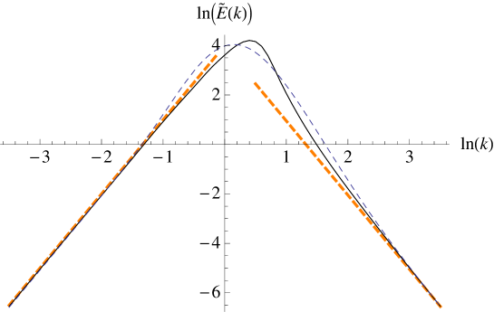
Figure 2: Double logarithmic plot for the rescaled energy $\tilde{E}(k):=k\tilde{\Delta}(k)$ as a function of $k$. The solid black line is our solution of equation (65); the thick dashed lines show the asymptotic slopes $\pm 3$. The thin grey-blue dashed line is $\tilde{E}_{\rm guess}(k):=k\tilde{\Delta}_{\rm guess}(k)$, see equation (85).

To find numerically a fixed-point solution $\tilde{\Delta}^{*}(u)$ of equation (65) is highly non-trivial. Since equation (65) is an integral-equation, none of the standard techniques, such as Taylor-expansion, or solution as an eigenvalue problem are available. From a decent physical fixed point, we expect that it is attractive w.r.t. all (sensible and small) perturbations. Thus, if we propose a guess $\tilde{\Delta}_{\mathrm{guess}}(u)$, which satisfies the above mentioned asymptotic behaviors and constraints, and is close to the true solution, it should converge against the fixed point. This is what we succeeded in doing, starting from $\Delta_{\mathrm{cor}}(k)=0$:

$$\tilde{\Delta}(k)=\tilde{\Delta}_{\mathrm{guess}}(k)+\tilde{\Delta}_{\mathrm{cor}}(k),$$ (84)

$$\tilde{\Delta}_{\mathrm{guess}}(k)=16\pi\left(\frac{k^{2}}{\left(k^{2}+1\right)^{3}}+\frac{54.7237k^{6}}{\left(k^{2}+1\right)^{6}}+\frac{2.65177k^{4}}{\left(k^{2}+1\right)^{5}}\right)\ .$$ (85)

The main problem then was that numerically the flow-equation (65) is rather unstable. The technique we finally succeeded in getting to work was: Starting with $\tilde{\Delta}_{\rm corr}(k)=0$, we recursively inject $\tilde{\Delta}_{\rm corr}(k)$ into the flow equation (65), and use the latter to evolve $\tilde{\Delta}(k)$ during a small time-step, giving us an improved approximation for $\tilde{\Delta}(k)$, calculated for approximately 100 $k$-points. The latter is then projected onto an optimal spline with only 20 supporting points, or more precisely a non-linear transformation thereof. This procedure is numerically much more stable than using a best polynomial fit, a Fourier representation, or any of the other known sets of orthogonal functions we tried. The projection effectively smoothes the function, while still capturing the necessary details. The complete technical details can be found in I, most importantly a check of the convergence of the function, see figure 9, as well as its tabulated values. Here we illustrate the result in the form of the classical double-logarithmic plot for the energy as a function of $k$, see figure 2. The small-$k$ asymptotics is $E(k)\sim k^{3}$, and the large-$k$ asymptotics is $E(k)\sim k^{-3}$. We remark that the solution remains below the asymptotic small-$k$ behavior, but then converges from above towards the asymptotic large-$k$ behavior.

6.2.6 Physical interpretation of the solution

We have found a fixed point $\tilde{\Delta}(k)$ for 2D decaying turbulence. Having in mind equation (72), the velocity-velocity correlation is $\Delta(k)=t^{2}\tilde{\Delta}(tk)$ where $\tilde{\Delta}$ is time independent. Thus

$$t\partial_{t}\Delta(k)=2\Delta(k)+k\Delta^{\prime}(k).$$ (86)

This implies similar relations for the time evolution of energy $E(k)=k\Delta(k)$ and enstrophy $\Omega(k)=k^{3}\Delta(k)$

$$t\partial_{t}E(k)=2k\Delta(k)+k^{2}\Delta^{\prime}(k)\ ,\qquad t\partial_{t}\Omega(k)=2k^{3}\Delta(k)+k^{4}\Delta^{\prime}(k)\ .$$ (87)

We define scaled momentum-dependent energy and enstrophy decay rates, written in terms of the scaled momentum $\tilde{k}=kt^{\zeta/2}=kt$ and correlator as:

$$\tilde{\dot{E}}(\tilde{k}):=\partial_{t}E(k)=2\tilde{k}\tilde{\Delta}(\tilde{k})+\tilde{k}^{2}\Delta^{\prime}(\tilde{k})=-\partial_{\tilde{k}}\tilde{j}_{E}(\tilde{k})$$ (88)

$$\tilde{\dot{\Omega}}(\tilde{k}):=t^{2}\partial_{t}\Omega(k)=2\tilde{k}^{3}\tilde{\Delta}(\tilde{k})+\tilde{k}^{4}\tilde{\Delta}^{\prime}(\tilde{k})=-\partial_{\tilde{k}}\tilde{j}_{\Omega}(\tilde{k})$$ (89)

where we have defined the scaled energy and enstrophy fluxes:

$$\tilde{j}_{E}(\tilde{k})=-\tilde{k}^{2}\tilde{\Delta}(\tilde{k})\quad,\quad\tilde{j}_{\Omega}(\tilde{k})=-\tilde{k}^{4}\tilde{\Delta}(\tilde{k})+2\int_{0}^{\tilde{k}}\rmd p\,p^{3}\,\tilde{\Delta}(p)$$ (90)

The scaled energy and enstrophy decay rates, and the scaled fluxes, all as functions of $\tilde{k}$ are plotted on figure 3. (For convenience we revert to the notation of the rest of the paper for the argument of $\tilde{\Delta}$, i.e. the $x$-axis is called $k$ but it is more properly $\tilde{k}$). We see that the energy flux $\tilde{j}_{E}(k)$ is negative, thus to small momentum scales, and moreover energy is conserved, since $\lim_{k\to\infty}\tilde{j}_{E}(k)=0$. Hence the total energy decay rate vanishes, $\bar{\epsilon}=-\partial_{t}{\cal E}=\frac{-1}{4\pi t}\int\rmd\tilde{k}\tilde{\dot{E}}(\tilde{k})=0$. The enstrophy flux is mostly positive, thus to large momentum scales, and enstrophy is not conserved. However, note that for $\Delta(k)\sim 1/k^{4}$, the integral in (90) grows as $\ln k$, thus the enstrophy conservation is only marginally violated. For $\Delta(k)\sim 1/[k^{4}(\ln k)^{c}]$, and $c>1$, the enstrophy would be conserved, since the flux at large $k$ would vanish. Thus a small modification of the asymptotic behavior, which might not be given correctly by our leading-order fixed point, would be enough to ensure enstrophy conservation.

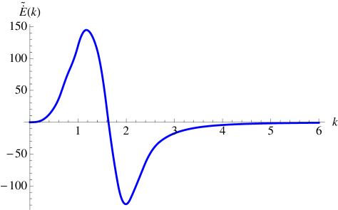
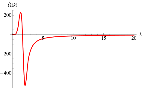
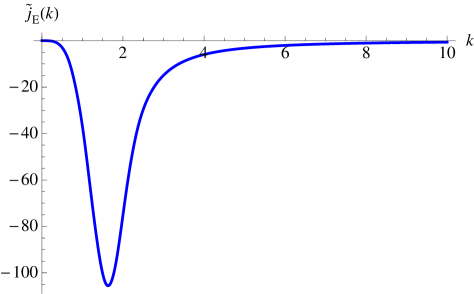
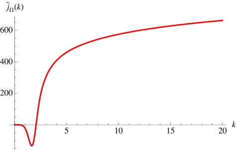
Figure 3: The scaled energy decay rate $\tilde{\dot{E}}$ and enstrophy $\tilde{\dot{\Omega}}$ (top) as well as their fluxes $\tilde{j}_{E}$ and $\tilde{j}_{\Omega}$ (bottom), defined in the text, as a function of the rescaled momentum (noted $k$ here).

To summarize, it seems that the FRG fixed point is compatible with the Batchelor-Kraichnan scenario [41, 93] with an enstrophy anomaly $-\partial_{t}\frac{1}{2}\langle{\omega_{{\bf u}t}^{2}}\rangle=\lim_{\nu\to 0}\nu\langle{(\nabla\omega)^{2}}\rangle=\bar{\epsilon}_{\omega}$. Since $\bar{\epsilon}_{\omega}$ has dimension $({\rm time})^{-3}$, the energy spectrum within the Batchelor-Kraichnan 2D enstrophy cascade is $E(k,t)\sim\bar{\epsilon}_{\omega}^{2/3}k^{-3}$, with, in decaying turbulence $\bar{\epsilon}_{\omega}\sim 1/t^{3}$. However, it is also known that this is not the end of the story, and that more detailed arguments and assumptions lead to additional logarithmic corrections, e.g. $E(k,t)\sim\bar{\epsilon}_{\omega}^{2/3}/(k^{3}(\ln k)^{c})$ with $c=1/3$ [93, 6]. It was also argued that in real space the vorticity correlations are  not $\langle(\omega_{{\bf u}}-\omega_{0})^{2}\rangle\sim\ln u$ at small scale, as would be the case if $E(k)\sim 1/k^{3}$. Instead they have fractional powers of $\ln u$, claimed to extend to all moments of the vorticity field, as $\langle(\omega_{{\bf u}}-\omega_{0})^{n}\rangle\sim(\ln u)^{n/3}$ [94], as a consequence of the infinite number of conservation laws; each conservation law is violated and leads to a flux of the corresponding (almost conserved) quantity. (Equivalently one can write that $\langle v\cdot\nabla\omega^{n}\omega^{n}\rangle$ is a constant [94]). Most of these issues were discussed for forced turbulence, but remain relevant for the decaying case. Note that in forced 2D turbulence there is an additional regime with an inverse energy cascade $E(k)\sim k^{-5/3}$ (see e.g. [6]). The energy flows to large scales, until the largest scale is reached, where coherent structures form. (These lowest $k$ modes may be called a condensate). At small scales however, the behavior should not be qualitatively different from decaying turbulence. For numerical and experimental tests of the enstrophy cascade see [95, 96, 97]. As discussed in [98, 99], friction is a marginal perturbation, hence should change the logarithms of the distance in the vorticity correlations into power laws. Finally, for a more mathematical discussion of the enstrophy anomaly see [100, 101]. In particular, the anomaly was proven to vanish in the forced 2D Euler equation with friction [102].

A challenging question is whether some of this physics can be captured in higher-loop extensions of the present approach.

6.3 Periodic 2D-turbulence

Let us consider the NS equation in a square box of size $L=2\pi$ with periodic boundary conditions. We study the FRG equation (26) for $N=2$, using integer Fourier modes $(k_{x},k_{y})\in\mathbb{Z}^{2}$, which are summed over. It is easy to analyze numerically the FRG equation projected onto a grid $[-Q,Q]^{2}$, setting $\Delta(k)=0$ outside. Equation (26) can be written schematically as $\partial_{\tau}R(k)=(R*R)(k)$ with $\tau=t^{2}/2$ and $R(k)=\Delta(k)/k^{2}$. Rescaling is not crucial here, since periodic turbulence corresponds to $\zeta=0$. One finds, for any $Q$, that the flow asymptotically behaves as

$$R(k)=r_{1}\delta_{k=(\pm 1,0),(0,\pm 1)}+\tilde{r}_{k}e^{-\lambda\tau}$$ (91)

and that the energy becomes entirely concentrated in the lowest modes $k^{2}=1$. The Fourier coefficient $r_{1}$ of these modes tends to a constant at large times, while all other modes decay. There is a transient regime where the other modes first increase before decaying, following (91). The $\tilde{r}_{k}$ are obtained by diagonalizing $\partial_{\tau}\tilde{r}_{k}=2(R_{1}*\tilde{r})(k)=-\lambda\tilde{r}_{k}$, where $R_{1}=r_{1}\delta_{k=(\pm 1,0),(0,\pm 1)}$ is a real non-symmetric matrix. We truncated numerically on a grid $k\in[-Q,Q]^{2}$ and found, apart from one trivial eigenvalue $\lambda=0,$ corresponding to $\tilde{R}=R_{1}$, that all eigenvalues are negative. Only the leading one corresponds to a vector with all positive entries for $k^{2}>1$, which is requested from (91). A plot of $\lambda$ versus $1/Q^{2}$ is approximately linear and the numerical solution suggests $\lambda=-0.6r_{1}$. The leading eigenvector is very well fitted by $\tilde{r}_{k}/\tilde{r}_{1}=1.57k^{-a}$ with $a=5.8\pm 1$, which we checked up to $Q=16$. Since $a>4$, this is consistent with the absence of an energy anomaly. It is interesting that this value of $a$ seems to be indeed near the Batchelor value of $a=6,$ which corresponds to $\Delta(k)\sim k^{-4}$ and $E(k)\sim k^{-3}$ [41], consistent with our analysis in the last section.

In conclusion, we want to note that $R(k)$ written in real space tends to a fixed point which corresponds to the average over the set of exact, time-independent solutions of the Euler equation,

$$\psi_{{\bf u}t}=w_{1x}\cos(u_{x})+w_{2x}\sin(u_{x})+w_{1y}\cos(u_{y})+w_{2y}\sin(u_{y}),$$ (92)

$${\bf v}_{{\bf u}t}=\big{(}-w_{1y}\sin(u_{y})+w_{2y}\cos(u_{y}),w_{1x}\sin(u_{x})-w_{2x}\cos(u_{x})\big{)}.$$ (93)

This is easily checked by inserting into Euler’s equation. The four parameters $w_{ix,y}$ are independent Gaussian random variables with zero mean and variance $r_{1}/2$. The FRG suggests that the way it tends to this fixed point is non-trivial (with a non-analytic correlator). It would be of great interest to study that question in detail.

7 Analysis of the FRG equation in three dimensions ($N=3$), and in large dimensions ($N\to\infty$)

Obtaining a numerical solution for the fixed point of the FRG equation for $N>2$ is difficult. In three dimension $N=3$ we have studied the FRG equation (26) for a periodic flow, in Fourier space, very much as we did in the previous Section for $N=2$. We have found that on a grid in Fourier space $[-Q,Q]^{3}$ equation (29) does flow to a fixed point with $\zeta=0$. This fixed point, to our numerical accuracy, was compatible with a cusp behavior at large $k$, i.e. $\zeta_{2}=1$. Since the result is not too surprising, and consistent with the analysis of Section 5, we will not reproduce the details here. Instead we now turn to the large dimension limit (large $N$ limit) analysis of the FRG equation.

Large dimensions are often a means of controlling an expansion. The aim would be to sum contributions from all loops at $N\to\infty$, thus avoiding any artifact from a closure scheme, as has been done for random manifolds, i.e., Burgers, [54, 103, 104, 105]. While this remains a project for future research, we have analyzed the one-loop equations for $N\to\infty$. In terms of the function $r(y)$ introduced in equation (31), the RG equations at large $N$ are derived in J and reads

$$N\left(2+N\right)t\partial_{t}{r}^{\prime\prime}({y})+4\,{y}\left[\left(2+N\right)t\partial_{t}{r}^{\prime\prime\prime}({y})+{y}t\partial_{t}{r}^{\prime\prime\prime\prime}({y})\right]=2r^{\prime\prime}({y})+\zeta_{0}yr^{\prime\prime\prime}({y})+{\ 2}r^{\prime\prime}({y})^{2}+{\ 2}r^{\prime\prime\prime}({y})\big{[}r^{\prime}({y})-r^{\prime}(0)\big{]}$$

$$+\frac{1}{N}\Big{[}4r^{\prime\prime}({y})+y(8+6\zeta_{0}+\zeta_{-1})r^{\prime\prime\prime}({y})+4\zeta_{0}y^{2}r^{\prime\prime\prime\prime}({y})+{\ 2}r^{\prime\prime}({y})^{2}+{\ 10}r^{\prime\prime\prime}({y})\big{[}r^{\prime}({y})-r^{\prime}(0)\big{]}$$

$$~{}~{}~{}~{}~{}~{}~{}+12yr^{\prime\prime\prime\prime}({y})\big{[}r^{\prime}({y})-r^{\prime}(0)\big{]}+28yr^{\prime\prime}({y})r^{\prime\prime\prime}({y})-4\int_{0}^{\infty}\rmd t\,r^{\prime\prime\prime}(y+t)r^{\prime\prime}(t)\Big{]}+O(1/N^{2}),$$ (94)

where $\zeta=\zeta_{0}+\zeta_{-1}/N+...$ We now look for a fixed point. To leading order we have

$$0=2r^{\prime\prime}(y)+\zeta_{0}yr^{\prime\prime\prime}(y)+{\ 2\big{[}}r^{\prime\prime}(y)\big{]}^{2}+{\ 2}r^{\prime\prime\prime}(y)\big{[}r^{\prime}(y)-r^{\prime}(0)\big{]},$$ (95)

which coincides, up to a numerical prefactor, with the large-$N$ limit of the 1-loop Burgers equation, see e.g. equation (7.7) of Ref. [104]. This confirms that at least to one loop the infinite-$N$ limit of the decaying Navier Stokes equation reproduces that of the Burgers equation. Equation (95) has an exponentially decaying solution only for $\zeta_{0}=0$; an analytic solution for the inverse function can be written as

$$z:=-r^{\prime}(y),$$ (96)

$$y=z-z_{0}-z_{0}\ln(z/z_{0}).$$ (97)

The asymptotic behavior is $z=z_{0}e^{-1-y/z_{0}}$ for large $y$. However, we cannot neglect the terms of order $1/N$ for $y/N\gg 1$, and the above solution is valid only for $y\ll N$, the primary region. On the other hand, for $y\gg z_{0}$, one can neglect the nonlinear terms in equation (95) due to the exponential decay of $r(y)$. Both solutions are expected to match in the inner region $z_{0}\ll y\ll N$, which becomes quite wide for $N\to\infty$ [77, 89]. Presumably in the inner region both solutions have a simple exponential behavior, to order $1/N$. The linearized equation to order $1/N$ reads

$$0=2r^{\prime\prime}(y)-{\ 2}r^{\prime\prime\prime}(y)r^{\prime}(0)+\frac{1}{N}\Big{[}4r^{\prime\prime}(y)+8yr^{\prime\prime\prime}(y)+\zeta_{-1}yr^{\prime\prime\prime}(y)-{\ 10}r^{\prime\prime\prime}(y)r^{\prime}(0)$$

$$\mbox{}\hskip 56.9055pt-{\ 12}yr^{\prime\prime\prime\prime}(y)r^{\prime}(0)-{\ 4}\int_{0}^{\infty}\rmd t\,r^{\prime\prime\prime}(y+t)r^{\prime\prime}(t)\Big{]}.$$ (98)

We assume that this equation has a solution which behaves as $e^{-y/z_{0}}$ for $y\gg z_{0}$. We are free to fix $z_{0}={\ 1}$ for the sake of simplicity. Substituting $r(y)=Ce^{-y}$ into the linearized equation, and collecting all terms proportional to $e^{-y}$ and $ye^{-y}$, we obtain

$$e^{-y}\ \ \ \ ~{}\,:\ \ \ \ 0=2+{\ 2}r^{\prime}(0)+\frac{1}{N}\Big{[}4+{\ 10}r^{\prime}(0)+2\int_{0}^{\infty}\rmd t\,e^{-t}r^{\prime\prime}(t)\Big{]},$$

$$ye^{-y}\ \ \ \ :\ \ \ \ 0=\frac{1}{N}\Big{[}-8-\zeta_{-1}-{\ 12}r^{\prime}(0)\Big{]}.$$ (99)

The first line gives $r^{\prime}(0)=-{\ 1}+O(1/N)$ and the second $\zeta_{-1}=4$, so that

$$\zeta=\frac{4}{N}+O\left(\frac{1}{N^{2}}\right).$$ (100)

Close to $z_{0}$ the solution of equation (97) has the form $z-z_{0}=\sqrt{2z_{0}y}\sim u$. This implies that the cusp persists, i.e. $\zeta_{2}=1$.

8 Decaying surface quasi-geostrophic turbulence

An interesting and still much studied generalization of 2D NS is the Surface Quasi Geostrophic (SQG) equation. It is defined in dimension $N=2$, and depends on a continuously varying parameter $a$. In real space it reads

$$\partial_{t}T_{{\bf u}t}+\mathbf{v}_{{\bf u}t}\cdot\nabla T_{{\bf u}t}=\nu\nabla^{2}T_{{\bf u}t}\ ,\quad\mathbf{v}_{{\bf u}t}=\hat{z}\times\nabla\psi_{{\bf u}t}\ ,\quad(-\nabla^{2})^{a/2}\psi_{{\bf u}t}=T_{{\bf u}t}.$$ (101)

It describes the convection of a quantity $T_{{\bf u}t}$ by the velocity field ${\bf v}_{{\bf u}t}$, which in turn is related to the velocity. For $a=2$ one recognizes that the quantity $T_{{\bf u}t}$ is precisely the vorticity $\omega_{{\bf u}t}$, and one recovers the usual 2D NS equation. For $a=1$ the field $T_{{\bf u}t}$ represents the temperature in the “true” SQG turbulence, which is used to model the 2D atmospheric flow on the surface of the Earth. Finally, for $a=-2$ the model was obtained by Charney and Oboukhov for waves in rotating fluids, and by Hasegawa and Mima for drift waves in a magnetized plasma in the limit of a vanishing Rossby radius. It is thus called the Charney-Hasegawa-Mima equation [106]. The naive scaling dimension of the field $T_{{\bf u}t}$ is $\delta_{u}T\sim u^{H}$ with $H=(2-2a)/3$. Recently, it has been conjectured that isolines of $T_{{\bf u}t}$ in the inverse-cascade regime of the forced Charney-Hasegawa-Mima equation were SLE lines with $\kappa=\frac{4}{3}(1+2a)$, with some numerical evidence [42, 107].

The SQG equation for arbitrary $a$ shares some properties with the 2D NS equation, in the sense that in the inviscid limit both the enstrophy $D=\frac{1}{2}\langle T^{2}\rangle$ (and all powers of $T$) and the energy $E=\frac{1}{2}\langle T\psi\rangle$ are conserved for flows smooth enough. To show the latter one goes to Fourier space, where the relation between $\psi_{{\bf u}t}$ and ${\bf v}_{{\bf u}t}$ is $\psi_{{\bf q}t}=q^{-a}T_{{\bf q}t}$. This yields

$$\partial_{t}E=\sum_{\bf q}T_{-{\bf q}t}q^{-a}\partial_{t}T_{{\bf q}t}=\sum_{{\bf k},{\bf q}}\frac{\epsilon_{\alpha\beta}{\bf k}_{\alpha}{\bf q}_{\beta}}{q^{a}k^{a}}T_{{\bf k}t}T_{{\bf q}-{\bf k}t}T_{-{\bf q}t}=0\ ,$$ (102)

due to the symmetry ${\bf q}\leftrightarrow-{\bf k}$.

Here we consider the decaying inviscid SQG equation. We display the FRG equation to one loop, leaving its analysis for the future. One defines the 2-point correlation in Fourier space,

$$\Delta_{T}({\bf k})=\langle{T_{-{\bf k}t}T_{{\bf k}t}}\rangle\ .$$ (103)

The FRG equation for $\Delta_{T}({\bf k})$ is derived in D, and reads

$$\partial_{t}\Delta_{T}({\bf k}) = t\sum_{\bf q}\Delta_{T}({\bf q})\Delta_{T}({\bf q}+{\bf k})[{\bf q}\times{\bf k}]^{2}\left\{q^{-2a}-2q^{-a}|{\bf q}+{\bf k}|^{-a}+|{\bf q}+{\bf k}|^{-2a}\right\}$$ (104)

$$-2t\sum_{\bf q}\Delta_{T}({\bf q})\Delta_{T}({\bf k})[{\bf q}\times{\bf k}]^{2}\left\{q^{-2a}-q^{-a}k^{-a}-q^{-a}|{\bf q}+{\bf k}|^{-a}+k^{-a}|{\bf q}+{\bf k}|^{-a}\right\}.$$

Note that the correlator associated to the velocity is $\Delta({\bf k})=k^{2-2a}\Delta_{T}({\bf k})$. Again, it is convenient to introduce the rescaled correlators via

$$\Delta_{T}({\bf k})=t^{-2+\frac{\zeta}{2}(6-2a)}\tilde{\Delta}_{T}({\bf k}t^{\zeta/2}),$$ (105)

$$\Delta({\bf k})=t^{-2+2\zeta}\tilde{\Delta}({\bf k}t^{\zeta/2}).$$ (106)

For the rescaled correlator, the FRG equation can be written as

$$\!\!\!\!\!t\partial_{t}\tilde{\Delta}_{T}({\bf k})=[2-(3-a)\zeta]\tilde{\Delta}_{T}({\bf k})-\frac{\zeta}{2}{\bf k}\partial_{{\bf k}}\tilde{\Delta}_{T}({\bf k})$$

$$~{}~{}~{}~{}~{}~{}~{}~{}~{}~{}~{}~{}~{}+\sum_{{\bf q},{\bf p}={\bf k}-{\bf q}}[{\bf q}\times{\bf k}]^{2}(q^{-a}-p^{-a})\tilde{\Delta}_{T}({\bf q})\Big{[}(q^{-a}-p^{-a})\tilde{\Delta}_{T}({\bf p})-2(q^{-a}-k^{-a})\tilde{\Delta}_{T}({\bf k})\Big{]}.$$ (107)

One can use ${\bf q}\times{\bf p}={\bf q}\times{\bf k}$. The equation for the rescaled velocity correlator reads

$$t\partial_{t}\tilde{\Delta}({\bf k})=(2-2\zeta)\tilde{\Delta}({\bf k})-\frac{\zeta}{2}{\bf k}\partial_{{\bf k}}\tilde{\Delta}({\bf k})$$

$$~{}~{}~{}~{}~{}~{}~{}~{}~{}~{}~{}~{}~{}+\sum_{{\bf q},{\bf p}={\bf k}-{\bf q}}\frac{[{\bf q}\times{\bf k}]^{2}}{q^{2}}\tilde{\Delta}({\bf q})\bigg{[}\frac{(p^{a}-q^{a})^{2}}{k^{2a-2}p^{2}}\tilde{\Delta}({\bf p})-2\frac{(p^{a}-q^{a})(k^{a}-q^{a})}{k^{a}p^{a}}\tilde{\Delta}({\bf k})\bigg{]}\ .$$ (108)

In this form it is easy to check that for $a=2$ one recovers the FRG equation for the NS equation in $N=2$.

The FRG equation (8) written in real space for general value of $a$ is a nonlocal integro-differential equation. It is interesting that there are some values of $a$ for which the FRG equation becomes quasi-local, i.e. involving only derivatives of finite order at the point ${\bf u}$ and at the origin ${\bf u}=0$. For instance that happens in the case of the Charney-Hasegawa-Mima turbulence corresponding to $a=-2$.

In F.3 we have studied, as we did for Burgers and NS, the possible values for the exponent $\zeta_{2}$, defined from $\tilde{\Delta}({\bf k})\sim k^{-(2+\zeta_{2})}$ at large $k$, and isotropic turbulence. More work is necessary to study the fixed points of the FRG equation as a function of the parameter $a$.

9 Conclusions and Perspectives

In this article, we have applied functional-renormalization-group methods to decaying turbulence. In contrast to standard perturbative RG, the functional RG approach takes into account a coupling function i.e. an infinity of couplings rather than one or few. It naturally leads to a non-analytic 2-point function. While the method is in principle exact, as any RG treatment, in practice the flow has to be projected onto a lower-dimensional subspace, here the equal-time 2-point velocity correlation function. With this projection in mind, the FRG equations are organized in an expansion in powers of the 2-point velocity correlation function itself, equivalent to a loop expansion. As we have discussed, they correspond to a small-time renormalized perturbation theory. Here, we studied the 1-loop equations. For Burgers, they reproduce the FRG equations derived in the context of random manifolds, and correctly describe the singular structure of the flow, made out of shocks. While this had been worked out in details before for $N=1$, here we extended it to any dimension $N$.

Let us stress that the method works at least qualitatively for Burgers; that it correctly accounts for shocks, and that the distribution of velocities is not close to a Gaussian. The reason is that the extension to a manifold provides a model which can be controlled perturbatively (in $d=4-\epsilon$), while at the same time exhibiting shock singularities, non-conservation of energy (called failure of dimensional reduction in the context of disordered systems) and energy cascades. This is because shock sizes and the magnitude of the energy decay rate are $O(\epsilon)$ in that expansion. That in itself is remarkable in the turbulence context, and motivated us to consider Navier-Stokes with this method.

For Navier Stokes, the fixed point depends on the dimension. For $N\to\infty$, the FRG equations converge (at leading 1-loop order) to those of the decaying Burgers equation. Thus the 2-point velocity correlation function should grow linearly with distance, i.e. have a cusp. This cusp is also the only possible solution for the 3-dimensional FRG equation, at 1-loop order, in contradiction to experimental evidence. It is possible, that at second (2-loop) or higher order, new non-trivial fixed points emerge. If this is not the case, one would have to understand why the method seemingly does not admit the correct singularities. Since for large $N$ we find that the FRG equation reduces to the one of Burgers, hence has shock singularities, one possible way to understand that may be via a large-dimension expansion combined with a loop expansion.

Finally, in two dimensions the FRG equations allow for a fixed point which is consistent with Batchelor’s scaling. While the equations are similar to the quasi-normal Markovian approximation, we give here an explicit solution. Again it seems a good starting point to include higher-loop corrections, one challenge being to confirm, or infirm, the conjectured logarithmic corrections. We have also written the flow equations corresponding to SQG turbulence, which await a more detailed analysis.

We hope that this work helps to bring a new perspective in a long-debated subject.

Acknowlegments: We thank D. Bernard, B. Birnir, and I. Procaccia for useful discussions. We are especially indebted to B. Shraiman and G. Falkovich for many enlightening remarks. This work was supported by ANR under two successive programs, 05-BLAN-0099-01 and 09-BLAN-0097-01/2, and in part through NSF grants PHY05-51164 and PHY11-25915 during several stays at KITP. We also thank the KITPC for its hospitality.

Appendix A 1-loop FRG equation in real space

The two equations from (13) needed to one loop in the inviscid limit are

$$\qquad\quad\ \ \partial_{t}\Delta_{\alpha_{1}\alpha_{2}}({\bf u}) = {\rm Sym}\Big{[}P_{\alpha_{1};\beta\gamma}(\partial_{{\bf u}})C^{(3)}_{\beta\gamma\alpha_{2}}(0,0,{\bf u})\Big{]}=-{\rm Sym}\Big{[}P_{\alpha_{1};\beta\gamma}(\partial_{{\bf u}})C^{(3)}_{\beta\gamma\alpha_{2}}({\bf u},{\bf u},0)\Big{]}$$ (109)

$$= 2\,{\rm Sym}\Big{[}P^{\rm T}_{\alpha_{1}\beta}(\partial_{{\bf u}})\partial_{{\bf u}}^{\gamma}C^{(3)}_{\beta\gamma\alpha_{2}}(0,0,{\bf u})\Big{]}\qquad\quad~{}~{}~{}({\rm Euler})$$ (110)

$$= {\rm Sym}\Big{[}\partial_{{\bf u}}^{\alpha_{1}}C^{(3)}_{\beta\beta\alpha_{2}}(0,0,{\bf u})\Big{]}\qquad\qquad\qquad\quad({\rm Burgers})$$ (111)

$$\partial_{t}C^{(3)}_{\alpha_{1}\alpha_{2}\alpha_{3}}({\bf u}_{1},{\bf u}_{2},{\bf u}_{3}) = -\frac{3}{2}{\rm Sym}\Big{[}P_{\alpha_{1}\beta\gamma}(\partial_{{\bf u}_{1}})C^{(4)}_{\beta\gamma\alpha_{2}\alpha_{3}}({\bf u}_{1},{\bf u}_{1},{\bf u}_{2},{\bf u}_{3})\Big{]}$$ (112)

with ${\bf u}={\bf u}_{12}$ and where $P_{\alpha;\beta\gamma}(\partial)=P^{\rm T}_{\alpha\beta}(\partial)\partial_{\gamma}+P^{\rm T}_{\alpha\gamma}(\partial)\partial_{\beta}$ (Euler), $P_{\alpha;\beta\gamma}(\partial)=\delta_{\beta\gamma}\partial_{\alpha}$ (Burgers). In the first three lines ${\rm Sym}[...]$ means symmetrization over $\alpha_{1},\alpha_{2}$ and we have used that $\Delta_{\alpha_{1}\alpha_{2}}({\bf u})$ is even in ${\bf u}$ (no average helicity). In the last line, and everywhere below ${\rm Sym}[...]$ means symmetrization over ${\bf u}_{1}^{\alpha_{1}},{\bf u}_{2}^{\alpha_{2}},{\bf u}_{3}^{\alpha_{3}}$, i.e simultaneous exchange of the points in space and the indices.

To lowest order we replace (denoting ${\bf u}_{ij}:={\bf u}_{i}-{\bf u}_{j}$)

$$C^{(4)}_{\beta\gamma\alpha_{2}\alpha_{3}}({\bf u}_{1},{\bf u}_{1},{\bf u}_{2},{\bf u}_{3})=\Delta_{\beta\gamma}(0)\Delta_{\alpha_{2}\alpha_{3}}({\bf u}_{23})+\Delta_{\beta\alpha_{2}}({\bf u}_{12})\Delta_{\gamma\alpha_{3}}({\bf u}_{13})+\Delta_{\beta\alpha_{3}}({\bf u}_{13})\Delta_{\gamma\alpha_{2}}({\bf u}_{12})\ .$$ (113)

Hence integrating equation (112) one gets

$$\!\!\!\!\!\!\!\!\!\!\!\!\!\!\!\!\!\!\!\!\!\!\!\!\!\!\!\!\!\!\!\!\!\!\!\!\!\!\!\!\!\!\!C^{(3)}_{\alpha_{1}\alpha_{2}\alpha_{3}}({\bf u}_{1},{\bf u}_{2},{\bf u}_{3})=-\frac{3}{2}t\,{\rm Sym}\Big{[}P_{\alpha_{1}\beta\gamma}(\partial_{{\bf u}_{1}})\Big{(}\Delta_{\beta\alpha_{2}}({\bf u}_{12})\Delta_{\gamma\alpha_{3}}({\bf u}_{13})\Big{)}+P_{\alpha_{1}\beta\gamma}(\partial_{{\bf u}_{1}})\Big{(}\Delta_{\beta\alpha_{3}}({\bf u}_{13})\Delta_{\gamma\alpha_{2}}({\bf u}_{12})\Big{)}\Big{]}$$

$$=-3t\,{\rm Sym}\Big{[}P^{\rm T}_{\alpha_{1}\gamma}(\partial_{{\bf u}_{1}})\Big{(}\Delta_{\beta\alpha_{3}}({\bf u}_{13})\partial_{{\bf u}_{1}}^{\beta}\Delta_{\gamma\alpha_{2}}({\bf u}_{12})+\Delta_{\beta\alpha_{2}}({\bf u}_{12})\partial_{{\bf u}_{1}}^{\beta}\Delta_{\gamma\alpha_{3}}({\bf u}_{13})\Big{)}\Big{]}\quad~{}~{}~{}({\rm Euler})$$ (114)

$$=-3t\,{\rm Sym}\Big{[}\partial_{{\bf u}_{1}}^{\alpha_{1}}\big{(}\Delta_{\beta\alpha_{2}}({\bf u}_{12})\Delta_{\beta\alpha_{3}}({\bf u}_{13})\big{)}\Big{]}\quad~{}~{}~{}~{}~{}~{}~{}~{}~{}~{}~{}~{}~{}~{}~{}~{}~{}~{}~{}~{}~{}~{}~{}~{}~{}~{}~{}~{}~{}~{}~{}~{}~{}~{}~{}~{}~{}~{}~{}~{}~{}~{}~{}~{}~{}~{}~{}~{}~{}~{}~{}~{}({\rm Burgers})$$ (115)

where for Euler we used the transversality of $\Delta_{\alpha\beta}$. Expanding, one finds for Burgers

$$-t^{-1}C^{(3)}_{\alpha_{1}\alpha_{2}\alpha_{3}}({\bf u}_{1},{\bf u}_{2},{\bf u}_{3})=\partial_{{\bf u}_{1}}^{\alpha_{1}}\Big{(}\Delta_{\beta\alpha_{2}}({\bf u}_{12})\Delta_{\beta\alpha_{3}}({\bf u}_{13})\Big{)}+\partial_{{\bf u}_{2}}^{\alpha_{2}}\Big{(}\Delta_{\beta\alpha_{1}}({\bf u}_{21})\Delta_{\beta\alpha_{3}}({\bf u}_{23})\Big{)}+\partial_{{\bf u}_{3}}^{\alpha_{3}}\Big{(}\Delta_{\beta\alpha_{2}}({\bf u}_{32})\Delta_{\beta\alpha_{1}}({\bf u}_{31})\Big{)}.$$

This expression is symmetric and does not need to be symmetrized. Taking the limit of ${\bf u}_{2}\to{\bf u}_{1}$ one finds

$$-t^{-1}C^{(3)}_{\alpha_{1}\alpha_{2}\alpha_{3}}({\bf u}_{1},{\bf u}_{1},{\bf u}_{3})=\partial_{{\bf u}_{3}}^{\alpha_{3}}\Big{(}\Delta_{\beta\alpha_{2}}({\bf u}_{31})\Delta_{\beta\alpha_{1}}({\bf u}_{31})\Big{)}+\Delta_{\beta\alpha_{2}}(0)\partial_{{\bf u}_{1}}^{\alpha_{1}}\Delta_{\beta\alpha_{3}}({\bf u}_{13})+\Delta_{\beta\alpha_{1}}(0)\partial_{{\bf u}_{2}}^{\alpha_{2}}\Delta_{\beta\alpha_{3}}({\bf u}_{23})\ .$$ (117)

We have used that

$$\lim_{{\bf u}_{2}\to{\bf u}_{1}}\big{(}\partial_{{\bf u}_{1}}^{\alpha_{1}}\Delta_{\beta\alpha_{2}}({\bf u}_{12})\big{)}\Delta_{\beta\alpha_{3}}({\bf u}_{13})+\big{(}\partial_{{\bf u}_{2}}^{\alpha_{2}}\big{(}\Delta_{\beta\alpha_{1}}({\bf u}_{21})\big{)}\Delta_{\beta\alpha_{3}}({\bf u}_{23})=0\ ,$$ (118)

which comes from $R^{\prime\prime\prime}_{\alpha_{1}\beta\alpha_{2}}({\bf u})$ being odd. One then gets

$$\partial_{t}\Delta_{\alpha_{1}\alpha_{2}}({\bf u})=-t\partial_{{\bf u}}^{\alpha_{1}}\partial_{{\bf u}}^{\alpha_{2}}\Delta_{\beta\beta^{\prime}}({\bf u})^{2}+2t\Delta_{\beta\beta^{\prime}}(0)\Delta_{\beta\alpha_{2};\beta^{\prime}\alpha_{1}}({\bf u})\ ,$$ (119)

where we have used that $\Delta_{\beta\alpha_{2};\beta^{\prime}}({\bf u})$ is odd and that $\Delta_{\beta\alpha_{2};\beta^{\prime}\alpha_{1}}({\bf u})=-R^{\prime\prime\prime\prime}_{\beta\beta^{\prime}\alpha_{1}\alpha_{2}}({\bf u})$ is symmetric in $\alpha_{1},\alpha_{2}$. This gives the equation in the text.

For Euler one finds by expanding

$$-t^{-1}C^{(3)}_{\alpha_{1}\alpha_{2}\alpha_{3}}({\bf u}_{1},{\bf u}_{2},{\bf u}_{3}) = P^{\rm T}_{\alpha_{1}\gamma}(\partial_{{\bf u}_{1}})\big{(}\Delta_{\beta\alpha_{3}}({\bf u}_{13})\partial_{{\bf u}_{1}}^{\beta}\Delta_{\gamma\alpha_{2}}({\bf u}_{12})+\Delta_{\beta\alpha_{2}}({\bf u}_{12})\partial_{{\bf u}_{1}}^{\beta}\Delta_{\gamma\alpha_{3}}({\bf u}_{13})\big{)}$$ (120)

$$+P^{\rm T}_{\alpha_{2}\gamma}(\partial_{{\bf u}_{2}})\big{(}\Delta_{\beta\alpha_{3}}({\bf u}_{23})\partial_{{\bf u}_{2}}^{\beta}\Delta_{\gamma\alpha_{1}}({\bf u}_{21})+\Delta_{\beta\alpha_{1}}({\bf u}_{21})\partial_{{\bf u}_{2}}^{\beta}\Delta_{\gamma\alpha_{3}}({\bf u}_{23})\big{)}$$

$$+P^{\rm T}_{\alpha_{3}\gamma}(\partial_{{\bf u}_{3}})\big{(}\Delta_{\beta\alpha_{1}}({\bf u}_{31})\partial_{{\bf u}_{3}}^{\beta}\Delta_{\gamma\alpha_{2}}({\bf u}_{32})+\Delta_{\beta\alpha_{2}}({\bf u}_{32})\partial_{{\bf u}_{3}}^{\beta}\Delta_{\gamma\alpha_{1}}({\bf u}_{31})\big{)}\ .$$

This expression is symmetric and does not need to be symmetrized. We now take the limit ${\bf u}_{2}\to{\bf u}_{1}$:

$$-t^{-1}C^{(3)}_{\beta\gamma\alpha_{2}}({\bf u}_{1},{\bf u}_{1},{\bf u}_{3}) = P^{\rm T}_{\alpha_{2}\gamma^{\prime}}(\partial_{{\bf u}_{3}})\big{(}\Delta_{\beta^{\prime}\beta}({\bf u}_{31})\partial_{{\bf u}_{3}}^{\beta^{\prime}}\Delta_{\gamma^{\prime}\gamma}({\bf u}_{31})+\Delta_{\beta^{\prime}\gamma}({\bf u}_{31})\partial_{{\bf u}_{3}}^{\beta^{\prime}}\Delta_{\gamma^{\prime}\beta}({\bf u}_{31})\big{)}$$ (121)

$$+\lim_{{\bf u}_{2}\to{\bf u}_{1}}\bigg{(}P^{\rm T}_{\beta\gamma^{\prime}}(\partial_{{\bf u}_{1}})\Big{(}\Delta_{\beta^{\prime}\alpha_{2}}({\bf u}_{13})\partial_{{\bf u}_{1}}^{\beta^{\prime}}\Delta_{\gamma^{\prime}\gamma}({\bf u}_{12})+\Delta_{\beta^{\prime}\gamma}({\bf u}_{12})\partial_{{\bf u}_{1}}^{\beta^{\prime}}\Delta_{\gamma^{\prime}\alpha_{2}}({\bf u}_{13})\Big{)}$$

$$\qquad~{}~{}~{}~{}~{}~{}+P^{\rm T}_{\gamma\gamma^{\prime}}(\partial_{{\bf u}_{2}})\Big{(}\Delta_{\beta^{\prime}\alpha_{2}}({\bf u}_{23})\partial_{{\bf u}_{2}}^{\beta^{\prime}}\Delta_{\gamma^{\prime}\beta}({\bf u}_{21})+\Delta_{\beta^{\prime}\beta}({\bf u}_{21})\partial_{{\bf u}_{2}}^{\beta^{\prime}}\Delta_{\gamma^{\prime}\alpha_{2}}({\bf u}_{13})\Big{)}\bigg{)}\ .$$

The term $\lim_{{\bf u}_{2}\to{\bf u}_{1}}\big{(}...\big{)}$ involves a non-trivial coinciding-point limit. One may naively equate it with

$$P^{\rm T}_{\beta\gamma^{\prime}}(\partial_{{\bf u}_{1}})\Delta_{\beta^{\prime}\gamma}(0)\partial_{{\bf u}_{1}}^{\beta^{\prime}}\Delta_{\gamma^{\prime}\alpha_{2}}({\bf u}_{13})+P^{\rm T}_{\gamma\gamma^{\prime}}(\partial_{{\bf u}_{1}})\Delta_{\beta^{\prime}\beta}(0)\partial_{{\bf u}_{1}}^{\beta^{\prime}}\Delta_{\gamma^{\prime}\alpha_{2}}({\bf u}_{13})\ ,$$ (122)

but this is actually incorrect. It would lead to a term $+2t\Delta_{\beta^{\prime}\gamma}(0)\partial_{{\bf u}}^{\beta^{\prime}}\partial_{{\bf u}}^{\gamma}\Delta_{\alpha_{1}\alpha_{2}}({\bf u})$ in the beta function. The correct beta function must retain the non-trivial limit, for which we obtain, with ${\bf u}_{31}={\bf u}$:

$$\partial_{t}\Delta_{\alpha_{1}\alpha_{2}}({\bf u})=2[P^{\rm T}_{\alpha_{1}\beta}(\partial_{{\bf u}})\partial_{{\bf u}}^{\gamma}C^{(3)}_{\beta\gamma\alpha_{2}}(0,0,{\bf u})]$$

$$=-2tP^{\rm T}_{\alpha_{1}\beta}(\partial_{{\bf u}})P^{\rm T}_{\alpha_{2}\gamma^{\prime}}(\partial_{{\bf u}})\big{(}\partial_{{\bf u}}^{\gamma}\Delta_{\beta^{\prime}\beta}({\bf u})\partial_{{\bf u}}^{\beta^{\prime}}\Delta_{\gamma^{\prime}\gamma}({\bf u})+\Delta_{\beta^{\prime}\gamma}({\bf u})\partial_{{\bf u}}^{\gamma}\partial_{{\bf u}}^{\beta^{\prime}}\Delta_{\beta\gamma^{\prime}}({\bf u})\big{)}$$

$$~{}~{}~{}~{}+2t\,{\rm Sym}\Big{[}P^{\rm T}_{\alpha_{1}\beta}(\partial_{{\bf u}})\partial_{{\bf u}}^{\gamma}P^{\rm T}_{\alpha_{2}\gamma^{\prime}}(\partial_{{\bf u}_{3}})\lim_{{\bf u}_{2}\to{\bf u}_{1}}\Big{(}P^{\rm T}_{\beta\gamma^{\prime}}(\partial_{{\bf u}_{1}})\big{(}\Delta_{\beta^{\prime}\alpha_{2}}({\bf u}_{13})\partial_{{\bf u}_{1}}^{\beta^{\prime}}\Delta_{\gamma^{\prime}\gamma}({\bf u}_{12})+\Delta_{\beta^{\prime}\gamma}({\bf u}_{12})\partial_{{\bf u}_{1}}^{\beta^{\prime}}\Delta_{\gamma^{\prime}\alpha_{2}}({\bf u}_{13})\big{)}$$

$$\qquad~{}~{}~{}~{}~{}~{}~{}~{}~{}~{}~{}+P^{\rm T}_{\gamma\gamma^{\prime}}(\partial_{{\bf u}_{2}})(\Delta_{\beta^{\prime}\alpha_{2}}({\bf u}_{23})\partial_{{\bf u}_{2}}^{\beta^{\prime}}\Delta_{\gamma^{\prime}\beta}({\bf u}_{21})+\Delta_{\beta^{\prime}\beta}({\bf u}_{21})\partial_{{\bf u}_{2}}^{\beta^{\prime}}\Delta_{\gamma^{\prime}\alpha_{2}}({\bf u}_{13})\Big{)}\Big{]}\ .$$ (123)

We have used that $\partial_{{\bf u}}^{\beta^{\prime}}\Delta_{\gamma^{\prime}\alpha_{2}}({\bf u})$ is odd, and several times transversality i.e.  $\Delta_{\alpha\beta}({\bf u})=P^{\rm T}_{\alpha\beta}(\partial_{{\bf u}})R(u)$ (this does not assume any symmetry) hence $P^{\rm T}_{\alpha_{1}\gamma^{\prime}}(\partial_{{\bf u}})\Delta_{\gamma^{\prime}\alpha_{2}}(u)=\Delta_{\alpha_{1}\alpha_{2}}(u)$.

Appendix B 1-loop FRG equation in Fourier space

To one loop one must first solve

$$\partial_{t}C^{(3)}_{\alpha_{1}\alpha_{2}\alpha_{3}}({\bf k}_{1},{\bf k}_{2},{\bf k}_{3})=-\frac{3}{2}{\rm Sym}\Big{[}P_{\alpha_{1};\beta\gamma}({\bf k}_{1})\sum_{{\bf p}+{\bf q}={\bf k}_{1}}C^{(4)}_{\beta\gamma\alpha_{2}\alpha_{3}}({\bf p},{\bf q},{\bf k}_{2},{\bf k}_{3})\Big{]}\ ,$$ (124)

where again, here and below ${\rm Sym}[...]$ means symmetrization w.r.t ${\bf k}_{1}^{\alpha_{1}},{\bf k}_{2}^{\alpha_{2}},{\bf k}_{2}^{\alpha_{2}}$ (simultaneous permutations of points and indices). Here $P_{\alpha;\beta\gamma}({\bf k})=i{\bf k}^{\beta}P^{\rm T}_{\alpha\gamma}({\bf k})+i{\bf k}^{\gamma}P^{\rm T}_{\alpha\beta}({\bf k})$ for NS and $P_{\alpha;\beta\gamma}({\bf k})=i{\bf k}^{\alpha}\delta_{\beta\gamma}$ for Burgers, and one uses the Gaussian approximation

$$C^{(4)}_{\beta\gamma\alpha_{2}\alpha_{3}}({\bf p},{\bf q},{\bf k}_{2},{\bf k}_{3}) = \delta_{{\bf p}+{\bf q}}\delta_{{\bf k}_{2}+{\bf k}_{3}}\Delta_{\beta\gamma}({\bf p})\Delta_{\alpha_{2}\alpha_{3}}({\bf k}_{2})$$ (125)

$$+\delta_{{\bf p}+{\bf k}_{2}}\delta_{{\bf q}+{\bf k}_{3}}\Delta_{\beta\alpha_{2}}({\bf p})\Delta_{\gamma\alpha_{3}}({\bf q})+\delta_{{\bf p}+{\bf k}_{3}}\delta_{{\bf q}+{\bf k}_{2}}\Delta_{\beta\alpha_{3}}({\bf p})\Delta_{\gamma\alpha_{2}}({\bf q})\ .$$

We assume that $\Delta_{\alpha\beta}(-{\bf k})=\Delta_{\alpha\beta}({\bf k})$. The first term vanishes when multiplied by $P_{\alpha_{1};\beta\gamma}({\bf k}_{1})$. One finds, using symmetries

$$C^{(3)}_{\alpha_{1}\alpha_{2}\alpha_{3}}({\bf k}_{1},{\bf k}_{2},{\bf k}_{3}) = \delta_{{\bf k}_{1}+{\bf k}_{2}+{\bf k}_{3}}\hat{C}^{(3)}_{\alpha_{1}\alpha_{2}\alpha_{3}}({\bf k}_{1},{\bf k}_{2},{\bf k}_{3})$$ (126)

$$\hat{C}^{(3)}_{\alpha_{1}\alpha_{2}\alpha_{3}}({\bf k}_{1},{\bf k}_{2},{\bf k}_{3}) = -t\Big{(}P_{\alpha_{1}\beta\gamma}({\bf k}_{1})\Delta_{\beta\alpha_{2}}({\bf k}_{2})\Delta_{\gamma\alpha_{3}}({\bf k}_{3})$$ (127)

$$\ \ \ \ \ \ +P_{\alpha_{2}\beta\gamma}({\bf k}_{2})\Delta_{\beta\alpha_{1}}({\bf k}_{1})\Delta_{\gamma\alpha_{3}}({\bf k}_{3})+P_{\alpha_{3}\beta\gamma}({\bf k}_{3})\Delta_{\beta\alpha_{1}}({\bf k}_{1})\Delta_{\gamma\alpha_{2}}({\bf k}_{2})\Big{)}\ .$$

This expression is already symmetric and does not need symmetrization anymore.

The 1-loop equation is obtained by inserting this result into

$$\partial_{t}\Delta_{\alpha_{1}\alpha_{2}}({\bf k}) = -{\rm Sym}\Big{[}P_{\alpha_{1}\beta^{\prime}\gamma^{\prime}}({\bf k})\sum_{{\bf p}+{\bf q}={\bf k}}\hat{C}^{(3)}_{\beta^{\prime}\gamma^{\prime}\alpha_{2}}({\bf p},{\bf q},-{\bf k})\Big{]}$$

$$= t\,{\rm Sym}\Big{[}P_{\alpha_{1}\beta^{\prime}\gamma^{\prime}}({\bf k})\Delta_{\gamma\alpha_{2}}({\bf k})\sum_{{\bf p}+{\bf q}={\bf k}}P_{\beta^{\prime}\beta\gamma}({\bf p})\Delta_{\beta\gamma^{\prime}}({\bf q})+P_{\alpha_{1}\beta^{\prime}\gamma^{\prime}}({\bf k})\Delta_{\gamma\alpha_{2}}({\bf k})\sum_{{\bf p}+{\bf q}={\bf k}}P_{\gamma^{\prime}\beta\gamma}({\bf q})\Delta_{\beta\beta^{\prime}}({\bf p})$$

$$~{}~{}~{}~{}~{}~{}~{}~{}~{}~{}-P_{\alpha_{1}\beta^{\prime}\gamma^{\prime}}({\bf k})P_{\alpha_{2}\beta\gamma}({\bf k})\sum_{{\bf p}+{\bf q}={\bf k}}\Delta_{\beta\beta^{\prime}}({\bf p})\Delta_{\gamma\gamma^{\prime}}({\bf q})\Big{]}\ ,$$

where here ${\rm Sym}[...]$ means symmetrization w.r.t. $\alpha_{1},\alpha_{2}$. Symmetrization finally yields the general 1-loop equation

$$\partial_{t}\Delta_{\alpha_{1}\alpha_{2}}({\bf k}) = t\bigg{(}\Big{(}P_{\alpha_{1}\beta^{\prime}\gamma^{\prime}}({\bf k})\Delta_{\gamma\alpha_{2}}({\bf k})+P_{\alpha_{2}\beta^{\prime}\gamma^{\prime}}({\bf k})\Delta_{\gamma\alpha_{1}}({\bf k})\Big{)}\sum_{{\bf p}+{\bf q}={\bf k}}P_{\beta^{\prime}\beta\gamma}({\bf p})\Delta_{\beta\gamma^{\prime}}({\bf q})$$ (129)

$$~{}~{}-P_{\alpha_{1}\beta^{\prime}\gamma^{\prime}}({\bf k})P_{\alpha_{2}\beta\gamma}({\bf k})\sum_{{\bf p}+{\bf q}={\bf k}}\Delta_{\beta\beta^{\prime}}({\bf p})\Delta_{\gamma\gamma^{\prime}}({\bf q})\bigg{)}\ ,$$

from which the 1-loop FRG equation for NS and Burgers can be retrieved.

For NS one has ${\bf k}_{\alpha_{i}}\Delta_{\alpha_{1},\alpha_{2}}({\bf k})=0$ for $i=1,2$. One checks on (129) that if $\Delta$ is transverse at a given time $t$, it remains so, i.e.  the r.h.s. is automatically transverse. For $N=2$ this implies that $\Delta_{\alpha\beta}({\bf k})=P^{\rm T}_{\alpha\beta}({\bf k})\Delta({\bf k})$, but this is not true for $N>2$. The general form is $\Delta_{\alpha\beta}({\bf k})=\sum_{i,j=1}^{N-1}e_{\alpha}^{i}({\bf k})e_{\beta}^{j}({\bf k})\Delta_{ij}({\bf k})$ where the $e^{i}({\bf k})$ span a basis orthogonal to ${\bf k}$ and $\Delta_{ij}({\bf k})$ is a symmetric matrix.

For simplicity we consider here the subspace $\Delta_{\alpha\beta}({\bf k})=P^{\rm T}_{\alpha\beta}({\bf k})\Delta({\bf k})$. One finds, using Mathematica

$$\sum_{{\bf p}+{\bf q}={\bf k}}P_{\alpha_{1}\beta^{\prime}\gamma^{\prime}}({\bf k})P_{\alpha_{2}\beta\gamma}({\bf k})\Delta_{\beta\beta^{\prime}}({\bf p})\Delta_{\gamma\gamma^{\prime}}({\bf q})=\frac{-2}{N-1}P^{\rm T}_{\alpha_{1}\alpha_{2}}({\bf k})\sum_{q}\frac{[k^{2}q^{2}-({\bf k}\cdot{\bf q})^{2}]}{k^{2}q^{2}({\bf k}-{\bf q})^{2}}$$

$$\times\Big{[}\frac{1}{2}\Big{(}({\bf k}-{\bf q})^{2}-q^{2}\Big{)}^{2}+\frac{1}{2}(N-2)k^{2}\Big{(}q^{2}+({\bf k}-{\bf q})^{2}\Big{)}\Big{]}\Delta({\bf q})\Delta({\bf k}-{\bf q})\ .$$ (130)

At this stage this was obtained by: (i) symmetrizing w.r.t. $q\to k-q,$ and (ii) assuming that the result was proportional to $P^{\rm T}_{\alpha_{1}\alpha_{2}}({\bf k}),$ and then contracting with $P^{\rm T}_{\alpha_{1}\alpha_{2}}({\bf k})$ (or $\delta_{\alpha_{1},\alpha_{2}}$). For $N=2$ there is no loss of generality, and the sum over momenta can be discrete, while for $N>2$ this holds only for isotropic turbulence $\Delta({\bf k})=\Delta(k)$ and in the limit of an infinite box where the sums become integrals.

Next one finds by the same method

$$\Big{(}P_{\alpha_{1}\beta^{\prime}\gamma^{\prime}}({\bf k})\Delta_{\gamma\alpha_{2}}({\bf k})+P_{\alpha_{2}\beta^{\prime}\gamma^{\prime}}({\bf k})\Delta_{\gamma\alpha_{1}}({\bf k})\Big{)}\sum_{{\bf p}+{\bf q}={\bf k}}P_{\beta^{\prime}\beta\gamma}({\bf p})\Delta_{\beta\gamma^{\prime}}({\bf q})$$ (131)

$$=\frac{-2}{N-1}P^{\rm T}_{\alpha_{1}\alpha_{2}}({\bf k})\sum_{q}\frac{k^{2}q^{2}-({\bf k}\cdot{\bf q})^{2}}{k^{2}q^{2}({\bf k}-{\bf q})^{2}}\Big{[}(k^{2}-q^{2})\Big{(}({\bf k}-{\bf q})^{2}-q^{2}\Big{)}+(N-2)k^{2}({\bf k}-{\bf q})^{2}\Big{]}\Delta({\bf q})\Delta({\bf k})\ .$$

This yields the 1-loop FRG equation

$$\partial_{t}\Delta({\bf k})=\frac{2t}{N-1}\sum_{q}\frac{k^{2}q^{2}-({\bf k}\cdot{\bf q})^{2}}{k^{2}q^{2}({\bf k}-{\bf q})^{2}}\Bigg{\{}\Big{[}\frac{1}{2}\Big{(}({\bf k}-{\bf q})^{2}-q^{2}\Big{)}^{2}+\frac{1}{2}(N-2)k^{2}\Big{(}q^{2}+({\bf k}-{\bf q})^{2}\Big{)}\Big{]}\Delta({\bf q})\Delta({\bf k}-{\bf q})$$

$$\hbox to0.0pt{\hss${}-{}$}\Big{[}(k^{2}-q^{2})\Big{(}({\bf k}-{\bf q})^{2}-q^{2}\Big{)}+(N-2)k^{2}({\bf k}-{\bf q})^{2}\Big{]}\Delta({\bf q})\Delta({\bf k})\Bigg{\}}\ .$$ (132)

We note Kraichnan’s conventions,

$$4k^{2}a_{{\bf k},{\bf p},{\bf q}}=P_{\alpha_{1}\beta^{\prime}\gamma^{\prime}}({\bf k})P_{\alpha_{1}\beta\gamma}({\bf k})P^{\rm T}_{\beta\beta^{\prime}}({\bf p})P^{\rm T}_{\gamma\gamma^{\prime}}({\bf q})\ ,$$ (133)

$$2k^{2}b_{{\bf k},{\bf p},{\bf q}}=P_{cjm}({\bf k})P_{jbc}({\bf p})P^{\rm T}_{mb}({\bf q})\ .$$ (134)

This corrects a misprint in equation (VII-2-7) of [6]. The various symbols satisfy

$$2\tilde{a}_{{\bf k},{\bf k}-{\bf q},{\bf q}}=-4k^{2}a_{{\bf k},{\bf k}-{\bf q},{\bf q}}=\frac{[k^{2}q^{2}-({\bf k}\cdot{\bf q})^{2}]}{k^{2}q^{2}({\bf k}-{\bf q})^{2}}\Big{[}\Big{(}({\bf k}-{\bf q})^{2}-q^{2}\Big{)}^{2}+(N-2)k^{2}\Big{(}q^{2}+({\bf k}-{\bf q})^{2}\Big{)}\Big{]}$$ (135)

$$\tilde{b}_{{\bf k},{\bf k}-{\bf q},{\bf q}}=-2k^{2}b_{{\bf k},{\bf k}-{\bf q},{\bf q}}=\frac{[k^{2}q^{2}-({\bf k}\cdot{\bf q})^{2}]}{k^{2}q^{2}({\bf k}-{\bf q})^{2}}\Big{[}(k^{2}-q^{2})\Big{(}({\bf k}-{\bf q})^{2}-q^{2}\Big{)}+(N-2)k^{2}({\bf k}-{\bf q})^{2}\Big{]}$$ (136)

$$\tilde{a}_{{\bf k},{\bf k}-{\bf q},{\bf q}}=\frac{1}{2}\left[\tilde{b}_{{\bf k},{\bf k}-{\bf q},{\bf q}}+\tilde{b}_{{\bf k},{\bf q},{\bf k}-{\bf q}}\right]\ .$$ (137)

The FRG equation can thus be written in various forms,

$$\partial_{t}\Delta({\bf k}) = \frac{2t}{N-1}\sum_{q}\tilde{a}_{{\bf k},{\bf k}-{\bf q},{\bf q}}\Delta({\bf q})\Delta({\bf k}-{\bf q})-\tilde{b}_{{\bf k},{\bf k}-{\bf q},{\bf q}}\Delta({\bf q})\Delta({\bf k})\ ,$$ (138)

as well as the form given in the text.

Note that $\tilde{b}_{{\bf k},{\bf k}-{\bf q},{\bf q}}$ is not invariant under ${\bf q}\to{\bf k}-{\bf q}$; $\tilde{a}_{{\bf k},{\bf k},0}=\tilde{a}_{{\bf k},0,{\bf k}}=\frac{1}{2}\tilde{b}_{{\bf k},{\bf k},0}$ while $\tilde{b}_{{\bf k},0,{\bf k}}=0$. These properties imply that the coefficient $B$ in the expansions in the text is zero. Further $k^{2}q^{2}-({\bf k}\cdot{\bf q})^{2}=k^{2}p^{2}-({\bf k}\cdot{\bf p})^{2}=p^{2}q^{2}-({\bf p}\cdot{\bf q})^{2}$ if ${\bf k}={\bf p}+{\bf q}$, hence this term is already symmetric under ${\bf q}\to{\bf k}-{\bf q}$.

Appendix C FRG equation for $N=3$ periodic flows

A convenient parameterization of a general $N=3$ divergence-less velocity correlation matrix, i.e.  such that ${\bf k}_{\alpha}\Delta_{\alpha\beta}({\bf k})=0$, (with mirror symmetry) is

$$\Delta_{\alpha\beta}({\bf k}) = \sum_{i=x,y,z}\epsilon_{\alpha i\gamma}\hat{\bf k}_{\gamma}\epsilon_{\beta i\delta}\hat{\bf k}_{\delta}\Delta_{i}({\bf k})$$ (139)

$$=\delta_{\alpha\beta}\left(\sum_{i}\Delta_{i}({\bf k})(1-\hat{\bf k}_{i}^{2})-\Delta_{\alpha}({\bf k})\right)-\hat{\bf k}_{\alpha}\hat{\bf k}_{\beta}\left(\sum_{i}\Delta_{i}({\bf k})-\Delta_{\alpha}({\bf k})-\Delta_{\beta}({\bf k})\right)\ .$$

In coordinates this is

$$\Delta_{xx}({\bf k})=\hat{\bf k}_{y}^{2}\Delta_{z}({\bf k})+\hat{\bf k}_{z}^{2}\Delta_{y}({\bf k})\quad,\quad\Delta_{xy}({\bf k})=\Delta_{yx}({\bf k})=-\hat{\bf k}_{x}\hat{\bf k}_{y}\Delta_{z}({\bf k})\ ,$$ (140)

and similar for circular permutations. The semi-isotropic case $\Delta_{\alpha\beta}({\bf k})=P^{\rm T}_{\alpha\beta}({\bf k})\Delta({\bf k})$ corresponds to $\Delta_{i}({\bf k})=\Delta({\bf k}),$ and is fully isotropic when $\Delta_{i}({\bf k})=\Delta(|{\bf k}|)$. For a periodic flow with a cubic lattice symmetry we expect that

$$\Delta_{x}({\bf k})=\Delta({\bf k}_{y},{\bf k}_{z};{\bf k}_{x})\quad,\quad\Delta_{y}({\bf k})=\Delta({\bf k}_{x},{\bf k}_{z};{\bf k}_{y})\quad,\quad\Delta_{z}({\bf k})=\Delta({\bf k}_{x},{\bf k}_{y};{\bf k}_{z})$$ (141)

where $\Delta({\bf k}_{1},{\bf k}_{2};{\bf k}_{3})$ is a symmetric function of its first two arguments.

We have derived FRG equations for the $\Delta_{i}$. They are of the form $\partial\Delta_{z}=\sum_{i,j=x,y,z}\sum_{q}\Delta_{i}({\bf q})\Delta_{j}({\bf k}-{\bf q})f_{ij}({\bf k},{\bf q})$ where the $f_{ij}({\bf k},{\bf q})$ are quite complicated functions of $k_{x},k_{y},k_{z},q_{x},q_{y},q_{z}$; we have not tried to solve them.

Appendix D Generating functional approach and diagrammatics

In this appendix we explain how the FRG equations can be derived for the decaying Burgers, NS and SQG equations within the Martin-Siggia-Rose formalism, using a small-time expansion. We start with the Burgers equation, with an initial condition ${\bf v}_{{\bf u}0}={\bf w}_{\bf u}$ at $t=0^{+}$. This is equivalent to

$$\partial_{t}{\bf v}_{{\bf u}t}+\frac{1}{2}\nabla_{{\bf u}}{\bf v}_{{\bf u}t}^{2}=\nu\nabla^{2}_{{\bf u}}{\bf v}_{{\bf u}t}+\delta(t){\bf w}_{\bf u}\ ,$$ (142)

with ${\bf v}_{{\bf u}t}=0$ for $t<0$, i.e. a forcing which acts only at time zero. We then introduce the generating functional $e^{-S[{\bf v}_{{\bf u}t},\tilde{{\bf v}}_{{\bf u}t}]}$ for the velocity correlators, in the usual way, which leads to the dynamic action

$$S = \int_{{\bf u},t\geq 0}\Big{[}\tilde{\bf v}_{{\bf u}t}\partial_{t}{\bf v}_{{\bf u}t}-\nu\tilde{\bf v}_{{\bf u}t}\nabla_{{\bf u}}^{2}{\bf v}_{{\bf u}t}-\ \frac{1}{2}(\nabla_{{\bf u}}\cdot\tilde{\bf v}_{{\bf u}t})({\bf v}_{{\bf u}t})^{2}\Big{]}-\int_{\bf u}\tilde{\bf v}_{{\bf u}0}{\bf w}_{\bf u}\ .$$ (143)

$\tilde{\bf v}_{{\bf u}t}$ is the response field, and the path integral should be evaluated with ${\bf v}_{{\bf u}t=0^{-}}=0$ at the boundary. Since normalization of the path integral is one, the generating function for averages over the initial conditions can be computed from the dynamical path integral with action:

$$S^{\prime} = \int_{{\bf u},t\geq 0}\Big{[}\tilde{\bf v}_{{\bf u}t}\partial_{t}{\bf v}_{{\bf u}t}-\nu\tilde{\bf v}_{{\bf u}t}\nabla_{{\bf u}}^{2}{\bf v}_{{\bf u}t}-\ \frac{1}{2}(\nabla_{{\bf u}}\cdot\tilde{\bf v}_{{\bf u}t})({\bf v}_{{\bf u}t})^{2}\Big{]}-\frac{1}{2}\int_{{\bf u},{\bf u}^{\prime}}\tilde{{\bf v}}_{{\bf u}0}^{\alpha}\Delta^{0}_{\alpha\beta}({\bf u}-{\bf u}^{\prime})\tilde{{\bf v}}_{{\bf u}^{\prime}0}^{\beta},$$ (144)

where $\langle{{\bf w}_{\bf u}^{\alpha}{\bf w}_{{\bf u}^{\prime}}^{\beta}}\rangle=\Delta^{0}_{\alpha\beta}({\bf u}-{\bf u}^{\prime})$. We use the following graphical representation. The vertex corresponding to the cubic nonlinearity is depicted by

$$-(\partial_{{\bf u}}^{\beta}\tilde{\bf v}_{{\bf u}t}^{\beta})({\bf v}_{{\bf u}t}^{\alpha}{\bf v}_{{\bf u}t}^{\alpha})=\parbox{58.20059pt}{\hskip 3.44444pt\includegraphics[scale={0.35}]{./Burgersaind}\hskip 3.44444pt}\ .$$ (145)

The response function in the limit $\nu\to 0$ reads

$$\Theta(t_{2}-t_{1})\delta_{\alpha\beta}=\parbox{162.26938pt}{\hskip 3.44444pt\includegraphics[scale={0.35}]{./response}\hskip 3.44444pt}\ .$$ (146)

The dashed line denotes the 2-point velocity correlator at $t=0$,

$$\Delta^{0}_{\alpha\beta}({\bf u}-{\bf u}^{\prime})=\parbox{162.26938pt}{\hskip 3.44444pt\includegraphics[scale={0.35}]{./initial}\hskip 3.44444pt}.$$ (147)

We now switch to the Fourier representation. The 2-point velocity correlator written in Fourier space $\Delta_{\alpha\beta}^{t}({\bf k})=\langle{{\bf v}_{{\bf k}t}^{\alpha}{\bf v}_{-{\bf k}t}^{\beta}}\rangle$ to 1-loop order is given by the diagrams

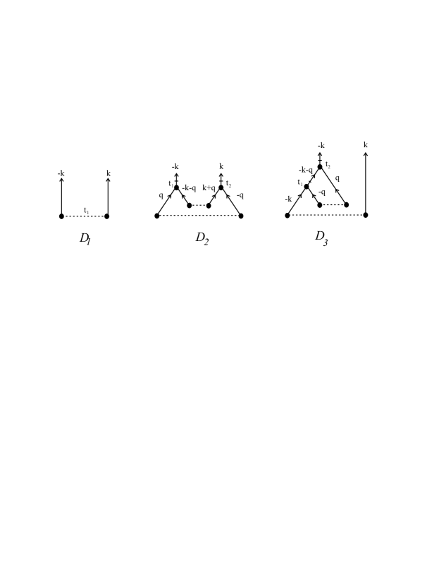
Figure 4: The diagrams given in Eqs. (148) to (150).

given on figure 4. The corresponding expressions with combinatorial factors are

$$D_{1}=\Delta^{0}_{\alpha\beta}({\bf k}),$$ (148)

$$D_{2}=\frac{t^{2}}{2}{\bf k}_{\alpha}{\bf k}_{\beta}\sum_{\bf q}\Delta^{0}_{\gamma\delta}({\bf q})\Delta^{0}_{\gamma\delta}({\bf k}+{\bf q}),$$ (149)

$$D_{3}=-t^{2}{\bf k}_{\alpha}{\bf k}_{\beta}\sum_{\bf q}\Delta^{0}_{\gamma\delta}({\bf q})\Delta^{0}_{\gamma\delta}({\bf k}).$$ (150)

In real space, the sum of the diagrams can be written as

$$\Delta_{\alpha\beta}^{t}({\bf u}) = \Delta_{\alpha\beta}^{0}({\bf u})-\frac{t^{2}}{2}\partial_{\alpha}\partial_{\beta}[\Delta_{\gamma\delta}^{0}({\bf u})-\Delta_{\gamma\delta}^{0}(0)]^{2}.$$ (151)

To compute the $\beta$-function we take the derivative with respect to $t$

$$\partial_{t}\Delta_{\alpha\beta}^{t}({\bf u}) = -t\partial_{\alpha}\partial_{\beta}[\Delta_{\gamma\delta}^{0}({\bf u})-\Delta_{\gamma\delta}^{0}(0)]^{2}\ ,$$ (152)

and substitute to one loop $\Delta_{\alpha\beta}^{0}=\Delta_{\alpha\beta}^{t}$. As a result we obtain the FRG equation (18).

We now generalize the method developed above to the Navier-Stokes equation. It is convenient to put all derivatives in the cubic vertex on the response field and write the dynamical action as

$$S=\int_{{\bf u},t\geq 0}\Big{[}\tilde{\bf v}_{{\bf u}t}\partial_{t}{\bf v}_{{\bf u}t}-\nu\tilde{\bf v}_{{\bf u}t}\nabla_{{\bf u}}^{2}{\bf v}_{{\bf u}t}-\lambda{\bf v}_{{\bf u}t}^{\beta}{\bf v}_{{\bf u}t}^{\gamma}(P^{\rm T}_{\alpha\beta}(\partial_{{\bf u}})\partial^{\gamma}_{{\bf u}}\tilde{\bf v}_{{\bf u}t}^{\alpha})\Big{]}-\frac{1}{2}\int_{{\bf u},{\bf u}^{\prime}}\tilde{{\bf v}}_{{\bf u}0}^{\alpha}\Delta^{0}_{\alpha\beta}(u-u^{\prime})\tilde{{\bf v}}_{{\bf u}^{\prime}0}^{\beta}\ ,\ \ \ \ \$$ (153)

where the last term imposes the initial condition similar to that in action (144). The nonlinear cubic vertex can then be written as

$${\bf v}_{{\bf u}t}^{\beta}{\bf v}_{{\bf u}t}^{\alpha}(P^{\rm T}_{\beta\beta^{\prime}}(\partial_{{\bf u}})\partial^{\alpha}_{{\bf u}}\tilde{\bf v}_{{\bf u}t}^{\beta^{\prime}})=\parbox{46.63739pt}{\hskip 3.44444pt\includegraphics[scale={0.35}]{./turbvertInd3}\hskip 3.44444pt}=-\parbox{46.63739pt}{\hskip 3.44444pt\includegraphics[scale={0.35}]{./turbvertInd2}\hskip 3.44444pt}\ .$$ (154)

The two-point function $\Delta_{\alpha\beta}^{t}({\bf k})=\langle{{\bf v}_{{\bf k}t}^{\alpha}{\bf v}_{-{\bf k}t}^{\beta}}\rangle$ to second order in $\Delta^{0}({\bf k})$ is given by the diagrams in figure 5. The tree-level diagram $S_{1}$ reads

$$S_{1}=\Delta^{0}_{\alpha\beta}({\bf k}).$$ (155)

There are six 1PI one-loop diagrams which can be split into two groups. The first group gives

$$S_{2}+S_{3} = t^{2}P^{\mathrm{T}}_{\alpha\gamma}(-{\bf k})P^{\mathrm{T}}_{\beta\sigma}({\bf k}){\bf k}_{\delta}{\bf k}_{\rho}\sum_{{\bf q}}\Big{[}\Delta^{0}_{\gamma\sigma}({\bf q})\Delta^{0}_{\delta\rho}({\bf q}+{\bf k})+\Delta^{0}_{\gamma\rho}({\bf q})\Delta^{0}_{\delta\sigma}({\bf q}+{\bf k})\Big{]}.$$ (156)

Expanding the projection operators we find

$$P^{\mathrm{T}}_{\alpha\beta}({\bf k})[S_{2}+S_{3}]=t^{2}\sum_{\bf q}\tilde{a}_{{\bf k},{\bf k}-{\bf q},{\bf q}}\Delta^{0}({\bf q})\Delta^{0}({\bf k}+{\bf q}),$$

where we used that $\Delta^{0}_{\alpha\beta}({\bf q})=P^{\mathrm{T}}_{\alpha\beta}({\bf q})\Delta^{0}({\bf q})$ and $\tilde{a}$ is given by equation (135). Analogously we obtain

$$S_{4}+S_{5}+S_{6}+S_{7}=-t^{2}I_{\alpha\tau}({\bf k})\Delta^{0}_{\tau\beta}({\bf k}),$$ (157)

where we have introduced

$$I_{\alpha\tau}(k) = \sum_{\bf q}\left[P^{\mathrm{T}}_{\alpha\gamma}({\bf k})P^{\mathrm{T}}_{\gamma\tau}({\bf k}+{\bf q})P^{\mathrm{T}}_{\mu\sigma}(q)\Delta({\bf q}){\bf k}_{\sigma}({\bf k}_{\mu}+{\bf q}_{\mu})\right.$$ (158)

$$\left.~{}~{}~{}~{}~{}+P^{\mathrm{T}}_{\alpha\gamma}({\bf k})P^{\mathrm{T}}_{\gamma\mu}({\bf k}+{\bf q})P^{\mathrm{T}}_{\mu\sigma}({\bf q})\Delta({\bf q}){\bf k}_{\sigma}({\bf k}_{\tau}+{\bf q}_{\tau})\right.$$

$$\left.~{}~{}~{}~{}~{}+P^{\mathrm{T}}_{\alpha\sigma}({\bf k})P^{\mathrm{T}}_{\gamma\tau}({\bf k}+{\bf q})P^{\mathrm{T}}_{\mu\sigma}({\bf q})\Delta({\bf q}){\bf k}_{\gamma}({\bf k}_{\mu}+{\bf q}_{\mu})\right.$$

$$\left.~{}~{}~{}~{}~{}+P^{\mathrm{T}}_{\alpha\sigma}({\bf k})P^{\mathrm{T}}_{\gamma\mu}({\bf k}+{\bf q})P^{\mathrm{T}}_{\mu\sigma}({\bf q})\Delta({\bf q}){\bf k}_{\gamma}({\bf k}_{\tau}+{\bf q}_{\tau})\right].$$

Expanding the projection operators one sees that

$$P^{\mathrm{T}}_{\alpha\beta}({\bf k})[S_{4}+S_{5}+S_{6}+S_{7}]=-t^{2}\sum_{\bf q}\tilde{b}_{{\bf k},{\bf k}-{\bf q},{\bf q}}\Delta^{0}({\bf q})\Delta^{0}({\bf k}),$$

where $\tilde{b}$ is defined in equation (136). Taking the derivative with respect to $t$ we obtain the FRG equation (26).

The FRG equation for the SQG equation can be obtained in the same way. The dynamic action corresponding to equation (101) with the initial condition imposed at $t=0$ is given by

$$S=\int_{{\bf u},t\geq 0}\Big{\{}\tilde{T}_{{\bf u}t}\partial_{t}T_{{\bf u}t}-\nu\tilde{T}_{{\bf u}t}\nabla^{2}T_{{\bf u}t}+\tilde{T}_{{\bf u}t}\hat{z}\cdot[\nabla\psi_{{\bf u}t}\times\nabla T_{{\bf u}t}]\Big{\}}-\frac{1}{2}\int_{{\bf u},{\bf u}^{\prime}}\tilde{T}_{{\bf u}0}\Delta^{0}_{T}({\bf u}-{\bf u}^{\prime})\tilde{T}_{{\bf u}^{\prime}0}.\ \ \ \$$ (159)

The SQG vertex can be written in Fourier space as

$$\int_{{\bf u},t}\tilde{T}_{{\bf u}t}\hat{z}\cdot[\nabla\psi_{{\bf u}t}\times\nabla T_{{\bf u}t}]=\int_{{\bf u},{\bf u}^{\prime},t}\tilde{T}_{{\bf u}t}\epsilon_{\alpha\beta}\partial_{{\bf u}}^{\alpha}K_{{\bf u}-{\bf u}^{\prime}}{T}_{{\bf u}^{\prime}t}\partial_{{\bf u}}^{\beta}{T}_{{{\bf u}}t}$$

$$=-\int_{{\bf u},{\bf u}^{\prime},t}K_{{\bf u}-{\bf u}^{\prime}}{T}_{{\bf u}^{\prime}t}\epsilon_{\alpha\beta}\partial_{{\bf u}}^{\alpha}[\tilde{T}_{{\bf u}t}\partial_{{\bf u}}^{\beta}{T}_{{\bf u}t}]=-\int_{t}\sum_{{\bf k},{\bf q}}\tilde{T}_{-{\bf k}-{\bf q}t}\epsilon_{\alpha\beta}{\bf q}_{\alpha}{\bf k}_{\beta}q^{-a}T_{{\bf q}t}T_{{\bf k}t},$$ (160)

where we have introduced the inverse Fourier transform

$$K_{{\bf u}}:=\mbox{FT}^{-1}_{{\bf u}\leftarrow{\bf q}}\frac{1}{q^{a}}\ .$$ (161)

The 2-point function $\Delta^{t}_{T}({\bf k})=\langle{T_{{\bf k}t}T_{-{\bf k}t}}\rangle$ to second order in $\Delta^{0}_{T}$ is given by the diagrams in figure 5. The corresponding expressions read

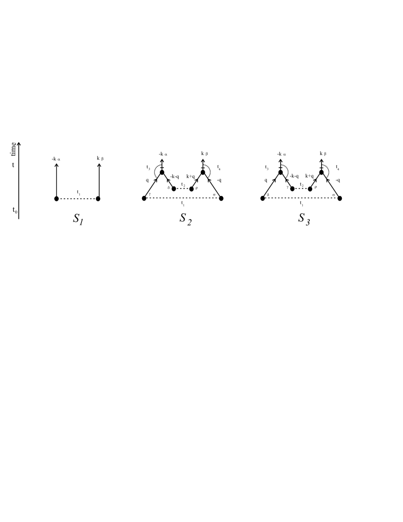
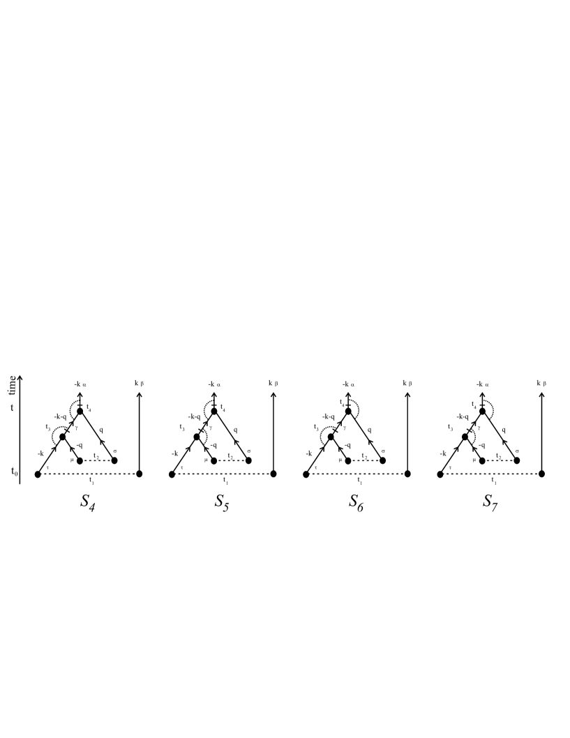
Figure 5: Diagrams contributing to the FRG for the NS and SQG equations.

$$~{}~{}~{}~{}~{}~{}~{}~{}~{}~{}~{}~{}~{}~{}~{}~{}~{}~{}~{}~{}S_{1} = \Delta_{T}^{0}({\bf k}),$$ (162)

$$~{}~{}~{}~{}~{}~{}~{}~{}~{}~{}~{}~{}~{}~{}S_{2}+S_{3} = \frac{1}{2}t^{2}\sum_{\bf q}\Delta^{0}_{T}({\bf q})\Delta^{0}_{T}({\bf q}+{\bf k})[{\bf q}\times{\bf k}]^{2}\left\{q^{-2a}-2q^{-a}|{\bf q}+{\bf k}|^{-a}+|{\bf q}+{\bf k}|^{-2a}\right\},$$ (163)

$$S_{4}+S_{5}+S_{6}+S_{7} = -t^{2}\sum_{\bf q}\Delta^{0}_{T}({\bf q})\Delta^{0}_{T}({\bf k})[{\bf q}\times{\bf k}]^{2}\left\{q^{-2a}-q^{-a}k^{-a}-q^{-a}|{\bf q}+{\bf k}|^{-a}+k^{-a}|{\bf q}+{\bf k}|^{-a}\right\}.$$ (164)

Taking the derivative with respect to $t$ and reexpressing the bare disorder$\Delta^{0}_{T}$ in terms of the renormalized one $\Delta_{T}$ we obtain the FRG equation (104).

Appendix E Distance geometry for FRG equation

E.1 Navier-Stokes

We derive the measure used in [6], e.g. equation (VII-2-9). Following [108], appendix A, the integral of a function $f(x_{1},\dots,x_{n})$ which depends only on $u_{ij}:=x_{i}\cdot x_{j}$ can be written as

$$\int_{\mathbb{R}^{N}}\prod_{i=1}^{n}\rmd^{N}x_{i}\,f(u_{ij})={S_{N}\over 2}\ldots{S_{N-n+1}\over 2}\int\prod_{i\leq j}\rmd u_{ij}(\det[u_{ij}])^{N-n-1\over 2}\ f([u_{ij}]),$$ (165)

where the domain of integration is such that the scalar-products can be realized in $N$-dimensional space, and $S_{N}=2\pi^{N/2}/\Gamma(N/2)$ is the area of the unit sphere. Here we need $n=2$ with ${\bf k}={\bf x}_{1}$, ${\bf p}={\bf x}_{2}$, ${\bf k}+{\bf p}+{\bf q}=0$, $k=|{\bf k}|$, $q=|{\bf q}|$, $p=|{\bf p}|$. One finds, for arbitrary $N$,

$$\int\rmd^{N}k\,\rmd^{N}p\,f(u_{ij}) = \int\rmd k^{2}\rmd p^{2}\rmd({\bf k}{\bf p})(k^{2}p^{2}-({\bf k}{\bf p})^{2})^{\frac{N-3}{2}}\frac{S_{N}S_{N-1}}{4}f(k^{2},p^{2},({\bf k}-{\bf p})^{2})$$ (166)

$$= S_{N}S_{N-1}\int_{\Delta}\rmd k\,\rmd p\,\rmd q\,kpq\,\left[\frac{4}{(p{+}q{-}k)(k{+}p{-}q)(k{+}q{-}p)(k{+}p{+}q)}\right]^{\frac{3-N}{2}}\,f(k^{2},p^{2},q^{2}),$$

where the triangle symbolizes the realization of the triangle inequality. We have used that ${\bf k}\cdot{\bf p}=\frac{1}{2}(p^{2}+k^{2}-q^{2})$ hence $\rmd k^{2}\rmd p^{2}\rmd({\bf k}{\bf p})=\frac{1}{2}\rmd k^{2}\rmd p^{2}\rmd q^{2}$, as well as,

$$k^{2}p^{2}-({\bf k}{\bf p})^{2}=\frac{1}{4}(k+p+q)(p+q-k)(k+p-q)(k-p+q).$$ (167)

The domain of integration is plotted in figure 6. A non-trivial check is to suppose that $f$ is independent of $p$, and to do the $p$ integration. With the domain in figure 6, the two cases $q<k$ and $q>k$ have to be distinguished. For $N=3$, both (!) give $\int p\,\rmd p=2kq$, which result in two independent 3-dimensional integrals (with correct normalization) for $q$ and $k$.

Since this is valid for any function of $k$, we may rewrite (26) for the isotropic case and any $N$, replacing $\sum_{q}\to\int_{q}=\int\frac{\rmd^{N}q}{(2\pi)^{N}}$, using $\delta\Delta(K)=\int\rmd^{N}{\bf k}\frac{\delta(k-K)}{S_{N}k^{N-1}}\delta\Delta(k)$, which yields

$$\!\!\!\!\!\!\!\!\!\!\!\!\!\!\!\!\!\!\!\!\!\!\!\!\!\!\!\!\!\!\!\!\!\!\!\!\partial_{t}\Delta(k)=\frac{2t}{N-1}\frac{S_{N-1}}{(2\pi)^{N}}\int_{0}^{\infty}\rmd q\int_{0}^{\infty}\rmd p\,\Theta_{\Delta}(k,p,q)\frac{B_{k,p,q}}{k^{N}pq}\left[\Delta(q)\Delta(p)-\Delta(q)\Delta(k)\right],$$ (169)

$$\!\!\!\!\!\!\!\!\!\!\!\!\!\!\!\!\!\!\!\!\!\!\!\!\!\!\!\!\!\!\!\!\!\!\!\!B_{kpq}=\left[\frac{1}{4}(k+p+q)(p+q-k)(k+p-q)(k-p+q)\right]^{\frac{N-1}{2}}\left[(k^{2}-q^{2})(p^{2}-q^{2})+(N-2)k^{2}p^{2}\right],$$

$$\!\!\!\!\!\!\!\!\!\!\!\!\!\!\!\!\!\!\!\!\!\!\!\!\!\!\!\!\!\!\!\!\!\!\!\!\Theta_{\Delta}(k,p,q)=\Theta(k+p>q)\Theta(k+q>p)\Theta(p+q>k).$$

The domain of integration is plotted in figure 6. The distance geometry can be parameterized by $p=\frac{k}{2}(s+t)$ and $q=\frac{k}{2}(s-t)$ with

$$\!\!\!\!\!\!\!\!\!\!\!\!\!\!\!\int_{0}^{\infty}\rmd p\int_{0}^{\infty}\rmd q~{}\Theta_{\Delta}(k,p,q)f(k,p,q)=\frac{k^{2}}{2}\int_{1}^{\infty}\rmd s\int_{-1}^{1}\rmd tf\big{(}k,\frac{k}{2}(s+t),\frac{k}{2}(s-t)\big{)}.$$ (170)

It is immediate from (169) that $\int_{0}^{\infty}\rmd k\,k^{N-1}\Delta(k)$ is conserved, using the symmetry under the exchange $p\leftrightarrow k$. This implies energy conservation for all $N$. For $N=2$ one checks that enstrophy is conserved, i.e.  $\int_{0}^{\infty}\rmd k\,k^{3}\Delta(k)$ can be brought to the form $\sim\int_{k,p,q}B_{kpq}(\frac{k}{pq}-\frac{p}{kq})\Delta(p)\Delta(q)$ which leads to a factor of $(k^{2}-p^{2})(k^{2}-q^{2})(p^{2}-q^{2})$ times a symmetric function of $p,q$; hence it vanishes.

Violation of energy conservation necessitates a divergence in the integrals for large momenta so that the operations involved in the symmetrization, e.g. change of order in integration, are no more valid. For $N=3$ one sees that at $\zeta_{2}=1$, for fixed $s$ and $t$ there is a logarithmic divergence $\int\rmd k/k$ at large $k$, none for $\zeta_{2}>1$, and a relevant one for $\zeta_{2}<1$. The momentum space-integrals are therefore no longer well-defined for $\zeta_{2}\leq 1$.

Figure 6: The domain of integration in equation (166).

E.2 Burgers

One finds a similar expression for Burgers:

$$\partial_{t}\Delta(k) = \frac{S_{N-1}t}{4(2\pi)^{N}}k^{2-N}\int_{0}^{\infty}\rmd q\int_{0}^{\infty}\rmd p\,\Theta_{\Delta}(k,p,q)\frac{1}{pq}\,\left[\frac{4}{(p{+}q{-}k)(k{+}p{-}q)(k{+}q{-}p)(k{+}p{+}q)}\right]^{\frac{3-N}{2}}\,$$ (171)

$$~{}~{}~{}~{}~{}~{}~{}~{}~{}~{}~{}~{}~{}~{}~{}~{}~{}~{}~{}~{}\times\bigg{[}\frac{k^{2}}{2}(p^{2}+q^{2}-k^{2})^{2}\Delta(p)\Delta(q)-p^{2}(k^{2}+q^{2}-p^{2})^{2}\Delta(q)\Delta(k)\bigg{]}.$$

Appendix F Short-distance expansion of $\Delta(u)$: Amplitudes $B$ and $C$ for Burgers, Navier Stokes and surface quasi-geostrophic turbulence

In this appendix, we calculate the necessary integrals for the short-distance expansion of $\Delta(u)$ for Burgers, F.1, Navier-Stokes, F.2 and quasi-geostrophic, F.3. For simplicity of notations, we use

$$b=N+\zeta_{2}\ .$$ (172)

F.1 Burgers

To get the coefficient $C$ in (58) we need to compute

$$J(k)=\frac{1}{2}k^{2}\int_{\bf q}\frac{[{\bf q}\cdot({\bf k}-{\bf q})]^{2}}{q^{2}({\bf k}-{\bf q})^{2}}G(q)G(k-q)=\frac{1}{2}k^{2}\int_{\bf q}\frac{(\frac{k^{2}}{4}-q^{2})^{2}}{(\frac{{\bf k}}{2}+{\bf q})^{2}(\frac{{\bf k}}{2}-{\bf q})^{2}}G\Big{(}\Big{|}\frac{{\bf k}}{2}+{\bf q}\Big{|}\Big{)}G\Big{(}\Big{|}\frac{{\bf k}}{2}-{\bf q}\Big{|}\Big{)}$$ (173)

and set $G(k)=1/k^{b}$. We note generically $I$ an integral where such replacement is performed, while $J$ denotes the same integral with IR cutoffs. Indeed, the second integral in (58) behaves as $\sim m^{N-b}k^{2}/(k^{2}+m^{2})^{b/2}$ and contributes only to $B$ and $D$ (equivalent to the statement that $\int_{\bf q}q^{-a}=0$ in dimensional regularization). While the calculation of $B$ and $D$ (for each integral) depends a priori on the IR details of $G(k)$, the coefficient $C$ can be obtained by the method of analytical continuation on the first integral only. This integral is both UV and IR convergent upon inserting $G(k)=1/k^{b}$ for $N/2<b<N$. Its expression is then continued for $b>N$ to get $C$. The cancellation of $B$ between the two terms is easy to show. One has

$$I(k) = \frac{k^{2}}{2}\int_{\bf q}\frac{(\frac{k^{2}}{4}-q^{2})^{2}}{|\frac{{\bf k}}{2}+{\bf q}|^{b+2}|\frac{{\bf k}}{2}-{\bf q}|^{b+2}}=\frac{k^{2}}{2}\frac{1}{\Gamma(b/2+1)^{2}}\int_{t_{i}>0}t_{1}^{b/2}t_{2}^{b/2}\partial^{2}_{v}\big{|}_{v=0}\int_{\bf q}e^{-(t_{1}+t_{2})(\frac{k^{2}}{4}+q^{2})+v(\frac{k^{2}}{4}-q^{2})-(t_{1}-t_{2}){\bf k}\cdot{\bf q}}$$ (174)

$$= \frac{1}{2}k^{2}\frac{(4\pi)^{-N/2}}{\Gamma(b/2+1)^{2}}\int_{t_{i}>0}t_{1}^{b/2}t_{2}^{b/2}\partial^{2}_{v}\big{|}_{v=0}(t_{1}+t_{2}+v)^{-N/2}e^{\frac{v^{2}-4t_{1}t_{2}}{t_{1}+t_{2}+v}\frac{k^{2}}{4}}$$

$$= \frac{1}{2}k^{2}\frac{(4\pi)^{-N/2}}{4\Gamma(b/2+1)^{2}}\int_{t_{i}>0}t_{1}^{b/2}t_{2}^{b/2}(t_{1}+t_{2})^{-4-\frac{N}{2}}e^{-\frac{t_{1}t_{2}}{t_{1}+t_{2}}k^{2}}$$

$$\times\bigg{\{}\Big{[}N^{2}(t_{1}+t_{2})^{2}+2N(t_{1}+t_{2})\Big{(}t_{2}+t_{1}(1-2k^{2}t_{2})\Big{)}\Big{]}+2k^{2}\Big{[}t_{1}^{3}-t_{1}t_{2}^{2}+t_{2}^{3}-t_{1}^{2}t_{2}(1-2k^{2}t_{2})\Big{]}\bigg{\}}.$$

Introducing $s=t_{1}+t_{2}$, $t_{1}=su$, $t_{2}=s(1-u)$ with $\rmd t_{1}\rmd t_{2}=s\,\rmd u\,\rmd s$ one gets

$$\!\!\!\!\!\!\!\!\!\!\!\!\!\!\!\!\!\!\!\!\!\!\!\!\!\!\!\!\!\!\!\!\!\!\!\!\!\!\!\!I(k)=\frac{1}{2}k^{2}\frac{(4\pi)^{-N/2}}{4\Gamma(b/2+1)^{2}}\int_{0}^{1}\rmd u\int_{s>0}s^{-1+b-\frac{N}{2}}(u(1-u))^{b/2}\bigg{\{}\Big{[}N^{2}+N(2-4k^{2}s(1-u)u)\Big{]}$$

$$~{}~{}~{}~{}~{}~{}~{}~{}~{}~{}~{}~{}~{}~{}~{}~{}~{}~{}~{}~{}~{}~{}~{}~{}~{}~{}~{}~{}~{}~{}~{}~{}~{}~{}~{}~{}~{}~{}~{}~{}~{}~{}~{}~{}~{}~{}~{}~{}+2k^{2}s\Big{[}1-2(1-u)u(2-k^{2}s(1-u)u)\Big{]}\bigg{\}}e^{-su(1-u)k^{2}}\ .$$ (175)

The integration over $s$ can be performed, if $b>N/2,$ leading to

$$\!\!\!\!\!\!\!\!\!\!\!\!\!\!\!\!\!\!\!\!\!\!\!\!\!\!\!\!\!\!\!\!\!\!\!\!\!\!\!\!I(k)=-\frac{(4\pi)^{-N/2}\Gamma(b-N/2)}{8\Gamma(b/2+1)^{2}}k^{2+N-2b}\int_{0}^{1}\rmd u\;[u(1-u)]^{\frac{N-b-2}{2}}\Big{[}N-4b^{2}(1-u)u$$

$$~{}~{}~{}~{}~{}~{}~{}~{}~{}~{}~{}~{}~{}~{}~{}~{}~{}~{}~{}~{}~{}~{}~{}~{}~{}~{}~{}~{}~{}~{}~{}~{}~{}~{}-4N(1+N)(1-u)u-2b(1-2(1+2N)(1-u)u)\Big{]}\ .$$ (176)

This integral converges only for $b<N$, where it is

$$\!\!\!\!\!\!\!\!\!\!\!\!\!\!\!\!\!\!\!\!\!\!\!\!\!\!\!\!\!\!\!\!\!\!\!\!\!\!\!\!I(k)=Ck^{2+N-2b}=2^{-2+b-2N}\pi^{\frac{1-N}{2}}\frac{\big{[}b^{2}-2b(N-1)+N(N-1)\big{]}\Gamma(b-\frac{N}{2})\Gamma\big{(}\frac{1}{2}(N-b)\big{)}}{\Gamma(b/2+1)^{2}\Gamma\big{(}\frac{1}{2}(1+N-b)\big{)}}k^{2+N-2b}\ .$$ (177)

This identifies $C=C(b,N)$ for $b<N$. For $b>N$ the correct calculation requires regularization by a mass $m^{2}$, and leads to $J(k)=B_{1}k^{2-b}+Ck^{2+N-2b}+Dk^{-b}$. While $B_{1}$ is cancelled by the second integral in (58), the expression of $C$ remains equal to the analytical continuation of (177).

F.2 Navier-Stokes

The non-linear term in the FRG equation is the sum of two integrals,

$$J(k)=\frac{2}{(N-1)}\int_{\bf q}\frac{k^{2}q^{2}-({\bf k}\cdot{\bf q})^{2}}{k^{2}q^{2}({\bf k}-{\bf q})^{2}}\Big{[}(k^{2}-q^{2})\Big{(}({\bf k}-{\bf q})^{2}-q^{2}\Big{)}+(N-2)k^{2}({\bf k}-{\bf q})^{2}\Big{]}G(q)\Big{[}G(k-q)-G(k)\Big{]}\ .$$

If we replace $G(p)$ by $p^{-b}$, we see that the first integral is both UV and IR convergent for $N/2<b<N$, while the second is nowhere convergent. It is either UV divergent (for $b<N$) or IR divergent (for $b>N$) at $q\approx 0$ (but not at $q\approx k$). It is thus convenient to split $J(k)$ into two parts:

$$J(k) = \tilde{J}(k)+J_{c}(k),$$ (178)

$$J_{c}(k) = 2\int_{\bf q}\frac{k^{2}q^{2}-({\bf k}\cdot{\bf q})^{2}}{q^{2}}G(q)\Big{[}G(|{\bf k}-{\bf q}|)-G(k)\Big{]},$$ (179)

$$\tilde{J}(k) = \frac{2}{(N-1)}\int_{\bf q}\frac{k^{2}q^{2}-({\bf k}\cdot{\bf q})^{2}}{k^{2}({\bf k}-{\bf q})^{2}}\Big{[}q^{2}-k^{2}-({\bf k}-{\bf q})^{2}\Big{]}G(q)\Big{[}G(|{\bf k}-{\bf q}|)-G(k)\Big{]}.$$ (180)

It is easy to see that the second integral in $J_{c}(k)$ contributes only to $B$ and $D$ but not to $C$, while $\tilde{I}(k)$, the same integral as $\tilde{J}(k),$ replacing $G(p)$ by $p^{-b}$, is now both UV and IR convergent for $N<b<N+2$. One thus has

$$~{}~{}~{}~{}~{}~{}\tilde{I}(k) = -\frac{1}{2k^{2}(N-1)}\int_{t_{1},t_{2}>0}\bigg{[}\frac{t_{1}^{b/2-1}t_{2}^{b/2}}{\Gamma(1+\frac{b}{2})\Gamma(\frac{b}{2})}-\frac{t_{1}^{b/2-1}k^{-b}}{\Gamma(\frac{b}{2})}\bigg{]}B(t_{1},t_{2})\int_{\bf q}e^{-t_{1}q^{2}-t_{2}({\bf k}-{\bf q})^{2}}$$ (181)

$$B(t_{1},t_{2}) = \left[k^{4}+2k^{2}(\partial_{t_{1}}+\partial_{t_{2}})+(\partial_{t_{1}}-\partial_{t_{2}})^{2}\right](-k^{2}+\partial_{t_{2}}-\partial_{t_{1}})\ ,$$ (182)

using that $k^{2}q^{2}-({\bf k}\cdot\ {\bf q})^{2}=-\frac{1}{4}\Big{[}k^{4}-2k^{2}(q^{2}+({\bf k}-{\bf q})^{2})+(q^{2}-({\bf k}-{\bf q})^{2})^{2}\Big{]}$. Using

$$\int_{\bf q}e^{-t_{1}q^{2}-t_{2}({\bf k}-{\bf q})^{2}}=(4\pi)^{-N/2}(t_{1}+t_{2})^{-N/2}e^{-k^{2}\frac{t_{1}t_{2}}{t_{1}+t_{2}}}$$ (183)

we find

$$\!\!\!\!\!\!\!\!\!\!\!\!\!\!\!\!\!\!\!\!\!\!\!\!\!\tilde{I}(k)=-\frac{2k^{2}}{(4\pi)^{N/2}}\int_{t_{1},t_{2}>0}\bigg{[}\frac{t_{1}^{b/2-1}t_{2}^{b/2}}{\Gamma(1+\frac{b}{2})\Gamma(\frac{b}{2})}-\frac{t_{1}^{b/2-1}k^{-b}}{\Gamma(\frac{b}{2})}\bigg{]}t_{1}(t_{1}+t_{2})^{-2-\frac{N}{2}}e^{-\frac{t_{1}t_{2}}{t_{1}+t_{2}}k^{2}}\ .$$ (184)

Introducing $s=t_{1}+t_{2}$, $t_{1}=su$, $t_{2}=s(1-u)$ with $\rmd t_{1}\rmd t_{2}=s\,\rmd u\,\rmd s$ one gets

$$\tilde{I}(k)=-\frac{2k^{2}}{(4\pi)^{N/2}\Gamma(1+\frac{b}{2})\Gamma(\frac{b}{2})}\int_{0}^{1}\rmd u\int_{s>0}s^{-1+b-\frac{N}{2}}[u(1-u)]^{\frac{b}{2}}\Big{[}1-s^{-b/2}(1-u)^{-b/2}\Gamma\Big{(}1+\frac{b}{2}\Big{)}k^{-b}\Big{]}e^{-k^{2}su(1-u)\ }\ .$$

The integral over $s$ can be performed in the first integral for $b>N/2$ and for $b>N$ in the second. This leads to

$$\tilde{I}(k)=-\frac{2}{(4\pi)^{N/2}\Gamma(1+\frac{b}{2})\Gamma(\frac{b}{2})}\Gamma\Big{(}b-\frac{N}{2}\Big{)}k^{2-2b+N}\int_{0}^{1}\rmd u\,[u(1-u)]^{\frac{N-b}{2}}\left[1-u^{b/2}\frac{\Gamma(1+\frac{b}{2})\Gamma(\frac{b-N}{2})}{\Gamma(b-\frac{N}{2})}\right]\ .$$ (185)

Both integrals are convergent for $b<N+2$ and one finds $\tilde{I}(k)=(\tilde{C}_{1}+\tilde{C}_{2})k^{2-2b+N}$ with

$$\tilde{C}_{1}=-\frac{2^{b-N}\sqrt{\pi}b\Gamma\big{(}b-\frac{N}{2}\big{)}\Gamma\big{(}\frac{1}{2}(2-b+N)\big{)}}{2(4\pi)^{N/2}\Gamma\big{(}1+\frac{b}{2}\big{)}^{2}\Gamma\big{(}\frac{1}{2}(3-b+N)\big{)}},$$ (186)

$$\tilde{C}_{2}=\frac{N\pi\Gamma\big{(}\frac{N}{2}\big{)}}{(4\pi)^{N/2}\sin\big{(}\frac{1}{2}(b-N)\pi\big{)}\Gamma\big{(}\frac{b}{2}\big{)}\Gamma\big{(}2-\frac{b}{2}+N\big{)}}\ .$$ (187)

We now compute the integral associated to $J_{c}(k)$

$$I_{c}(k)=2\int_{\bf q}\frac{[k^{2}q^{2}-({\bf k}\cdot{\bf q})^{2}]}{q^{2}}q^{-b}\,|{\bf k}-{\bf q}|^{-b}$$

$$\hphantom{I_{c}(k)}=-\frac{1}{2}\int_{t_{1},t_{2}>0}\frac{t_{1}^{b/2}t_{2}^{b/2-1}}{\Gamma(1+\frac{b}{2})\Gamma(\frac{b}{2})}\bigg{(}k^{4}+2k^{2}(\partial_{t_{1}}+\partial_{t_{2}})+(\partial_{t_{1}}-\partial_{t_{2}})^{2}\bigg{)}\int_{q}e^{-t_{1}q^{2}-t_{2}({\bf k}-{\bf q})^{2}}$$

$$\hphantom{I_{c}(k)}=\frac{(N-1)k^{2}}{(4\pi)^{N/2}\Gamma(1+\frac{b}{2})\Gamma(\frac{b}{2})}\int_{t_{1},t_{2}>0}t_{1}^{b/2}t_{2}^{b/2-1}(t_{1}+t_{2})^{-1-N/2}e^{-\frac{t_{1}t_{2}}{t_{1}+t_{2}}k^{2}}$$

$$\hphantom{I_{c}(k)}=\frac{(N-1)k^{2}}{(4\pi)^{N/2}\Gamma(1+\frac{b}{2})\Gamma(\frac{b}{2})}\int_{0}^{1}\rmd u\int_{s>0}s^{-1+b-N/2}u^{\frac{b}{2}}(1-u)^{\frac{b}{2}-1}e^{-su(1-u)k^{2}}$$

$$\hphantom{I_{c}(k)}=\frac{(N-1)\Gamma(b-\frac{N}{2})}{(4\pi)^{N/2}\Gamma(1+\frac{b}{2})\Gamma(\frac{b}{2})}k^{2-2b+N}\int_{0}^{1}\rmd u\,u[u(1-u)]^{-1+\frac{N-b}{2}}.$$

The integral over $s$ can be done for $b>N/2,$ and the one over $u$ for $b<N$. It gives

$$I_{c}(k)=C_{c}k^{2-2b+N}\quad,\qquad\quad C_{c}=\frac{2^{b-N}(N-1)\sqrt{\pi}\Gamma\big{(}b-\frac{N}{2}\big{)}\Gamma\big{(}\frac{1}{2}(N-b)\big{)}}{(4\pi)^{N/2}\Gamma\big{(}1+\frac{b}{2}\big{)}\Gamma\big{(}\frac{b}{2}\big{)}\Gamma\big{(}\frac{1}{2}(1-b+N)\big{)}}\ .$$ (188)

The total contribution is thus

$$J(k) = Bk^{2-b}+Ck^{2-2b+N}+Dk^{-b}+...,$$ (189)

$$~{}~{}~{}C = \tilde{C}_{1}+\tilde{C}_{2}+C_{c}\ ,$$ (190)

where $\tilde{C}_{1}+C_{c}$ is the total contribution to $C$ from the first integral, and $C_{2}$ the contribution of the second integral. Of course one also shows $B=0,$ as a result of the cancelations.

F.3 Surface quasi-geostrophic turbulence

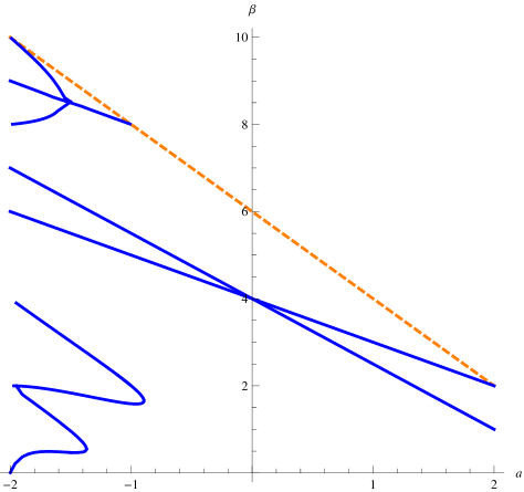
Figure 7: Blue solid curves: Locations in the $(a,\beta)$ plane, where $F(a,\beta)$ given in equation (198) vanishes. The two straight lines are given by $\beta_{1}=1+\frac{3}{2}(2-a)$ and $\beta_{2}=4-a$. Orange dashed line: $\beta=6-2a$.

Let us study the nonlinear term in the FRG equation for the SQG turbulence given by

$$J(k)=\int\frac{d^{2}{\bf q}}{(2\pi)^{2}}[{\bf q}\times{\bf k}]^{2}(q^{-a}-p^{-a})\tilde{\Delta}_{T}(q)\big{[}(q^{-a}-p^{-a})\tilde{\Delta}_{T}(p)-2(q^{-a}-k^{-a})\tilde{\Delta}_{T}(k)\big{]},$$ (191)

where ${\bf p}={\bf k}-{\bf q}$. We now assume for the correlator $\tilde{\Delta}_{T}(k)$ the form

$$\tilde{\Delta}_{T}(k)=\frac{1}{k^{\beta}}.$$ (192)

It is related to the velocity correlator $\Delta(k)$ by

$$\beta=4-2a+\zeta_{2},\ \quad,\quad\tilde{\Delta}(k)=\frac{1}{k^{2+\zeta_{2}}}.$$ (193)

Keeping in mind that the case $a=2$ corresponds to the NS equation in $N=2$, we expect that $\beta$ is close to $2$ near $a=2$. We thus want to compute

$$I(k):=\int\frac{\rmd^{2}{\bf q}}{(2\pi)^{2}}[{\bf q}\times{\bf k}]^{2}(q^{-a}-p^{-a})q^{-\beta}\big{[}(q^{-a}-p^{-a})p^{-\beta}-2(q^{-a}-k^{-a})k^{-\beta}\big{]}.$$ (194)

Using that

$$[{\bf q}\times{\bf k}]^{2}=k^{2}q^{2}-({\bf k}\cdot{\bf q})^{2}=-\frac{1}{4}\big{[}k^{4}-2k^{2}(q^{2}+({\bf k}-{\bf q})^{2})+(q^{2}-({\bf k}-{\bf q})^{2})^{2}\big{]}$$ (195)

we obtain

$$\!\!\!\!\!\!\!\!\!\!\!\!\!\!\!\!\!\!\!\!\!\!\!\!\!I(k)=-\frac{1}{4}\int_{t_{1},t_{2}>0}\Bigg{[}\frac{t_{1}^{a+\beta/2-1}t_{2}^{\beta/2-1}+t_{1}^{\beta/2-1}t_{2}^{a+\beta/2-1}}{\Gamma(a+\frac{\beta}{2})\Gamma(\frac{\beta}{2})}-2\frac{t_{1}^{a/2+\beta/2-1}t_{2}^{a/2+\beta/2-1}}{\Gamma(a/2+\frac{\beta}{2})^{2}}$$ (196)

$$~{}~{}~{}~{}~{}~{}~{}~{}~{}~{}~{}~{}~{}~{}-2k^{-\beta}\bigg{(}\frac{t_{1}^{a+\beta/2-1}}{\Gamma(a+\beta/2)}-k^{-a}\frac{t_{1}^{a/2+\beta/2-1}}{\Gamma(a/2+\beta/2)}\bigg{)}(-\partial_{t_{2}})+2k^{-\beta}\frac{t_{1}^{a/2+\beta/2-1}t_{2}^{a/2-1}}{\Gamma(a/2+\beta/2)\Gamma(a/2)}$$

$$~{}~{}~{}~{}~{}~{}~{}~{}~{}~{}~{}~{}~{}~{}-2k^{-a-\beta}\frac{t_{1}^{\beta/2-1}t_{2}^{a/2-1}}{\Gamma(\beta/2)\Gamma(a/2)}\Bigg{]}\tilde{B}(t_{1},t_{2})\int_{\bf q}e^{-t_{1}q^{2}-t_{2}({\bf k}-{\bf q})^{2}},$$

where $\tilde{B}(t_{1},t_{2})=k^{4}+2k^{2}(\partial_{t_{1}}+\partial_{t_{2}})+(\partial_{t_{1}}-\partial_{t_{2}})^{2}$. Using equation (183) for $N=2$ we find

$$I(k)=F(a,\beta)k^{-2(a+\beta-3)},$$ (197)

$$F(a,{\beta})=\frac{1}{32\pi}\Bigg{[}\Gamma(a+{\beta}-2)\left(\frac{8\Gamma\left(2-\frac{{\beta}}{2}\right)\Gamma\left(-a-\frac{{\beta}}{2}+2\right)}{\Gamma\left(\frac{{\beta}}{2}\right)\Gamma(-a-{\beta}+4)\Gamma\left(a+\frac{{\beta}}{2}\right)}-\frac{\sqrt{\pi}2^{a+{\beta}}\Gamma\left(-\frac{a}{2}-\frac{{\beta}}{2}+2\right)}{\Gamma\left(\frac{1}{2}(-a-{\beta}+5)\right)\Gamma\left(\frac{a+{\beta}}{2}\right)^{2}}\right)$$

$$~{}~{}~{}~{}~{}~{}~{}~{}~{}~{}~{}~{}~{}~{}~{}~{}~{}~{}~{}~{}+\frac{8\Gamma\left(2-\frac{a}{2}\right)\left(\frac{\Gamma\left(-\frac{a}{2}-\frac{{\beta}}{2}+2\right)\Gamma\left(a+\frac{{\beta}}{2}-2\right)}{\Gamma\left(-a-\frac{{\beta}}{2}+4\right)\Gamma\left(\frac{a+{\beta}}{2}\right)}+\frac{\Gamma\left(2-\frac{{\beta}}{2}\right)\Gamma\left(\frac{1}{2}(a+{\beta}-6)\right)}{\Gamma\left(\frac{{\beta}}{2}\right)\Gamma\left(-\frac{a}{2}-\frac{{\beta}}{2}+3\right)}\right)}{\Gamma\left(\frac{a}{2}\right)}\Bigg{]}.$$ (198)

One checks that for $a=2$ one recovers $C(N=2,\zeta_{2})=F(a=2,\beta=\zeta_{2})$ where $C(N,\zeta_{2})$ is given by equation (61). As we already know this means that the limits $\beta\to 2$ and $a\to 2$ are not exchangeable without an IR cutoff. Indeed, we have $\lim_{\beta\to 2}F(a=2,\beta)=-1/(4\pi)$ and not $-1/(8\pi)$, which we expect in the presence of an IR cutoff. However, we find that if one keeps $a\neq 2$ infinitesimally close to $2$, and then takes the limit $\beta\to 2,$ one does find $-1/(8\pi)$. This means that one needs to keep $a>2$, and that $\lim_{a\to 2}F(a,\beta=2)=-1/(8\pi)$ is the correct limit.

This result leaves two options for the large-$k$ behavior of possible fixed points parameterized by $\beta$:

(i) $\beta=6-2a$ leads to the nonlinear term in the FRG equation which for large $k$ asymptotics is also $\sim Fk^{-\beta}$. Thus, it can be balanced by the rescaling terms and may have a self consistent solution even if $F$ is not zero. The tail is then given by $\Delta_{T}(k)\sim 1/k^{6-2a}$. In this case the tail $\Delta(k)\sim 1/k^{4}$ for the velocity remains independent of $a$.

(ii) there is a value of $\beta<6-2a$ where $F(a,\beta)$ vanishes. All possible values are shown on figure 7 for $-2\leq a\leq 2$. For instance we find that $F(a,\beta)$ vanishes for $\beta_{1}=1+\frac{3}{2}(2-a)$ and $\beta_{2}=4-a$, which cross at $a=0$. However, there are other values.

If we ask that the function $\zeta_{2}(a)$ for the physical fixed point is continuous, it follows from our analysis for the 2D NS equation (where $\zeta_{2}(a=2)=2$) that likely values are $\zeta_{2}(a)=2$ or $\zeta_{2}(a)=a$ for $a>0$. However more work is clearly called for, in view of these results, to study possible fixed points as a function of $a$.

Appendix G Small-$k$ expansion for Navier-Stokes in dimension $N=2$

In this appendix, we calculate the small-$k$ expansion of the nonlinear term in the FRG equation for the 2-dimensional decaying Navier-Stokes turbulence. This will allow us to find in a self-consistent way the small-$k$ behavior of the FP solution $\tilde{\Delta}^{*}(k)$. To this aim, consider the non-linear contribution to the flow-equation in the distance geometry representation given by equation (71). It is useful to symmetrize it in $t\to-t$:

$$\delta\tilde{\Delta}(k)=\frac{k^{4}}{4\pi^{2}}\int_{1}^{\infty}\rmd s\int_{0}^{1}\rmd t\frac{st}{s^{2}-t^{2}}\sqrt{(s^{2}-1)(1-t^{2})}$$ (199)

$$\hphantom{\delta\tilde{\Delta}(k)=}\times\left\{\!\left[\Big{(}(s-t)^{2}-4\Big{)}\tilde{\Delta}\big{(}{\textstyle\frac{k}{2}}(s{-}t)\big{)}-\Big{(}(s+t)^{2}{-}4\Big{)}\tilde{\Delta}\big{(}{\textstyle\frac{k}{2}}(s{+}t)\big{)}\right]\!\tilde{\Delta}(k)+4{st}\tilde{\Delta}\big{(}{\textstyle\frac{k}{2}}(s{-}t)\big{)}\tilde{\Delta}\big{(}{\textstyle\frac{k}{2}}(s{+}t)\big{)}\!\right\}.\!$$

We now want to expand equation (199) in small $k$ for an arbitrary function $\tilde{\Delta}(k)$. In Sec. 6.2.2 we already discussed that the expected behavior of the fixed-point solution $\tilde{\Delta}^{*}(k)$ at small $k$ is $\tilde{\Delta}(k)\sim k^{n-1}$ with $n=3$. Let us for the moment consider a more general class of functions with a finite $\tilde{\Delta}(k=0)$ and $\tilde{\Delta}^{\prime}(k=0)$. It is not possible to expand the integrand of (199) in small $k$, since this gives integrals diverging at large $s$. Instead, one can rescale $s$, by defining $s=2q/k$, and only then expand in $k$. This allows one to integrate term by term over $t\in[0,1]$,

$$\delta\tilde{\Delta}(k)=-\frac{k^{2}}{8\pi}\int_{k/2}^{\infty}\rmd q\,\Big{[}q^{2}\tilde{\Delta}^{\prime}(q)\tilde{\Delta}(0)+2q\tilde{\Delta}(q)\big{(}\tilde{\Delta}(0)-\tilde{\Delta}(q\big{)}\Big{]}-\frac{k^{3}}{8\pi}\tilde{\Delta}^{\prime}(0)\int_{k/2}^{\infty}\rmd q\,\Big{[}2q\tilde{\Delta}(q)+q^{2}\Delta^{\prime}(q)\Big{]}+O(k^{4})$$

$$\hphantom{\delta\tilde{\Delta}(k)}=\frac{k^{2}}{4\pi}\int_{0}^{\infty}\rmd q\,q\tilde{\Delta}(q)^{2}+O(k^{4}).$$ (200)

We have used integrations by parts and the large-$k$ behavior (73) which suggests that $\lim_{k\to\infty}k^{2}\tilde{\Delta}(k)=0$. Note that the expansion of $\tilde{\Delta}(q)$ in the integrands of the first line of equation (200) can not produce terms of order $k^{4}$. Expanding (199) further to order $k^{4}$, we find

$$\delta\tilde{\Delta}(k)=...+\frac{k^{4}}{384\pi}\int_{k/2}^{\infty} \rmd q \Big{\{}6\tilde{\Delta}^{\prime}(q)\Big{[}7\tilde{\Delta}(0)-4q^{2}\tilde{\Delta}^{\prime\prime}(0)\Big{]}-12q\tilde{\Delta}^{\prime}(q)^{2}$$ (201)

$$-q\Big{[}12\tilde{\Delta}(q)\Big{(}4\tilde{\Delta}^{\prime\prime}(0)-\tilde{\Delta}^{\prime\prime}(q)\Big{)}+\tilde{\Delta}(0)\Big{(}q\tilde{\Delta}^{\prime\prime\prime}(q)+6\tilde{\Delta}^{\prime\prime}(q)\Big{)}\Big{]}\Big{\}}.$$

Together with (200), this yields

$$\delta\tilde{\Delta}(k)=\frac{k^{2}}{4\pi}\int_{0}^{\infty}\rmd q\,q\tilde{\Delta}(q)^{2}-\frac{k^{4}}{16\pi}\int_{0}^{\infty}\rmd q\,q\tilde{\Delta}^{\prime}(r)^{2}-\frac{5k^{4}}{48\pi}\tilde{\Delta}(q=0)^{2}+O(k^{5}).$$ (202)

Note that at least the first few terms of the expansion (202) depend mainly on the integral properties of $\tilde{\Delta}(k)$ and not on its small-$k$ expansion.

Appendix H Asymptotic large-$k$ behavior for Navier-Stokes in $N=2$

In this appendix, we calculate the asymptotic large-$k$ behavior of the non-linear term in the flow-equation for 2D Navier Stokes. We start from the rescaled dimensionless version of (26), setting

$$\tilde{\Delta}(k)\to\frac{1}{(k^{2}+m^{2})^{2}}.$$ (203)

Thus we need to compute for $N=2$ the convergent integral

$${\delta\tilde{\Delta}(k)}=2\int\frac{\rmd^{2}{\bf q}}{(2\pi)^{2}}\frac{k^{2}q^{2}-({\bf k}\cdot{\bf q})^{2}}{k^{2}q^{2}({\bf k}-{\bf q})^{2}}\left[(k^{2}-q^{2})\Big{(}({\bf k}-{\bf q})^{2}-q^{2}\Big{)}\right]\frac{1}{(q^{2}+m^{2})^{2}}\left[\frac{1}{(({\bf k}-{\bf q})^{2}+m^{2})^{2}}-\frac{1}{(k^{2}+m^{2})^{2}}\right].\$$ (204)

In polar coordinates this integral reads

$${\delta\tilde{\Delta}(k)} = \frac{2}{(2\pi)^{2}}\int\limits_{0}^{\infty}q\,\rmd q\int\limits_{0}^{2\pi}\rmd\phi\,\frac{1-\cos^{2}(\phi)}{k^{2}-2kq\cos(\phi)+q^{2}}\left(k^{2}-q^{2}\right)\left[k^{2}-2kq\cos(\phi)\right]\frac{1}{\left(m^{2}+q^{2}\right)^{2}}$$ (205)

$$\qquad\times\left[\frac{1}{\left(k^{2}-2kq\cos(\phi)+m^{2}+q^{2}\right)^{2}}-\frac{1}{\left(k^{2}+m^{2}\right)^{2}}\right].$$

After rescaling $q\to qk$ and $m\to m_{1}k$ it becomes

$${\delta\tilde{\Delta}(k)} = \frac{2}{k^{4}(2\pi)^{2}}\int\limits_{0}^{\infty}q\,\rmd q\int\limits_{0}^{2\pi}\rmd\phi\,\frac{1-\cos^{2}(\phi)}{1-2q\cos(\phi)+q^{2}}\left(1-q^{2}\right)\left[1-2q\cos(\phi)\right]\frac{1}{\left(m_{1}^{2}+q^{2}\right)^{2}}$$ (206)

$$\qquad\times\left[\frac{1}{\left(1-2q\cos(\phi)+m_{1}^{2}+q^{2}\right)^{2}}-\frac{1}{\left(1+m_{1}^{2}\right)^{2}}\right].$$

Changing variables to $t$ in such a way that $\cos(\phi)\to\frac{1-t^{2}}{t^{2}+1}$ and $\sin(\phi)\to\frac{2t}{t^{2}+1}$ with Jacobian $\frac{4}{t^{2}+1}$ we arrive at

$${\delta\tilde{\Delta}(k)} = \frac{8}{\pi^{2}k^{4}}\int\limits_{0}^{\infty}q^{2}\rmd q\int\limits_{0}^{\infty}t^{2}\rmd t\frac{\left(q^{2}-1\right)\left(qt^{2}+q+2t^{2}-2\right)\left(2q\left(t^{2}-1\right)+t^{2}+1\right)}{(m_{1}^{2}+q^{2})^{2}\left[q^{2}\left(t^{2}+1\right)+2q(t^{2}-1)+t^{2}+1\right]}$$ (207)

$$\qquad\times\frac{\left(t^{2}+1\right)(2m_{1}^{2}+q^{2}+2)+2q\left(t^{2}-1\right)}{\left(m_{1}^{2}+1\right)^{2}\left(t^{2}+1\right)^{3}\left[\left(t^{2}+1\right)(m_{1}^{2}+1+q^{2})+2q\left(t^{2}-1\right)\right]^{2}}.$$

The integral over $t$ has to be taken independently for $0<q<1$ and $1<q<\infty$ so that $\delta\tilde{\Delta}(k)=\delta_{1}\tilde{\Delta}(k)+\delta_{2}\tilde{\Delta}(k)$. Introducing $A=\sqrt{m_{1}^{2}+(q-1)^{2}}$ and $B=\sqrt{m_{1}^{2}+(q+1)^{2}}$ one can write these integrals in the following form

$$\delta_{1}\tilde{\Delta}(k) = \frac{1}{\pi k^{4}}\int\limits_{0}^{1}\rmd q\,\frac{(B-A)^{3}\left[\left(A^{2}-B^{2}\right)^{2}-16\right]\left[A^{4}-2A^{2}\left(B^{2}+4\right)+B^{4}-8B^{2}\right]^{-2}}{AB\left[(A-B)^{2}-4\right]^{2}(A+B)\left(A^{2}+B^{2}-2\right)^{2}}$$ (208)

$$\qquad\times\bigg{[}A^{8}-4A^{7}B+2A^{6}\left(2B^{2}-9\right)+4A^{5}B\left(B^{2}+7\right)-2A^{4}\left(5B^{4}+7B^{2}-48\right)$$

$$\qquad\quad~{}+2A^{2}\left(2B^{6}-7B^{4}+32B^{2}-64\right)-4AB\left(B^{6}-7B^{4}+32\right)$$

$$\qquad\quad~{}+4A^{3}B^{3}\left(B^{2}+2\right)+B^{2}\left(B^{2}-8\right)^{2}\left(B^{2}-2\right)\bigg{]}$$

and

$$\delta_{2}\tilde{\Delta}(k) = \frac{1}{\pi k^{4}}\int\limits_{1}^{\infty}\rmd q\,\frac{(B-A)\left[(A+B)^{2}-2\right]\left[\left(A^{2}-B^{2}\right)^{2}-16\right]}{AB(A+B-2)^{2}(A+B)(A+B+2)^{2}\left(A^{2}+B^{2}-2\right)^{2}}.$$ (209)

Integration over $q$ and combining both terms gives

$$\delta\tilde{\Delta}(k)=-\frac{1}{8\pi k^{4}}f(m/k)$$ (210)

with

$$f(x) = \frac{1}{x^{4}\left(x^{2}+1\right)^{2}}\bigg{\{}\left(6x^{4}+8x^{2}+2\right)\log\left(x^{2}+1\right)+2\left(2x^{4}+x^{2}\right)$$ (211)

$$+\sqrt{4x^{2}+1}\left(x^{2}+1\right)^{2}\bigg{[}\log\left(\sqrt{4x^{2}+1}-1\right)-\log\left(\left(x^{2}+1\right)\left(\sqrt{4x^{2}+1}+3\right)-2\right)\bigg{]}$$

$$+\left[\left(\sqrt{4x^{2}+1}-6\right)x^{2}+\sqrt{4x^{2}+1}-2\right]\left(x^{2}+1\right)\log\left(x^{2}\right)\bigg{\}}.$$

Expanding in small $x$, i.e. large $k/m$, we obtain

$$f(x)=1+x^{2}\left(8\log(x)-\frac{2}{3}\right)-x^{4}\left(32\log(x)+\frac{53}{6}\right)+O\left(x^{5}\right).$$ (212)

Note that only the leading term is universal, while the higher ones depend on the regularization by $m$ introduced in equation (203). This implies the leading-order term $-\frac{A^{2}}{8\pi k^{4}}$ given in equation (80).

Appendix I Numerical solution for the fixed point in dimension $N=2$

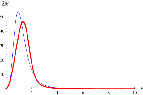
Figure 8: Left: Check for the precision of the fit for $f(t)$ defined in Eq. (214). Right: The guessed fixed-point $\tilde{\Delta}_{\mathrm{guess}}(k)$ (blue, thin line), and the numerical solution $\tilde{\Delta}(k)$ defined in Eq. (84) (red, fat line). See figure 2 for a log-log plot of $\tilde{\Delta}(k)$.

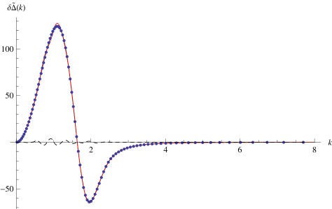
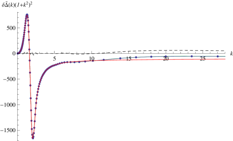
Figure 9: Top left: $\delta\tilde{\Delta}(k)$ (green solid line with superimposed blue dots), $2\tilde{\Delta}(k)+k\tilde{\Delta}^{\prime}(k)$ (solid red line) and $\partial_{\ell}\tilde{\Delta}(k)$ (dashed black line). Top right: The same 3 terms, multiplied by $(1+k^{2})^{2}$. Bottom: plot of the ratio $\frac{\delta\tilde{\Delta}(k)}{2\tilde{\Delta}(k)+k\tilde{\Delta}^{\prime}(k)}$ which must be 1 at the fixed point.

We wish to integrate equations (65) and (71) numerically, using $\zeta=2$. If the fixed point is attractive, $\tilde{\Delta}(k)$ will converge against it. Numerically, the problem is hard for several reasons:

1. convergence of the integral (71) for large $k$ is slow and imprecise.

2. one needs high precision for $\tilde{\Delta}(k)$, which respects the conditions (74) and (78) at small $k$, and the asymptotic form (80) for large $k$.

3. the r.h.s. of equation (65) must be calculated numerically at many different points; we will use 108 points (see table 1).

4. one easily runs into numerical instabilities, when using a spline-interpolation through all points, or a polynomial fit of degree $\approx 20$, which is necessary to represent faithfully the data-points.

In order to circumvent these problems, we do the following: Write the ansatz (84)-(85). The guess in equation (85) was obtained by (i) imposing the correct asymptotic forms, (ii) trying to optimize consistency relations as (202). Since we have no small-$k$ expansion with rapidly decaying coefficients, the final criterion (iii) for (85) was a r.h.s. in the flow-equation which is small in the intermediate regime of finite $k$.

Our information is stored in $\tilde{\Delta}_{\mathrm{cor}}(k)$, spaced as the first column in table 1. It is updated via

$$\tilde{\Delta}_{\mathrm{cor}}(k)\to\tilde{\Delta}_{\mathrm{cor}}(k)+\kappa\,t\partial_{t}\tilde{\Delta}(k)\ ,$$ (213)

at the given values of $k$. The quantity $\partial_{t}\tilde{\Delta}(k)$ is given by equations (65) and (71). Note that while we use the distance geometry formula (71) for the correction since it is numerically more efficient, we have checked that the result is the same when replacing equation (71) by equations (66) and (67). The step-size $\kappa$ is finally reduced to $\kappa=0.005$.

To circumvent the numerical problems mentioned under (4) above when obtaining the rescaling term in (65) and the numerical integral in (71), we approximate $\tilde{\Delta}_{\mathrm{cor}}(k)$ by the smooth function

$$\tilde{\Delta}_{\mathrm{cor}}(k)=\frac{f\big{(}t(k)\big{)}}{m(k)}$$ (214)

$$t(k):=\frac{k}{\sqrt{10+k^{2}}}$$ (215)

$$m(k):=\frac{\left(k^{2}+1\right)^{5/2}}{k^{2}}$$ (216)

The function $f(t)$ is defined on $[0,1]$, bounded (of order 100), and converges to 0 for $t$ to 0 or 1, see figure 8. In order to produce a smooth fit for $f(t)$, we use the best (i.e. least variance) cubic spline with $o$ equidistant points and $f(0)=f(1)=f^{\prime}(0)=f^{\prime}(1)=0$. $o$ is initially chosen to be 13, and then increased up to 20. Using splines of this relatively low order (compared with the number of data points) effectively filters out numerical noise. (Note: A polynomial fit of the same order is not adequate, but generates a dynamic instability. To further increase precision, a spline with variable switch-points could be used. $o=20$ is our upper limit due to RAM problems in the implementation of the integration routines, which split the integrals in pieces for each spline part.) Before updating $\tilde{\Delta}_{\mathrm{cor}}(k)$ via (213), the table of stored values for $\tilde{\Delta}_{\mathrm{cor}}(k)$ is replaced by the approximation (214). This is necessary for consistency. On the left of figure 8, we show our final result of the function $f(t)$, and the points from which it is constructed. One sees that no numerical artefact is present.

Our final result for $\tilde{\Delta}(k)$ is shown in a log-log plot on figure 2. A linear plot is presented on the right of figure 8 (fat red line), as well as our initial guess $\tilde{\Delta}_{\mathrm{guess}}(k)$. Note that since there exists a redundant mode (the choice of $k_{\rm max}$ at which $E(k)=k\tilde{\Delta}(k)$ is maximal, one could get these two curves closer. Numerical values for $\tilde{\Delta}(k)$ are given in table 1. The precision can be inferred from figure 9. It should be few percent (relative precision) for $k<5$, but the precision decreases for larger values of $k$. Note however that we know the exact asymptotic form $\tilde{\Delta}(k)=16\pi/k^{4}$.

$k$	$\tilde{\Delta}(k)$
0	0
0.0158116	0.0131526
0.0474395	0.117591
0.0790817	0.323878
0.110748	0.629261
0.142447	1.03318
0.174189	1.53977
0.205984	2.15575
0.237841	2.8848
0.26977	3.72542
0.301781	4.66717
0.333885	5.68728
0.366091	6.76818
0.39841	7.91167
0.430852	9.12235
0.463428	10.4041
0.496149	11.7583
0.529027	13.1873
0.562072	14.6963
0.595297	16.2907
0.628713	17.9758
0.662334	19.758
0.69617	21.6242
0.730237	23.5339
0.764546	25.447
0.799113	27.3277
0.83395	29.1463

$k$	$\tilde{\Delta}(k)$
0.869074	30.8943
0.9045	32.5893
0.940243	34.2548
0.976321	35.9175
1.01275	37.6048
1.04955	39.3028
1.08673	40.9413
1.12433	42.4538
1.16235	43.782
1.20082	44.876
1.23977	45.7066
1.2792	46.2688
1.31916	46.5628
1.35967	46.5915
1.40074	46.3608
1.44242	45.8577
1.48473	45.0426
1.5277	43.8845
1.57137	42.3626
1.61578	40.4659
1.66095	38.2213
1.70694	35.7034
1.75378	32.9836
1.80152	30.1263
1.85021	27.1889
1.8999	24.2391
1.95064	21.362

$k$	$\tilde{\Delta}(k)$
2.0025	18.629
2.05554	16.0965
2.10983	13.8072
2.16544	11.7798
2.22246	10.005
2.28096	8.46986
2.34104	7.15983
2.40281	6.05898
2.46637	5.14416
2.53185	4.38304
2.59937	3.74686
2.66909	3.21119
2.74115	2.7555
2.81574	2.36475
2.89304	2.02966
2.97328	1.74234
3.05668	1.49586
3.14352	1.28418
3.23409	1.10221
3.32872	0.945681
3.42779	0.810933
3.53174	0.694791
3.64104	0.59454
3.75626	0.507916
3.87803	0.433078
4.00711	0.368428
4.14436	0.312578

$k$	$\tilde{\Delta}(k)$
4.29082	0.264334
4.44768	0.222674
4.6164	0.186731
4.79873	0.15576
4.99681	0.12912
5.21327	0.106266
5.45142	0.0867232
5.71548	0.0700738
6.01089	0.0559517
6.34489	0.044037
6.72728	0.0340508
7.17178	0.0257567
7.69832	0.0189527
8.33709	0.0134578
9.13673	0.00910839
10.1818	0.00575792
11.6362	0.00328225
13.8756	0.00157192
16	0.000868729
18.0514	0.00052673
20	0.000344759
23.5	0.000177434
27	0.000100406
31.5	0.0000534954
35.5	0.0000328852
41	0.0000183294
48	9.68650 $\times 10^{-6}$

Table 1: Numerical fixed point of equations (65), (71) for $\tilde{\Delta}(k)$.

Appendix J Navier-Stokes equation in the limit of large $N$

In this appendix we consider the FRG flow for the Navier-Stokes equation (32) in the limit of large $N$. We start from the flow equation in real space (32) to derive an equation for $\nabla_{{\bf u}}^{2}\Delta(u)$:

$$t\partial_{t}\nabla_{{\bf u}}^{2}\tilde{\Delta}(u)=(2-\zeta)\,\nabla_{{\bf u}}^{2}\tilde{\Delta}(u)+\frac{\zeta}{2}{\bf u}\partial_{\bf u}\big{[}\nabla_{{\bf u}}^{2}\tilde{\Delta}(u)\big{]}+\nabla_{{\bf u}}^{2}\delta\tilde{\Delta}_{\rm L}(u)+\nabla_{{\bf u}}^{2}\delta\tilde{\Delta}_{\rm NL}(u).$$ (217)

The Laplacian is $\nabla_{{\bf u}}^{2}=N\rmd/\rmd y+2y\,\rm d^{2}/dy^{2}$; rewriting $\Delta(u)$ in terms of $r(y),$ given by equation (31), we obtain

$$\nabla_{{\bf u}}^{2}\Delta(u)=-\bigg{[}N\,\left(2+N\right)\,r^{\prime\prime}(y)+4\,y\,\left(\left(2+N\right)\,r^{\prime\prime\prime}(y)+y\,r^{(4)}(y)\right)\bigg{]}.$$ (218)

The Laplacian of $\nabla_{{\bf u}}^{2}\delta\tilde{\Delta}_{\rm L}(u)$ is local and has been expressed in terms of $r(y)$ in equation (33). The nonlocal part $\delta\tilde{\Delta}_{\rm NL}(u)$ is given by equation (34) with the kernel (35). Taking into account that for a large-$N$ expansion in real space, both $p^{2}$ and $k^{2}\sim N$, we can expand the kernel in $1/N$ as follows

$$A(p,k)=2k^{4}\left(1-\frac{1}{N}\right)-\frac{4}{N}\frac{k^{4}p^{2}}{k^{2}+p^{2}}+O\!\left(\frac{1}{N^{2}}\right)\ .$$ (219)

The first term in equation (219) can be written as a derivative, thus becomes also local

$$\nabla_{{\bf u}}^{2}\delta{\tilde{\Delta}_{\rm NL}^{(1)}(u)}=2\left(N-1\right)\,r^{\prime}(0)\left[\left(4+N\right)\left(\left(2+N\right)\left(N\,r^{\prime\prime\prime}(y)+6\,y\,r^{(4)}(y)\right)+12\,y^{2}\,r^{(5)}(y)\right)+8\,y^{3}\,r^{(6)}(y)\right].\ \ \ \$$ (220)

Note that apart from the factor of $r^{\prime}(0)$, it has the structure of the last term in equation (33). Let us now evaluate the second term in equation (219) to leading order at large $N$,

$$\nabla_{{\bf u}}^{2}\delta\tilde{\Delta}_{\rm NL}^{(2)}(u) = -\frac{{4}}{N}\int_{k,p}e^{-iku}k^{6}\tilde{R}(k)\frac{1}{k^{2}+p^{2}}p^{4}\tilde{R}(p)$$ (221)

$$= -\frac{{4}}{N}\int_{0}^{\infty}\rmd t\int_{k,p}e^{-iku}k^{6}\tilde{R}(k)p^{4}\tilde{R}(p)e^{-tk^{2}-tp^{2}}\ .$$

Since $\int_{k}e^{-iku}\tilde{R}(k)=\tilde{R}(u)=r(y),$ we have in the large-$N$ limit

$$\int_{k}e^{-iku}e^{-tk^{2}}{\tilde{R}(k)}=r(y+Nt)\ ,$$ (222)

as can be checked by Taylor expanding and using that $-k^{2}=\nabla_{{\bf u}}^{2}=N\rmd/\rmd y$ to leading order. Hence

$${\nabla_{{\bf u}}^{2}\delta\tilde{\Delta}_{\rm NL}^{(2)}(u)}=\frac{{4}}{N}N^{5}\int_{0}^{\infty}\rmd t\,r^{\prime\prime\prime}(y+Nt)r^{\prime\prime}(Nt)=\frac{{4}}{N}N^{4}\int_{0}^{\infty}\rmd z\,r^{\prime\prime\prime}(y+z)r^{\prime\prime}(z).$$ (223)

We now put all pieces together, setting $\zeta=\zeta_{0}+\zeta_{-1}/N+...$ Expanding to order $1/N$ we obtain equation (94).

References

Contents

References

- [1] A.N. Kolmogorov, On the energy distribution in the spectrum of a turbulent flow, C.R. Acad. Sci. URSS 30 (1941) 301–305.
- [2] A.N. Kolmogorov, A refinement of previous hypotheses concerning the local structure of turbulence in a viscous incompressible fluid at high reynolds number, J. Fluid Mech. 13 (1962) 82–85.
- [3] U. Frisch, Turbulence, Cambridge University Press, 1995.
- [4] A.M. Oboukhov, Some specific featues of atmoshperic turbulence, J. Fluid Mech. 13 (1962) 77–81.
- [5] R.H. Kraichnan, The structure of isotropic turbulence at very high reynolds numbers, Journal of Fluid Mechanics 5 (1959) 497–543.
- [6] M. Lesieur, Turbulence in Fluids, Kluwer Academic Publishers, Dordrecht/Boston/London, third edition, 1995.
- [7] C.-Y. Mou and P.B. Weichman, Spherical model for turbulence, Phys. Rev. Lett. 70 (1993) 1101–1104.
- [8] C.-Y. Mou and P.B. Weichman, Multicomponent turbulence, the spherical limit, and non-kolmogorov spectra, Phys. Rev. E 52 (1995) 3738–3796.
- [9] R.H. Kraichnan, Small-scale structure of a scalar field convected by turbulence, Phys. Fluids 11 (1968) 945–953.
- [10] D. Forster, D.R. Nelson and M.J. Stephen, Large-distance and long-time properties of a randomly stirred fluid, Phys. Rev. A 16 (1977) 732–749.
- [11] C. DeDominicis and P.C. Martin, Energy spectra of certain randomly-stirred fluids, Phys. Rev. A 19 (1979) 419–422.
- [12] J.R. Mayo, Field theory of the inverse cascade in two-dimensional turbulence, Phys. Rev. E 72 (2005) 056316.
- [13] L.T. Adzhemyan, N.V. Antonov, P.B. Gol’din, T.L. Kim and M.V. Kompaniets, Renormalization group in the infinite-dimensional turbulence: third-order results, J. Phys. A 41 (2008) 495002.
- [14] L.Ts. Adzhemyan, N.V. Antonov, M.V. Kompaniets and A.N. Vasil’ev, Renormalization-group approach to the stochastic navier-stokes equation: Two-loop approximation, Int. J. Mod. Phys. B 17 (2003) 2137–2170.
- [15] LTs. Adzhemyan, NV. Antonov and AN. Vasil’ev, Infrared divergences and the renormalization group in the theory of fully developed turbulence, Zhurnal Eksperimentalnoi i Teoreticheskoi Fiziki 95 (1989) 1272–8.
- [16] A.M. Polyakov, Turbulence without pressure, Phys. Rev. E 52 (1995) 6183–6188, hep-th/9506189.
- [17] S. Boldyrev, T. Linde and A. Polyakov, Velocity and velocity-difference distributions in Burgers turbulence, Phys. Rev. Lett. 93 (2004) 184503, nlin.CD/0305014.
- [18] A.M. Polyakov, The theory of turbulence in 2-dimensions, Nucl. Phys. B 396 (1993) 367–385, hep-th/9212145.
- [19] W. Pauls, T. Matsumoto, U. Frisch and J. Bec, Nature of complex singularities for the 2D Euler equation, Physica D 219 (2006) 40–59.
- [20] M. Chertkov, A. Pumir and B.I. Shraiman, Lagrangian tetrad dynamics and the phenomenology of turbulence, chao-dyn/9905027 (1999).
- [21] V.S. L’vov, E. Podivilov, A. Pomyalova, I. Procaccia and D. Vandembroucq, Improved shell model of turbulence, Phys. Rev. E 58 (1998) 1811–1822.
- [22] L. Ts. Adzhemyan, N.V. Antonov, J. Honkonen and T. L. Kim, Anomalous scaling of a passive scalar advected by the navier-stokes velocity field: Two-loop approximation, Phys. Rev. E 71 (2005) 016303.
- [23] M. Chertkov, G. Falkovich, I. Kolokolov and V. Lebedev, Normal and anomalous scaling of the fourth-order correlation function of a randomly advected passive scalar, Phys. Rev. E 52 (1995) 4924–4941.
- [24] K. Gawedzki and M. Vergassola, Phase transition in the passive scalar advection, Physica D 138 (2000) 63–90.
- [25] A.L. Fairhall, O. Gat, V. L‘vov and I. Procaccia, Anomalous scaling in a model of passive scalar advection: exact results, Phys. Rev. E 53 (1996) 3518–35.
- [26] G.L. Eyink and J. Xin, Self-similar decay in the Kraichnan model of a passive scalar, J. of Stat. Phys. 100 (2000) 679–741.
- [27] K. Gawȩdzki and M. Vergassola, Phase transition in the passive scalar advection, cond-mat/9811399 (1998).
- [28] V.S. L’vov, I. Procaccia and A.L. Fairhall, Anomalous scaling in fluid mechanics: the case of the passive scalar, Phys. Rev. E 50 (1994) 4684–704.
- [29] K.J. Wiese, The passive polymer problem, J. Stat. Phys. 101 (2000) 843–891, chao-dyn/9911005.
- [30] L.T. Adzhemyan and N.V. Antonov, Renormalization group and anomalous scaling in a simple model of passive scalar advection in compressible flow, Phys. Rev. E 58 (1998) 7381–96.
- [31] D. Bernard, K. Gawȩdzki and A. Kupiainen, Anomalous scaling in the n-point functions of a passive scalar, Phys. Rev. E 54 (1996) 2564–2572.
- [32] D. Bernard, K. Gawedzki and A. Kupiainen, Slow modes in passive advection, J. of Stat. Phys. 90 (1998) 519–69.
- [33] S. Chen and R.H. Kraichnan, Simulations of a randomly advected passive scalar field, Phys. Fluids 10 (1998) 2867–84.
- [34] M. Chertkov and G. Falkovich, Anomalous scaling of a white advected passive scalar, Phys. Rev. Lett. 76 (1996) 2706.
- [35] U. Frisch, A. Mazzino, A. Noullez and M. Vergassola, Lagrangian method for multiple correlations in passive scalar advection, Phys. Fluids 11 (1999) 2178–86.
- [36] K. Gawȩdzki and A. Kupiainen, Anomalous scaling of the passive scalar, Phys. Rev. Lett. 75 (1995) 3834.
- [37] R.H. Kraichnan, V. Yakhot and S. Chen, Scaling relations for a randomly advected passive scalar field, Phys. Rev. Lett. 75 (1995) 240–3.
- [38] G. Falkovich, K. Gawedzki and M. Vergassola, Particles and fields in fluid turbulence, Rev. Mod. Phys. 73 (2001) 913.
- [39] O. Gat, VS. L’vov, E. Podivilov and I. Procaccia, Nonperturbative zero modes in the Kraichnan model for turbulent advection, Phys. Rev. E 55 (1997) R3836–9.
- [40] B.I. Shraiman and E.D. Siggia, Symmetry and scaling of turbulent mixing, Phys. Rev. Lett. 77 (1996) 2463–6.
- [41] G.K. Batchelor, Computation of the energy spectrum in homogeneous two dimensional turbulence, Phys. Fluids 12 (1969) II–233.
- [42] D. Bernard, G. Boffetta, A. Celani and G. Falkovich, Inverse turbulent cascades and conformally invariant curves, Phys. Rev. Lett. 98 (2007) 024501.
- [43] M.A.I. Flohr, Two-dimensional turbulence: A novel approach via logarithmic conformal field theory, Nucl. Phys. B 482 (1996) 567 – 578.
- [44] C. Eling, I. Fouxon and Y. Oz, The incompressible Navier-Stokes equations from black hole membrane dynamics, Phys. Lett. B 680 (2009) 496–499.
- [45] I. Bredberg, A. Strominger Black Holes as Incompressible Fluids on the Sphere, arXiv:1106.3084.
- [46] I. Bredberg, C. Keeler, V. Lysov, A. Strominger From Navier-Stokes To Einstein arXiv:1101.2451
- [47] M. Müller, J. Schmalian and L. Fritz, Graphene: A nearly perfect fluid, Phys. Rev. Lett. 103 (2009) 025301.
- [48] J. Bec and K. Khanin, Burgers turbulence, Phys. Rep. 447 (2007) 1–66.
- [49] P. Le Doussal, Chaos and residual correlations in pinned disordered systems, Phys. Rev. Lett. 96 (2006), cond-mat/0505679.
- [50] U. Frisch and J. Bec, Burgulence, in New Trends in Turbulence, Springer EDP-Sciences, 2001.
- [51] J.P. Bouchaud, M. Mezard and G. Parisi, Scaling and intermittency in Burgers turbulence, Phys. Rev. E 52 (1995) 3656–3674, cond-mat/9503144.
- [52] M. Mezard, Disordered systems and Burger’s turbulence, J. Phys. IV (France) 8 (1997) 27–38.
- [53] P. Le Doussal, M. Müller and K.J. Wiese, Avalanches in mean-field models and the Barkhausen noise in spin-glasses, EPL 91 (2010) 57004, arXiv:1007.2069.
- [54] P. Le Doussal, M. Müller and K.J. Wiese, Cusps and shocks in the renormalized potential of glassy random manifolds: How functional renormalization group and replica symmetry breaking fit together, Phys. Rev. B 77 (2007) 064203, arXiv:0711.3929.
- [55] J.D. Fournier, U. Frisch and H.A. Rose, Infinite-dimensional turbulence, J. Phys. A 11 (1978) 187–198.
- [56] M. Hairer, Solving the KPZ equation, arXiv:1109.6811 (2011).
- [57] D.S. Fisher, Interface fluctuations in disordered systems: expansion, Phys. Rev. Lett. 56 (1986) 1964–97.
- [58] P. Le Doussal, K.J. Wiese and P. Chauve, Functional renormalization group and the field theory of disordered elastic systems, Phys. Rev. E 69 (2004) 026112, cond-mat/0304614.
- [59] K.J. Wiese and P. Le Doussal, Functional renormalization for disordered systems: Basic recipes and gourmet dishes, Markov Processes Relat. Fields 13 (2007) 777–818, cond-mat/0611346.
- [60] P. Le Doussal, Functional renormalisation for disordered systems, in Euro-Summer School on Condensed Matter Theory 2004, lecture notes at http://www.lancs.ac.uk/users/esqn/windsor04/program.htm.
- [61] P. Le Doussal, Finite temperature Functional RG, droplets and decaying Burgers turbulence, Europhys. Lett. 76 (2006) 457–463, cond-mat/0605490.
- [62] P. Le Doussal, Exact results and open questions in first principle functional RG, Annals of Physics 325 (2009) 49–150, arXiv:0809.1192.
- [63] L. Balents, J.P. Bouchaud and M. Mézard, The large scale energy landscape of randomly pinned objects, J. Phys. I (France) 6 (1996) 1007–20.
- [64] P. Le Doussal and K.J. Wiese, Size distributions of shocks and static avalanches from the functional renormalization group, Phys. Rev. E 79 (2009) 051106, arXiv:0812.1893.
- [65] P. Le Doussal and K.J. Wiese, First-principle derivation of static avalanche-size distribution, Phys. Rev. E 85 (2011) 061102, arXiv:1111.3172.
- [66] P. Le Doussal, A. Rosso and K.J. Wiese, Shock statistics in higher-dimensional Burgers turbulence, EPL 96 (2011) 14005, arXiv:1104.5048.
- [67] V.S. L’vov, R.A. Pasmanter, A. Pomyalov and I. Procaccia, Strong universality in forced and decaying turbulence in a shell model, Phys. Rev. E 67 (2003) 066310.
- [68] P. Le Doussal, What can disordered systems tell us about turbulence, in The Nature of Turbulence, KITP program 2011, http://online.kitp.ucsb.edu/online/turbulence11/ledoussal/
- [69] J. Leray, Etude de diverses équations intégrales nonlinéaires et de quelques problèmes que pose l’hydrodynamique, J. Math. Pure Appl. 12 (1934) 1–82.
- [70] J. Leray, On the movement of a viscous fluid to fill the space, Acta Mathematica 63 (1934) 193–248.
- [71] J. Duchon and R. Robert, Inertial energy dissipation for weak solutions of incompressible Euler and Navier-Stokes equations, Nonlinearity 13 (2000) 249–255.
- [72] K. Gawedzki, Easy turbulence, arXiv:chao-dyn/9907024 (1999).
- [73] S. Kida, Asymptotic properties of burgers turbulence, J. Fluid Mech. 93 (1979) 337–377.
- [74] J.-P. Bouchaud and M. Mézard, Universality classes for extreme-value statistics, J. Phys. A 30 (1997) 7997–8015, arXiv:cond-mat/9707047.
- [75] A. Rosso, Y.V. Fyodorov, P. Le Doussal, Freezing transition in decaying burgers turbulence and random matrix dualities, Europhys. Lett 90 (2010) 60004, arXiv:1004.5025.
- [76] S.N. Gurbatov, S.I. Simdyankin, E. Aurell, U. Frisch and G. Tóth, On the decay of burgers turbulence, J. Fluid Mech. 344 (1997) 339–374.
- [77] L. Balents and D.S. Fisher, Large- expansion of -dimensional oriented manifolds in random media, Phys. Rev. B 48 (1993) 5949–5963.
- [78] J.M. Burgers, The non-linear diffusion equation, Dordrecht, 1974.
- [79] T. de Karman and L. Howarth, On the statistical theory of isotropic turbulence, Proc. R. Soc. Lond. A 164 (1938) 192–215.
- [80] T. Shiromizu, Inverse cascade of primordial magnetic field in mhd turbulence, Phys. Lett. B 443 (1998) 127–130.
- [81] P. Schaeffer, On the dissipation rate coefficient in homogeneous isotropic decaying and forced turbulence, arXiv:1108.0575 (2011).
- [82] I. Proudman and W. H. Reid, On the decay of a normally distributed and homogeneous turbulent velocity field, Philosophical Transactions of the Royal Society of London. Series A, Mathematical and Physical Sciences (1954) 163–189.
- [83] G.L. Eyink and D.J. Thomson, Free decay of turbulence and breakdown of self-similarity, Physics of Fluids 12 (2000) 477.
- [84] P.D. Ditlevsen, M.H. Jensen and P. Olesen, Scaling and the prediction of energy spectra in decaying hydrodynamic turbulence, Physica A 342 (2004) 471–478.
- [85] G. Comte-Bellot and S. Corrsin, Simple Eulerian time correlation of full- and narrow-band velocity signals in grid-generated, “isotropic” turbulence, J. Fluid Mech. 48 (1971) 273 – 337.
- [86] Q. Chen, S. Chen and G.L. Eyink, The joint cascade of energy and helicity in three-dimensional turbulence, Phys. Fluids 15 (2003) 361.
- [87] D. Bernard and K. Gawedzki, Scaling and exotic regimes in decaying Burgers turbulence, J. Phys. A 31 (1998) 8735.
- [88] A.A. Fedorenko, P. Le Doussal and K.J. Wiese, in preparation.
- [89] P. Le Doussal and K.J. Wiese, 2-loop functional renormalization for elastic manifolds pinned by disorder in dimensions, Phys. Rev. E 72 (2005) 035101 (R), cond-mat/0501315.
- [90] G. Blatter, M.V. Feigel’man, V.B. Geshkenbein, A.I. Larkin and V.M. Vinokur, Vortices in high-temperature superconductors, Rev. Mod. Phys. 66 (1994) 1125.
- [91] T. Giamarchi and P. Le Doussal, Elastic theory of flux lattices in the presence of weak disorder, Phys. Rev. B 52 (1995) 1242–70.
- [92] L.D. Landau and E.M. Lifshitz, Fluid Mechanics, Volume 6, Pergamon Press, Oxford, 2 edition, 1987.
- [93] R.H. Kraichnan, Inertial-range transfer in 2-dimensional and 3-dimensional turbulence, J. Fluid Mech. 47 (1971) 525.
- [94] G. Falkovich and V. Lebedev, Universal direct cascade in 2-dimensional turbulence, Phys. Rev. E 50 (1994) 3883–3899.
- [95] J. Paret and P. Tabeling, Intermittency in the two-dimensional inverse cascade of energy: Experimental observations, Phys. Fluids 10 (1998) 3126–3136.
- [96] J. Paret, M.C. Jullien and P. Tabeling, Vorticity statistics in the two-dimensional enstrophy cascade, Phys. Rev. Lett. 83 (1999) 3418–3421.
- [97] C. Pasquero and G. Falkovich, Stationary spectrum of vorticity cascade in two-dimensional turbulence, Phys. Rev. E 65 (2002) 056305.
- [98] D. Bernard, Three-point velocity correlation functions in two-dimensional forced turbulence, Phys. Rev. E 60 (1999) 6184–6187, chao-dyn/9902010.
- [99] D. Bernard, Influence of friction on the direct cascade of the 2d forced turbulence, Europhys. Lett. 50 (2000) 333, chao-dyn/9904034.
- [100] G.L. Eyink, Dissipation in turbulent solutions of 2D Euler equations, Nonlinearity 14 (2001) 787–802.
- [101] P. Constantin, On the Euler equation of incompressible fluids, Bulletin (new series) of the American Mathematical Society 44 (2007) 603–621.
- [102] P. Constantin and F. Ramos, Inviscid limit for damped and driven incompressible Navier-Stokes equations in , Communications in Mathematical Physics 275 (2007) 529–551, arXiv:math/0611782.
- [103] P. Le Doussal and K.J. Wiese, Derivation of the functional renormalization group -function at order for manifolds pinned by disorder, Nucl. Phys. B 701 (2004) 409–480, cond-mat/0406297.
- [104] P. Le Doussal and K.J. Wiese, Functional renormalization group at large for disordered elastic systems, and relation to replica symmetry breaking, Phys. Rev. B 68 (2003) 174202, cond-mat/0305634.
- [105] P. Le Doussal and K.J. Wiese, Functional renormalization group at large for random manifolds, Phys. Rev. Lett. 89 (2002) 125702, cond-mat/0109204v1.
- [106] G. Boffetta, F. De Lillo and S. Musacchio, Inverse cascade in Charney-Hasegawa-Mima turbulence, Europhys. Lett. 59 (2002) 687–693, nlin/0203044.
- [107] G. Falkovich and S. Musacchio, Conformal invariance in inverse turbulent cascades, arXiv:1012.3868 (2012).
- [108] F. David, B. Duplantier and E. Guitter, Renormalization theory for interacting crumpled manifolds, Nucl. Phys. B 394 (1993) 555–664.