QCD resummation for semi-inclusive hadron production processes

Abstract

We investigate the resummation of large logarithmic perturbative corrections to hadron production in electron-positron annihilation and semi-inclusive deep-inelastic scattering. We find modest, but significant, enhancements of hadron multiplicities in the kinematic regimes accessible in present high-precision experiments. Our results are therefore relevant for the determination of hadron fragmentation functions from data for these processes.

I Introduction

Processes with identified final-state hadrons play important roles in QCD. Foremost, they provide crucial information on fragmentation functions and hence, ultimately, the hadronization mechanism. Modern analyses defloriandss ; strat ; akk ; hkns of fragmentation functions variously use data for single-inclusive annihilation (SIA) $e^{+}e^{-}\to hX$, semi-inclusive deep-inelastic scattering (SIDIS), $\ell p\to\ell hX$, and $pp\to hX$, where $h$ denotes a final-state hadron. Hadron production observables also serve as powerful probes of nucleon or nuclear structure. In particular, SIDIS measurements with polarized beams and/or targets have by now become indispensable tools for investigations of the spin structure of the nucleon in terms of helicity parton distribution functions and transverse-momentum dependent distributions Nowak . Finally, hadron production data also test some of our key concepts in the theoretical analysis of QCD at high energies, among them factorization, universality, and perturbative calculations.

In the present paper, we address higher-order perturbative corrections to two of the key hadron production processes, SIA $e^{+}e^{-}\to hX$ and SIDIS $\ell p\to\ell hX$. Our study is very much motivated by the recent advent of data for these reactions with unprecedented high precision. The BELLE collaboration at KEK has presented preliminary data belle for pion and kaon multiplicities in SIA that extend over a wide range in values of the fragmentation variable $x_{E}=2E^{h}/\sqrt{s}$, where $E^{h}$ is the energy of the produced hadron in the $e^{+}e^{-}$ center-of-mass system, and $\sqrt{s}=10.52$ GeV the collision energy. The BELLE data cover the region $0.2\leq x_{E}\leq 0.97$, with a very fine binning and extremely high precision partly at the sub-1% level. New preliminary high-statistics SIDIS data have been shown by the HERMES hermes and COMPASS compass collaborations over the past year or so.

In the kinematic regimes accessed by these experiments, perturbative-QCD corrections are expected to be fairly significant. In case of $e^{+}e^{-}\to hX$ at BELLE, as $x_{E}$ increases toward unity, the phase space for real-gluon radiation is very restricted, since most of the initial leptonic energy is used to produce the observed hadron and a recoiling unobserved final state. When this happens, the infrared cancellations between virtual and real-emission diagrams leave behind large logarithmic higher-order corrections to the basic $e^{+}e^{-}\to q\bar{q}$ cross section. These logarithms are very similar in nature to the “threshold logarithms” encountered in hadronic scattering processes when the energy of initial partons is just large enough to produce a given final state. Near $x_{E}=1$, it then becomes necessary to take the large corrections into account to all orders in the strong coupling, a technique known as threshold resummation. The SIDIS measurements, on the other hand, are characterized by two scaling variables, Bjorken-$x$ and a variable $z$ given by the energy of the produced hadron over the energy of the virtual photon in the target rest frame. The cross section is typically defined to be differential in both. Large logarithmic corrections to the SIDIS cross section arise when either one of the corresponding partonic variables becomes large. The most important effects arise when both are large, which is typically the case for the presently relevant fixed-target kinematics. As we shall discuss, in this case the logarithmic terms can be simultaneously resummed to all orders within the threshold resummation framework.

Previous work Sterman:2006hu has established a close correspondence between threshold resummation for the Drell-Yan process, double-inclusive annihilation $e^{+}e^{-}\to h_{1}h_{2}X$, and a variant of SIDIS for which one considers the cross section differential in the product $xz$ of the two scaling variables mentioned above, rather than in each of them separately. For this set of observables, the structure of the threshold logarithms turns out to be identical, up to trivial differences in the hard scattering functions that multiply the logarithms. One therefore can derive the resummation for each of the processes in the same manner, using exponentiation of eikonal diagrams in color-singlet processes webs ; LSV . This approach was termed crossed threshold resummation in Sterman:2006hu and will be the framework for our present analysis of SIDIS.

Resummation for $e^{+}e^{-}\to hX$ was addressed in detail in Refs. Cacciari:2001cw ; Blum ; Vogt ; Procura:2011aq . In Cacciari:2001cw the next-to-leading logarithm (NLL) expressions were presented, while extensions to next-to-next-to-leading logarithm and even next-to-next-to-next-to-leading logarithm were provided in Refs. Blum and Vogt , respectively. The global analysis of fragmentation functions of Ref. akk in fact includes NLL threshold resummation effects for $e^{+}e^{-}\to hX$ for the lower-energy data. They are found to improve the theoretical description and the quality of the fit to the data. Given the very high precision of the new BELLE data, a new phenomenological analysis of resummation effects is now timely and will be presented in this work. For now, we will restrict ourselves to resummation at NLL, which captures the main effects. As for SIDIS, an expression for the NLL resummed cross section was stated in Cacciari:2001cw , which turns out to be analogous to the related expressions for the rapidity-differential Drell-Yan cross section in terms of double-Mellin moments (see also Cat ; Bozzi:2007pn ). Phenomenological studies of resummation effects in SIDIS have never really been presented in the literature, except briefly in Vogelsang:2005tc . In the present paper, we derive the NLL resummed expression for SIDIS, making use of the techniques of Sterman:2006hu . We also present numerical results as relevant for comparisons to the recent SIDIS data.

Sections II and III collect our technical derivations. Since the resummation for SIDIS is the main new result, we mostly focus on this process and only briefly review the well-known results for $e^{+}e^{-}\to hX$ and inclusive deep-inelastic scattering (DIS). Section IV presents our phenomenological results.

II Resummation for SIDIS multiplicities

We consider semi-inclusive deep-inelastic scattering, $\ell(k)p(P)\to\ell(k^{\prime})h(P_{h})X$, where we have indicated the momenta of the involved particles. The momentum $q$ of the highly virtual photon exchanged between the incoming electron and proton is given by $q=k-k^{\prime}$. We define the usual variables

$$Q^{2} \equiv -q^{2}=-(k-k^{\prime})^{2},$$

$$x \equiv \frac{Q^{2}}{2P\cdot q},$$

$$y \equiv \frac{P\cdot q}{P\cdot k},$$

$$z \equiv \frac{P\cdot P_{h}}{P\cdot q}.$$ (1)

We have $Q^{2}=xys$, with $\sqrt{s}$ the $\ell p$ center-of-mass energy. In the current fragmentation region that we will consider here, the SIDIS cross section may be written as altarelli ; Nason:1993xx ; fupe ; graudenz ; deFlorian:1997zj ; roth :

$$\frac{d^{3}\sigma^{h}}{dxdydz} = \frac{4\,\pi\alpha^{2}}{Q^{2}}\left[\frac{1+(1-y)^{2}}{2y}{\cal F}_{T}^{h}(x,z,Q^{2})\right.$$ (2)

$$\hskip 31.2982pt\left.+\frac{1-y}{y}{\cal F}_{L}^{h}(x,z,Q^{2})\right],$$

where $\alpha$ is the fine structure constant. ${\cal F}_{T}^{h}$ and ${\cal F}_{L}^{h}$ are the transverse and the longitudinal structure functions; they are related to the more customary structure functions $F_{1}^{h}$ and $F_{L}^{h}$ by ${\cal F}_{T}^{h}\equiv 2F_{1}^{h}$ and ${\cal F}_{L}^{h}\equiv F_{L}^{h}/x$.

SIDIS hadron multiplicities are defined by

$$R^{h}_{\mathrm{SIDIS}}\equiv\frac{d^{3}\sigma^{h}/dxdydz}{d^{2}\sigma/dxdy},$$ (3)

where $d^{2}\sigma/dxdy$ is the cross section for inclusive DIS, $\ell p\to\ell X$, given by

$$\frac{d^{2}\sigma}{dxdy}=\frac{4\,\pi\alpha^{2}}{Q^{2}}\left[\frac{1+(1-y)^{2}}{2y}{\cal F}_{T}(x,Q^{2})+\frac{1-y}{y}{\cal F}_{L}(x,Q^{2})\right].$$ (4)

Here ${\cal F}_{T}\equiv 2F_{1}$ and ${\cal F}_{L}\equiv F_{L}/x$, with the standard inclusive structure functions $F_{1},F_{L}$. Usually, the numerator and denominator of (3) are averaged over suitable bins in $x$ and $y$. In order to investigate higher-order effects on SIDIS multiplicities, we have to consider QCD corrections to both the SIDIS and the inclusive DIS cross section. Since the latter has been treated very extensively in the literature, we will focus here on $d^{3}\sigma^{h}/dxdydz$ and only briefly summarize some of the known results for $d^{2}\sigma/dxdy$.

II.1 SIDIS cross section at next-to-leading order, and Mellin moments

Using factorization, the transverse and longitudinal structure functions ${\cal F}_{T}^{h}\equiv 2F_{1}^{h}$ and ${\cal F}_{L}^{h}\equiv F_{L}^{h}/x$ in (2) are given by ($i=T,L$)

$${\cal F}_{i}^{h}(x,z,Q^{2}) = \sum_{f,f^{\prime}}\int_{x}^{1}\frac{d\hat{x}}{\hat{x}}\int_{z}^{1}\frac{d\hat{z}}{\hat{z}}f\left(\frac{x}{\hat{x}},\mu^{2}\right)D^{h}_{f^{\prime}}\left(\frac{z}{\hat{z}},\mu^{2}\right)\,$$ (5)

$$\times\,{\cal{C}}^{i}_{f^{\prime}f}\left(\hat{x},\hat{z},\frac{Q^{2}}{\mu^{2}},\alpha_{s}(\mu^{2})\right),$$

where $f(\xi,\mu^{2})$ denotes the distribution of parton $f=q,\bar{q},g$ in the nucleon at momentum fraction $\xi$ and scale $\mu$, while $D^{h}_{f^{\prime}}\left(\zeta,\mu^{2}\right)$ is the corresponding fragmentation function for parton $f^{\prime}$ going to the observed hadron $h$. For simplicity, we have set all factorization and renormalization scales equal and collectively denoted them by $\mu$. The hard-scattering coefficient functions ${\cal{C}}^{i}_{f^{\prime}f}$ can be computed in perturbation theory:

$${\cal{C}}^{i}_{f^{\prime}f}\,=\,C^{i,(0)}_{f^{\prime}f}+\frac{\alpha_{s}(\mu^{2})}{2\pi}C^{i,(1)}_{f^{\prime}f}+{\cal O}(\alpha_{s}^{2}),$$ (6)

where, again, $i=T,L$. To lowest order (LO), only the process $\gamma^{*}q\to q$ contributes, and we have

$$C^{T,(0)}_{qq}(\hat{x},\hat{z}) = e_{q}^{2}\,\delta(1-\hat{x})\delta(1-\hat{z}),$$

$$C^{L,(0)}_{qq}(\hat{x},\hat{z}) = 0,$$ (7)

with the quark’s fractional charge $e_{q}$. Beyond LO, also gluons in the initial or final state contribute. The full set of the first-order coefficient functions altarelli ; Nason:1993xx ; fupe ; graudenz ; deFlorian:1997zj ; roth $C^{i,(1)}_{f^{\prime}f}$ are collected in the Appendix.

Since threshold resummation can be derived in Mellin-moment space, it is useful to take Mellin moments of the structure functions ${\cal F}_{T}^{h}$ and ${\cal F}_{L}^{h}$. Since $x$ and $z$ are independent variables, we take moments separately in both altarelli ; Stratmann:2001pb . We define

$$\tilde{{\cal F}}^{h}_{i}(N,M,Q^{2})\equiv\int_{0}^{1}dxx^{N-1}\int_{0}^{1}dzz^{M-1}\,{\cal F}^{h}_{i}(x,z,Q^{2}).$$ (8)

We then readily find from (5)

$$\tilde{{\cal F}}^{h}_{i}(N,M,Q^{2}) = \sum_{f,f^{\prime}}\tilde{f}^{N}(\mu^{2})\tilde{D}_{f^{\prime}}^{h,M}(\mu^{2})$$ (9)

$$\times\tilde{{\cal C}}^{i}_{f^{\prime}f}\left(N,M,\frac{Q^{2}}{\mu^{2}},\alpha_{s}(\mu^{2})\right),$$

where

$$\tilde{f}^{N}(\mu^{2})\equiv\int_{0}^{1}dxx^{N-1}f(x,\mu^{2}),$$

$$\tilde{D}_{f^{\prime}}^{h,M}(\mu^{2})\equiv\int_{0}^{1}dzz^{M-1}D^{h}_{f^{\prime}}(z,\mu^{2}),$$

$$\tilde{{\cal C}}^{i}_{f^{\prime}f}\left(N,M,\frac{Q^{2}}{\mu^{2}},\alpha_{s}(\mu^{2})\right)$$

$$\hskip 14.22636pt\equiv\int_{0}^{1}d\hat{x}\hat{x}^{N-1}\int_{0}^{1}d\hat{z}\hat{z}^{M-1}\,{\cal{C}}^{i}_{f^{\prime}f}\left(\hat{x},\hat{z},\frac{Q^{2}}{\mu^{2}},\alpha_{s}(\mu^{2})\right).$$

Thus, the Mellin moments of the structure functions are obtained from ordinary products of the moments of the parton distribution functions and fragmentation functions, and double-Mellin moments of the partonic hard-scattering functions. For the perturbative expansion given in (6), we have for the latter in lowest oder according to (II.1):

$$\tilde{C}^{T,(0)}_{qq}(N,M) = e_{q}^{2},$$

$$\tilde{C}^{L,(0)}_{qq}(N,M) = 0.$$ (11)

The corresponding moments of the next-to-leading order (NLO) terms $C^{i,(1)}_{f^{\prime}f}$ Stratmann:2001pb are also provided in the Appendix.

II.2 Resummation of the SIDIS coefficient function

As one can see from Eq. (49), the NLO coefficient function $C_{qq}^{T,(1)}(\hat{x},\hat{z})$ receives large corrections near $\hat{x},\hat{z}\to 1$. Choosing for simplicity $\mu_{F}=Q$, we have

$$C_{qq}^{T,(1)}(\hat{x},\hat{z}) \sim e_{q}^{2}C_{F}\Bigg{[}-8\delta(1-\hat{x})\delta(1-\hat{z})$$ (12)

$$+2\delta(1-\hat{x})\left(\frac{\ln(1-\hat{z})}{1-\hat{z}}\right)_{+}+2\delta(1-\hat{z})\left(\frac{\ln(1-\hat{x})}{1-\hat{x}}\right)_{+}$$

$$+\frac{2}{(1-\hat{x})_{+}(1-\hat{z})_{+}}\Bigg{]},$$

corresponding in moment space to

$$\tilde{C}_{qq}^{T,(1)}(N,M) \sim e_{q}^{2}C_{F}\Bigg{[}-8+\frac{\pi^{2}}{3}+\left(\ln\bar{N}+\ln\bar{M}\right)^{2}\Bigg{]},$$

where $\bar{N}\equiv N{\mathrm{e}}^{\gamma_{E}}$, $\bar{M}\equiv M{\mathrm{e}}^{\gamma_{E}}$, with $\gamma_{E}$ the Euler constant. Here we have only kept contributions that are neither suppressed as $1/N$, nor as $1/M$ in moment space. The terms given in (12) therefore always contain two distributions, one in $\hat{x}$ and one in $\hat{z}$.

Threshold resummation addresses the logarithms in $\bar{N}$ and $\bar{M}$ to all orders in the strong coupling constant $\alpha_{s}$. More precisely, it captures terms of the form $\alpha_{s}^{k}\ln^{n}N\ln^{m}M$, with $n+m\leq 2k$. We now discuss the derivation of the resummed expression for the SIDIS coefficient function $\tilde{C}_{qq}^{T,(1)}(N,M)$. Since the leading-order process is $\gamma^{*}q\to q$ scattering, and since both the incoming and the outgoing quark are “observed”, the treatment has much in common with that for the total Drell-Yan cross section, or for its “crossed” versions considered in Ref. Sterman:2006hu . A significant difference is, however, that in the present case two independent Mellin moments, $N$ and $M$, have to be considered. At large $N$ and $M$, or equivalently $\hat{x}$ and $\hat{z}$, all gluon radiation from the basic process $\gamma^{*}q\to q$ becomes soft, since we have the relation Sterman:2006hu

$$(1-\hat{x})+(1-\hat{z})\approx\frac{2k^{0}}{Q},$$ (14)

where $k^{0}$ is the total energy of gluon radiation. The coefficient function may then be evaluated in the eikonal approximation for the quarks and/or antiquarks involved in the hard scattering. In moment space, the eikonal hard scattering functions exponentiate, leading to Sterman:2006hu ; LSV ; webs

$$\tilde{\cal{C}}^{T,{\mathrm{res}}}_{qq}(N,M,\alpha_{s}(Q^{2})) \propto \exp\Bigg{[}\int_{0}^{Q^{2}}{dk_{\perp}^{2}\over k_{\perp}^{2}}A_{q}\left(\alpha_{s}(k_{\perp}^{2})\right)\Bigg{\{}\int_{\frac{k_{\perp}^{2}}{Q^{2}}}^{1}\frac{d\xi}{\xi}\left[{\mathrm{e}}^{-N\xi-M\frac{k_{\perp}^{2}}{\xi Q^{2}}}-1\right]+\ln\bar{N}+\ln\bar{M}\Bigg{\}}\Bigg{]},$$

which is valid to next-to-leading logarithmic (NLL) accuracy. Here, $A_{q}(\alpha_{s})$ is a perturbative function:

$$A_{q}(\alpha_{s})=\frac{\alpha_{s}}{\pi}A_{q}^{(1)}+\left(\frac{\alpha_{s}}{\pi}\right)^{2}A_{q}^{(2)}+\dots,$$ (16)

with

$$A_{q}^{(1)}=C_{F},\quad A_{q}^{(2)}=\frac{1}{2}C_{F}\left[C_{A}\left(\frac{67}{18}-\frac{\pi^{2}}{6}\right)-\frac{5}{9}N_{f}\right],$$ (17)

where $C_{F}=4/3$, $C_{A}=3$ and $N_{f}$ is the number of active flavors.

Up to corrections that are exponentially suppressed at large $N,M$, the integral over $\xi$ in (LABEL:nextA2) can be carried out analytically, and one finds

$$\int_{\frac{k_{\perp}^{2}}{Q^{2}}}^{1}\frac{d\xi}{\xi}\left[{\mathrm{e}}^{-N\xi-M\frac{k_{\perp}^{2}}{\xi Q^{2}}}-1\right]+\ln\bar{N}+\ln\bar{M}$$ (18)

$$\approx 2\left[K_{0}\left(\sqrt{NM}\,\frac{2k_{\perp}}{Q}\right)+\ln\left(\frac{k_{\perp}}{Q}\sqrt{\bar{N}\bar{M}}\right)\right],$$

where $K_{0}$ is a Bessel function. It arises when we extend the $\xi$ integral to $0<\xi<\infty$. It is instructive to confront this with the analogous expression for the Mellin-$N$ moments of the partonic total Drell-Yan cross section, which reads LSV ; Sterman:2006hu :

$$\int_{\frac{k_{\perp}^{2}}{Q^{2}}}^{1}\frac{d\xi}{\xi}\left[{\mathrm{e}}^{-N\left(\xi-\frac{k_{\perp}^{2}}{\xi Q^{2}}\right)}-1\right]+2\ln\bar{N}$$ (19)

$$\approx 2\left[K_{0}\left(N\,\frac{2k_{\perp}}{Q}\right)+\ln\left(\frac{k_{\perp}}{Q}\bar{N}\right)\right].$$

From this comparison one can immediately see that the result for the resummed SIDIS cross section can be obtained from the one for the total Drell-Yan cross section by simply setting $\bar{N}\to\sqrt{\bar{N}\bar{M}}$. In the case of SIDIS, the moments $N$ and $M$ independently fix the light-cone plus component $\xi$ and the minus component $\zeta=k_{\perp}^{2}/(\xi Q^{2})$ of the soft gluon momentum, resulting in the slightly more elaborate form of the exponent in (18). Likewise, the $\overline{\mathrm{MS}}$-subtraction of collinear divergencies in the initial and the final state in SIDIS yields the terms $\ln\bar{N}$ and $\ln\bar{M}$, respectively, whereas in Drell-Yan one has the contribution $2\ln\bar{N}$ from the two initial partons.

With (18), the final resummed coefficient function becomes in the $\overline{\mathrm{MS}}$ scheme:

$$\tilde{\cal{C}}^{T,{\mathrm{res}}}_{qq}(N,M,\alpha_{s}(Q^{2}))=e_{q}^{2}H_{qq}\left(\alpha_{s}(Q^{2}),\frac{Q^{2}}{\mu^{2}}\right)\exp\left[2\int_{0}^{Q^{2}}{dk_{\perp}^{2}\over k_{\perp}^{2}}A_{q}\left(\alpha_{s}(k_{\perp}^{2})\right)\left\{K_{0}\left(\sqrt{NM}\,\frac{2k_{\perp}}{Q}\right)+\ln\left(\frac{k_{\perp}}{Q}\sqrt{\bar{N}\bar{M}}\right)\right\}\right].$$ (20)

Here we have included a perturbative function $H_{qq}$ that collects the hard virtual corrections to $\gamma^{*}q\to q$ scattering. For resummation at NLL, one needs to know $H_{qq}$ to first order in the strong coupling, which may be derived by expanding (20) to ${\cal O}(\alpha_{s})$ (keeping only logarithmic terms in the exponent) and comparing to the explicit NLO expression (II.2) for large $N,M$. One finds:

$$H_{qq}\left(\alpha_{s},\frac{Q^{2}}{\mu^{2}}\right)=1+\frac{\alpha_{s}}{2\pi}C_{F}\left(-8+\frac{\pi^{2}}{3}+3\ln\frac{Q^{2}}{\mu^{2}}\right)+{\cal O}(\alpha_{s}^{2})\;.$$ (21)

We note that an alternative, but equivalent, form of the resummed result is Cat ; Cacciari:2001cw

$$\tilde{\cal{C}}^{T,{\mathrm{res}}}_{qq}(N,M,\alpha_{s}(Q^{2})) = e_{q}^{2}H_{qq}\left(\alpha_{s}(Q^{2}),\frac{Q^{2}}{\mu^{2}}\right)$$

$$\times\exp\left[\int_{0}^{1}dx\frac{\xi^{N}-1}{1-\xi}\int_{Q^{2}}^{(1-\xi)Q^{2}}\frac{dk_{\perp}^{2}}{k_{\perp}^{2}}A_{q}(\alpha_{s}(k_{\perp}^{2}))\right.$$

$$+\int_{0}^{1}d\zeta\frac{\zeta^{M}-1}{1-\zeta}\int_{Q^{2}}^{(1-\zeta)Q^{2}}\frac{dk_{\perp}^{2}}{k_{\perp}^{2}}A_{q}(\alpha_{s}(k_{\perp}^{2}))$$

$$\left.+\int_{0}^{1}dx\frac{\xi^{N}-1}{1-\xi}\int_{0}^{1}d\zeta\frac{\zeta^{M}-1}{1-\zeta}A_{q}\left(\alpha_{s}(Q^{2}(1-\xi)(1-\zeta))\right)\right].$$

This expression can be obtained from (LABEL:nextA2) by first writing the integrand as

$${\mathrm{e}}^{-N\xi-M\frac{k_{\perp}^{2}}{\xi Q^{2}}}-1 = \left({\mathrm{e}}^{-N\xi}-1\right)\left({\mathrm{e}}^{-M\frac{k_{\perp}^{2}}{\xi Q^{2}}}-1\right)$$ (23)

$$+{\mathrm{e}}^{-N\xi}-1+{\mathrm{e}}^{-M\frac{k_{\perp}^{2}}{\xi Q^{2}}}-1.$$

Including the integrals over $\xi$ and $k_{\perp}$ and substituting $k_{\perp}^{2}=\zeta\xi Q^{2}$, the first term on the right-hand-side of (23) yields

$$\int_{0}^{1}\frac{d\xi}{\xi}\left({\mathrm{e}}^{-N\xi}-1\right)\int_{0}^{1}\frac{d\zeta}{\zeta}\left({\mathrm{e}}^{-M\zeta}-1\right)A_{q}\left(\alpha_{s}(\zeta\xi Q^{2})\right).$$ (24)

Next, we deal with the term containing $\left({\mathrm{e}}^{-N\xi}-1\right)$ in (23). Combining with the logarithm $\ln\bar{N}$ in (LABEL:nextA2) we find, up to corrections suppressed as $1/N$:

$$\int_{0}^{Q^{2}}{dk_{\perp}^{2}\over k_{\perp}^{2}}A_{q}\left(\alpha_{s}(k_{\perp}^{2})\right)\left\{\int_{\frac{k_{\perp}^{2}}{Q^{2}}}^{1}\frac{d\xi}{\xi}\left({\mathrm{e}}^{-N\xi}-1\right)+\ln\bar{N}\right\}$$

$$\approx\int_{0}^{1}\frac{d\xi}{\xi}\left({\mathrm{e}}^{-N\xi}-1\right)\int_{Q^{2}}^{\xi Q^{2}}\frac{dk_{\perp}^{2}}{k_{\perp}^{2}}A_{q}\left(\alpha_{s}(k_{\perp}^{2})\right).$$ (25)

Likewise,

$$\int_{0}^{Q^{2}}{dk_{\perp}^{2}\over k_{\perp}^{2}}A_{q}\left(\alpha_{s}(k_{\perp}^{2})\right)\left\{\int_{\frac{k_{\perp}^{2}}{Q^{2}}}^{1}\frac{d\xi}{\xi}\left({\mathrm{e}}^{-\frac{Mk_{\perp}^{2}}{\xi Q^{2}}}-1\right)+\ln\bar{M}\right\}$$

$$\hskip 4.2679pt\approx\int_{0}^{1}\frac{d\zeta}{\zeta}\left({\mathrm{e}}^{-M\zeta}-1\right)\int_{Q^{2}}^{\zeta Q^{2}}\frac{dk_{\perp}^{2}}{k_{\perp}^{2}}A_{q}\left(\alpha_{s}(k_{\perp}^{2})\right).$$ (26)

Adding the expressions in Eqs. (24),(II.2),(II.2), and changing $\xi\to 1-\xi$, $\zeta\to 1-\zeta$, we recover (II.2). Our expression (20) is however simpler and makes the close connection to the resummed expression for the total Drell-Yan cross section more transparent.

II.3 Expansion to NLL

At small argument, the Bessel function $K_{0}$ behaves as

$$K_{0}(x)=-\ln\left(x{\mathrm{e}}^{\gamma_{E}}/2\right)+{\cal O}(x^{2}\ln x)\;.$$

Therefore, logarithmic behavior of the integral in (20) in $N$ and $M$ occurs only when $k_{\perp}$ is bounded from below, and the $K_{0}$ function effectively acts as step function. To NLL, one finds the condition $k_{\perp}\geq Q/\sqrt{\bar{N}\bar{M}}$ LSV :

$$\tilde{\cal{C}}^{T,{\mathrm{res}}}_{qq}(N,M,\alpha_{s}(Q^{2}))=e_{q}^{2}H_{qq}\left(\alpha_{s}(Q^{2}),\frac{Q^{2}}{\mu^{2}}\right)$$

$$\times\exp\left[2\int_{\frac{Q^{2}}{\bar{N}\bar{M}}}^{Q^{2}}{dk_{\perp}^{2}\over k_{\perp}^{2}}A_{q}\left(\alpha_{s}(k_{\perp}^{2})\right)\ln\left(\frac{k_{\perp}}{Q}\sqrt{\bar{N}\bar{M}}\right)\right].$$ (27)

The explicit NLL expansion of the right-hand side is straightforward after inserting the standard expression for the running strong coupling and, anyway, the result can be directly obtained from the well-known one Catani:1996yz for Drell-Yan, setting $\bar{N}\to\sqrt{\bar{N}\bar{M}}$ there. In the exponent in (II.3) we obtain

$$\int_{\frac{Q^{2}}{\bar{N}\bar{M}}}^{Q^{2}}{dk_{\perp}^{2}\over k_{\perp}^{2}}A_{q}\left(\alpha_{s}(k_{\perp}^{2})\right)\ln\left(\frac{k_{\perp}}{Q}\sqrt{\bar{N}\bar{M}}\right)$$

$$\approx h_{q}^{(1)}\left(\frac{\lambda_{NM}}{2}\right)\,\frac{\lambda_{NM}}{2b_{0}\alpha_{s}(\mu^{2})}+h_{q}^{(2)}\left(\frac{\lambda_{NM}}{2},\frac{Q^{2}}{\mu^{2}},\frac{Q^{2}}{\mu_{F}^{2}}\right),$$

where

$$\lambda_{NM} \equiv b_{0}\alpha_{s}(\mu^{2})\left(\log\bar{N}+\log\bar{M}\right),$$

$$h_{q}^{(1)}(\lambda) = \frac{A_{q}^{(1)}}{2\pi b_{0}\lambda}\left[2\lambda+(1-2\lambda)\ln(1-2\lambda)\right],$$

$$h_{q}^{(2)}\left(\lambda,\frac{Q^{2}}{\mu^{2}},\frac{Q^{2}}{\mu_{F}^{2}}\right) = -\frac{A_{q}^{(2)}}{2\pi^{2}b_{0}^{2}}\left[2\lambda+\ln(1-2\lambda)\right]$$

$$+\frac{A_{q}^{(1)}b_{1}}{2\pi b_{0}^{3}}\left[2\lambda+\ln(1-2\lambda)+\frac{1}{2}\ln^{2}(1-2\lambda)\right]$$

$$+\frac{A_{q}^{(1)}}{2\pi b_{0}}\left[2\lambda+\ln(1-2\lambda)\right]\ln\frac{Q^{2}}{\mu^{2}}-\frac{A_{q}^{(1)}}{\pi b_{0}}\lambda\ln\frac{Q^{2}}{\mu_{F}^{2}},$$

with

$$b_{0} = \frac{11C_{A}-4T_{R}N_{f}}{12\pi},$$

$$b_{1} = \frac{17C_{A}^{2}-10C_{A}T_{R}N_{f}-6C_{F}T_{R}N_{f}}{24\pi^{2}}.$$ (30)

The functions $h_{q}^{(1)}$, $h_{q}^{(2)}$ collect all leading-logarithmic and NLL terms in the exponent, which are of the form $\alpha_{s}^{k}\ln^{n}\bar{N}\ln^{m}\bar{M}$ with $n+m=k+1$ and $n+m=k$, respectively. Note that we have kept the factorization and renormalization scales arbitrary in the above expressions. The standard Drell-Yan result is recovered by setting $\lambda_{NM}/2\to\lambda_{\mathrm{DY}}$, where $\lambda_{\mathrm{DY}}=b_{0}\alpha_{s}(\mu^{2})\log\bar{N}$.

II.4 Inverse Mellin transforms

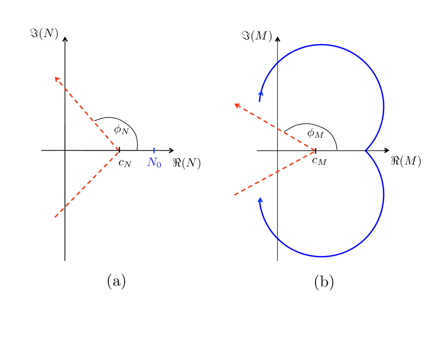
Figure 1: Contours for the inverse Mellin transforms, (a) for ${\cal C}_{N}$, (b) for ${\cal C}_{M}$. We have defined $N_{0}=L_{0}/c_{M}$, with $L_{0}$ given in (32). In (b), the solid line depicts the location of the Landau pole as $N$ moves along a part of its contour (see text).

As the exponentiation of soft-gluon corrections is achieved in Mellin moment space, the hadronic structure function is obtained by taking the inverse Mellin transforms of Eq. (8):

$${\cal F}^{h}_{i}(x,z,Q^{2})=\int_{{\cal C}_{N}}\frac{dN}{2\pi i}x^{-N}\int_{{\cal C}_{M}}\frac{dM}{2\pi i}z^{-M}\tilde{{\cal F}}^{h}_{i}(N,M,Q^{2}),$$ (31)

where ${\cal C}_{N}$ and ${\cal C}_{M}$ denote integration contours in the complex plane, one for each Mellin inverse. When performing an inverse Mellin transform, the contour usually has to be chosen in such a way that all singularities of the integrand lie to its left. However, as can be seen from Eq. (II.3),(II.3), the resummed cross section has a Landau singularity at $\lambda_{NM}=1$ or

$$N\,M={\mathrm{e}}^{1/(\alpha_{s}b_{0})-2\gamma_{E}}\equiv L_{0},$$ (32)

as a result of the divergence of the running coupling $\alpha_{s}$ in Eq. (20) for $k_{\perp}\to\Lambda_{\mathrm{QCD}}$. For the Mellin inversions, we adopt the minimal prescription developed in Ref. Catani:1996yz to deal with the Landau pole. For this prescription the contours are chosen to lie to the left of the Landau singularity. In order to achieve this, we first choose the contour for the $N$-integration in the upper complex half plane in the standard way (see Fig. 1(a)) as

$$N=c_{N}+z_{N}\,{\mathrm{e}}^{i\phi_{N}},$$ (33)

where $c_{N}$ is a postive real constant, $\phi_{N}\sim 3\pi/4$ and $z_{N}\in[0,\infty]$. For the lower branch of the contour, one simply uses the complex conjugate of $N$. The contour for the $M$-integration is parameterized in a similar fashion, with a constant $c_{M}$, an integration parameter $z_{M}$ and an angle $\phi_{M}$ that we will address shortly. The fact that both contours are tilted into the half-plane with negative real part improves the numerical convergence of the integration, since contributions with negative real part are exponentially suppressed by the factors $x^{-N}$, $z^{-M}$ in Eq. (31).

In accordance with the minimal prescription Catani:1996yz , the parameter $c_{N}$ is chosen to be smaller than $N_{0}\equiv L_{0}/c_{M}$. As $N$ moves along its contour from a point with large negative imaginary part to a point with large positive one, the Landau pole given by Eq. (32) describes a trajectory shown by the solid line in Fig. 1(b). The angle $\phi_{M}$ is now chosen in such a way that the $M$-integration contour (shown by the dashed line) avoids this trajectory. The larger the imaginary part of $N$, the larger the angle $\phi_{M}$ needs to become. Of course, ultimately as $\Im(N)\to\pm\infty$, the Landau pole moves to the origin in the $M$-plane, and the contour falls onto the real $M$-axis. However, as described above, the contributions from such large values of $N$ are extremely suppressed. We note that a similar approach to the choice of contours was discussed in Ref. Sterman:2000pt , where combined inverse Mellin and Fourier transforms were considered. An alternative approach is to expand the resummed formula to high perturbative orders. At each finite order, the Landau pole is not present and, therefore, standard Mellin contours can be chosen.

We match the resummed cross section to the NLO one by subtracting the $O(\alpha_{s})$ expansion of the resummed expression and adding the full NLO cross section. This “matched” cross section consequently not only resums the large threshold logarithms to all orders, but also contains the full NLO results for the $q\to q$, $q\to g$ and $g\to q$ channels. We will occasionally also consider a resummed cross section that has not been matched to the NLO one. We will refer to such a cross section as “unmatched”.

II.5 Resummation for inclusive DIS

In order to obtain resummed predictions for the SIDIS hadron multiplicities defined in (3), we also need the resummation for the inclusive cross section. In this case, there is only one variable $x$, and standard Mellin-moment resummation techniques Schaefer:2001uh ; neubert may be applied. The inclusive structure functions ${\cal F}_{T}$ and ${\cal F}_{L}$ introduced in Eq. (4) can be written as

$${\cal F}_{i}(x,Q^{2})=\sum_{f}\int_{x}^{1}\frac{d\hat{x}}{\hat{x}}f\left(\frac{x}{\hat{x}},\mu^{2}\right){\cal{C}}^{i}_{f}\left(\hat{x},\frac{Q^{2}}{\mu^{2}},\alpha_{s}(\mu^{2})\right).$$ (34)

We refer the reader to Ref. fupe for the NLO expressions for the coefficient functions ${\cal{C}}^{i}_{f}$. Resummation may be performed by again introducing Mellin moments in $x$. The resummed DIS coefficient function for the structure function ${\cal F}_{T}$ reads to NLL in moment space:

$$\tilde{\cal{C}}^{T,{\mathrm{res}}}_{q} = e_{q}^{2}H_{q}\left(\alpha_{s}(Q^{2}),\frac{Q^{2}}{\mu^{2}}\right)\exp\left[\int_{0}^{1}d\xi\frac{\xi^{N}-1}{1-\xi}\right.$$

$$\left.\times\left\{\int_{Q^{2}}^{(1-\xi)Q^{2}}\frac{dk_{\perp}^{2}}{k_{\perp}^{2}}A_{q}(\alpha_{s}(k_{\perp}^{2}))+\frac{1}{2}B_{q}\left(\alpha_{s}((1-\xi)Q^{2})\right)\right\}\right],$$

where the function $A_{q}(\alpha_{s})$ is as in (16). The perturbative function $B_{q}(\alpha_{s})$ is given by

$$B_{q}(\alpha_{s})=\frac{\alpha_{s}}{\pi}B_{q}^{(1)}+{\cal O}(\alpha_{s}^{2}),$$ (36)

with

$$B_{q}^{(1)}=-\frac{3}{2}C_{F}.$$ (37)

Finally, the hard-scattering coefficient reads

$$H_{q}\left(\alpha_{s}(Q^{2}),\frac{Q^{2}}{\mu^{2}}\right)=1+\frac{\alpha_{s}}{2\pi}C_{F}\left(-\frac{9}{2}-\frac{\pi^{2}}{6}+\frac{3}{2}\ln\frac{Q^{2}}{\mu^{2}}\right)$$

$$\hskip 93.89418pt+{\cal O}(\alpha_{s}^{2}).$$ (38)

The exponential in (II.5) can evidently be written as $\Delta_{q}^{N}\times J_{q}^{N}$, where

$$\log\Delta_{q}^{N} \equiv \left[\int_{0}^{1}dx\frac{\xi^{N}-1}{1-\xi}\int_{Q^{2}}^{(1-\xi)^{2}Q^{2}}\frac{dk_{\perp}^{2}}{k_{\perp}^{2}}A_{q}(\alpha_{s}(k_{\perp}^{2}))\right],$$

$$\log J_{q}^{N} \equiv \left[\int_{0}^{1}d\xi\frac{\xi^{N}-1}{1-\xi}\left\{\int_{(1-\xi)^{2}Q^{2}}^{(1-\xi)Q^{2}}\frac{dk_{\perp}^{2}}{k_{\perp}^{2}}A_{q}(\alpha_{s}(k_{\perp}^{2}))\right.\right.$$ (39)

$$\hskip 11.38109pt\left.+\frac{1}{2}B_{q}(\alpha_{s}((1-\xi)Q^{2}))\right\}\Bigg{]}.$$

The NLL expansions of these functions can be performed in the same way as described in the previous subsection. One obtains:

$$\log\Delta_{q}^{N}\,=\,\ln\bar{N}h_{q}^{(1)}(\lambda)+h_{q}^{(2)}\left(\lambda,\frac{Q^{2}}{\mu^{2}},\frac{Q^{2}}{\mu_{F}^{2}}\right),$$ (40)

with the functions $h_{q}^{(1)},h_{q}^{(2)}$ given in (II.3). Furthermore,

$$\ln J_{q}^{N}=\ln\bar{N}f_{q}^{(1)}(\lambda)+f_{q}^{(2)}\left(\lambda,\frac{Q^{2}}{\mu^{2}}\right),$$ (41)

with Schaefer:2001uh

$$f_{q}^{(1)}(\lambda) = h_{q}^{(1)}\left(\frac{\lambda}{2}\right)-h_{q}^{(1)}(\lambda),$$

$$f_{q}^{(2)}\left(\lambda,\frac{Q^{2}}{\mu^{2}}\right) = 2h_{q}^{(2)}\left(\frac{\lambda}{2},\frac{Q^{2}}{\mu^{2}},1\right)-h_{q}^{(2)}\left(\lambda,\frac{Q^{2}}{\mu^{2}},1\right)$$ (42)

$$+ \frac{B_{q}^{(1)}}{2\pi b_{0}}\ln(1-\lambda).$$

III Resummation for $e^{+}e^{-}\to hX$

Hadron multiplicities in $e^{+}e^{-}\to hX$ are defined by

$$R^{h}_{e^{+}e^{-}}\equiv\frac{1}{\sigma^{\mathrm{tot}}}\frac{d^{2}\sigma^{h}}{dx_{E}d\cos\theta},$$ (43)

where $d^{2}\sigma^{h}/dx_{E}d\cos\theta$ is the differential cross section for the production of the hadron $h$ at angle $\theta$ relative to the initial positron. Furthermore,

$$x_{E}\equiv\frac{2P_{h}\cdot q}{Q^{2}},$$ (44)

where $P_{h}$ and $q$ are the momenta of the produced hadron and the intermediate virtual photon respectively and $Q^{2}=q^{2}$. $\sigma^{\mathrm{tot}}$ is the total cross section for $e^{+}e^{-}\to{\mathrm{hadrons}}$. To first order in $\alpha_{s}$ it reads:

$$\sigma^{\mathrm{tot}}=\frac{4\pi\alpha^{2}}{3Q^{2}}N_{C}\sum_{q}e_{q}^{2}\left(1+\frac{\alpha_{s}}{\pi}\right),$$ (45)

where $N_{C}=3$ is the number of colors.

As in the case of SIDIS, one can write the cross section $d^{2}\sigma^{h}/dx_{E}d\cos\theta$ in terms of structure functions fupe ; Nason:1993xx :

$$\frac{d^{2}\sigma^{h}}{dx_{E}d\cos\theta} = \frac{\pi\alpha^{2}}{Q^{2}}N_{C}\left[\frac{1+\cos^{2}\theta}{2}\hat{{\cal F}}^{h}_{T}(x_{E},Q^{2})\right.$$ (46)

$$+\sin^{2}\theta\,\hat{{\cal F}}^{h}_{L}(x_{E},Q^{2})\Big{]},$$

where

$$\hat{{\cal F}}_{i}^{h}(x_{E},Q^{2})=\sum_{f}\int_{x_{E}}^{1}\frac{d\hat{z}}{\hat{z}}D_{f}^{h}\left(\frac{x_{E}}{\hat{z}},\mu^{2}\right)\hat{{\cal{C}}}^{i}_{f}\left(\hat{z},\frac{Q^{2}}{\mu^{2}},\alpha_{s}(\mu^{2})\right),$$ (47)

with the fragmentation functions $D_{f}^{h}$ introduced in subsection II.1. To lowest order, only the partonic channel $e^{+}e^{-}\to qX$ contributes, for which

$$\hat{C}^{T,(0)}_{q}(\hat{z}) = e_{q}^{2}\,\delta(1-\hat{z}),$$

$$\hat{C}^{L,(0)}_{q}(\hat{z}) = 0.$$ (48)

Again we refer the reader to the previous literature altarelli ; fupe ; Kretzer:2000yf for the NLO expressions for the coefficient functions. After taking Mellin moments in $x_{E}$, the resummed result for the corresponding hard-scattering function turns out to be identical to that in (II.5) Cacciari:2001cw ; Blum ; Vogt , except for a change $-\pi^{2}/6\to 5\pi^{2}/6$ in the coefficient $H_{q}$ in (II.5).

IV Phenomenological Results

We now investigate the numerical size of the threshold resummation effects for the two semi-inclusive hadron production processes discussed above, SIDIS and $e^{+}e^{-}\to hX$. We focus entirely on pion production in this work, for which the theory is expected to be under best control. We also consider a proton target throughout this work. For the parton distribution functions we use the NLO “Martin–Stirling–Thorne–Watt” (MSTW 2008) set of Martin:2009iq , whereas we choose the NLO “de Florian–Sassot–Stratmann” (DSS) defloriandss pion fragmentation functions. In this set, fragmentation functions for charged pions $\pi^{\pm}$ are separately available. We note that the parton distributions and fragmentation functions are provided in $x$ (or $z$) space, whereas according to Eq. (9) we need their Mellin moments. To obtain the latter, we first fit suitable functions of the form $Ax^{\alpha}(1-x)^{\beta}$ times a polynomial in $x$ to the distributions. It is then straightforward to take Mellin moments of the fitted functions analytically and use them in the numerical code. We have checked that the accuracy of the fit is overall very good.

IV.1 Results for SIDIS

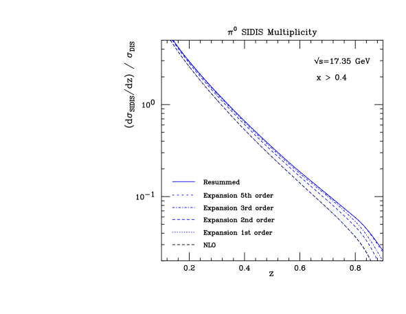
Figure 2: SIDIS multiplicity for $\pi^{0}$. Kinematics are as for the COMPASS measurements compass (see text) with, however, an additional cut $x>0.4$ to enhance the contribution from the threshold regime. The lower two lines which are almost indistinguishable show the NLO result and the first-order expansion of the resummed result (without matching). The top line shows the full NLL resummed result; the lines in between display various fixed-order expansions of the latter.

We start by examining the overall effects of threshold resummation for SIDIS, using the kinematics relevant for the COMPASS SIDIS measurements compass as an example. COMPASS uses a muon beam of energy 160 GeV incident on a proton fixed target. The resulting center-of-mass energy is $\sqrt{s}\approx$17.4 GeV. The kinematic cuts employed by COMPASS are $0.041<x<0.7$, $0.1<y<0.9$, $Q^{2}>1$ GeV² and $W^{2}=Q^{2}(1-x)/x+m_{p}^{2}>49$ GeV², where $m_{p}$ is the proton mass. We choose the renormalization and factorization scales as $Q$ and consider the SIDIS multiplicity for neutral pions $\pi^{0}$ as a function of $z$, but integrating numerator and denominator of Eq. (3) over $x$ and $y$. We observe that the range of $x$ probed by the full COMPASS data sample extends down to fairly low values, where one could be quite far from the threshold regime. We therefore first consider a lower cut of $x>0.4$. Figure 2 shows our results for the NLO and the resummed multiplicities, along with those for expansions of the resummed cross section to various finite orders in $\alpha_{s}$. In each case, the denominator of the multiplicity, the inclusive-DIS cross section, has been treated in the same fashion as the SIDIS one in the numerator. With the exception of the first-order expansion, all beyond-NLO results have been matched to the NLO one (separately in the numerator and the denominator) as described at the end of Sec.II.4. We first of all note that the first-order expansion of the resummed cross section agrees very well with the full NLO one, which demonstrates that for the chosen kinematics the threshold regime strongly dominates the NLO cross section. The full resummed result shows a marked increase over the NLO one, in particular at high $z$, and the higher-order expansions converge nicely to the resummed result. Clearly, the $\alpha_{s}^{2}$ and $\alpha_{s}^{3}$ contributions generated by resummation are still significant.

The results can also be studied as ratios $({\mathrm{Th^{\prime}-NLO}})/{\mathrm{NLO}}$, where ${\mathrm{Th^{\prime}}}$ denotes any of the higher-order SIDIS multiplicities generated by resummation. Figure 3 shows these ratios for the unmatched first-order expansion, the matched higher-order expansions and the full resummed result. The good agreement of NLO and the first-order expansion is evident, as are the large resummation effects at high $z$.

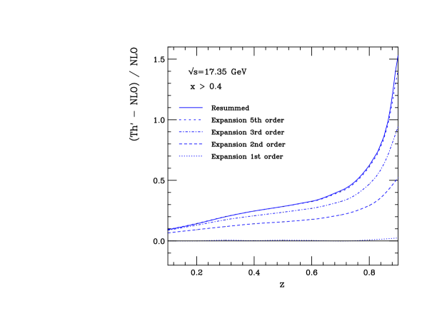
Figure 3: Ratios $({\mathrm{Th^{\prime}-NLO}})/{\mathrm{NLO}}$, where ${\mathrm{Th^{\prime}}}$ corresponds to the SIDIS multiplicity at higher orders as generated by resummation. The first-order expansion of the resummed cross section has not been matched since it would otherwise be identical to NLO.

We now extend the $x$-range to the full region $0.041<x<0.7$ covered by COMPASS. Figs. 4 and 5 show the corresponding results, where all lines directly correspond to the ones shown in Figs. 2 and 3 for the case $x>0.4$. One can see that the resummation effects are generally smaller now, even though they remain significant at high $z$. As expected, the agreement between NLO and the first-order expansion of the resummed cross section is worse now, but it typically remains at the 10% level or better. The second-order expansion captures most of the full resummation effects; the yet higher orders converge somewhat more slowly now to the resummed result. Figure 5 shows the corresponding ratios $({\mathrm{Th^{\prime}-NLO}})/{\mathrm{NLO}}$, where again ${\mathrm{Th^{\prime}}}$ denotes any of the SIDIS multiplicities computed at higher orders.

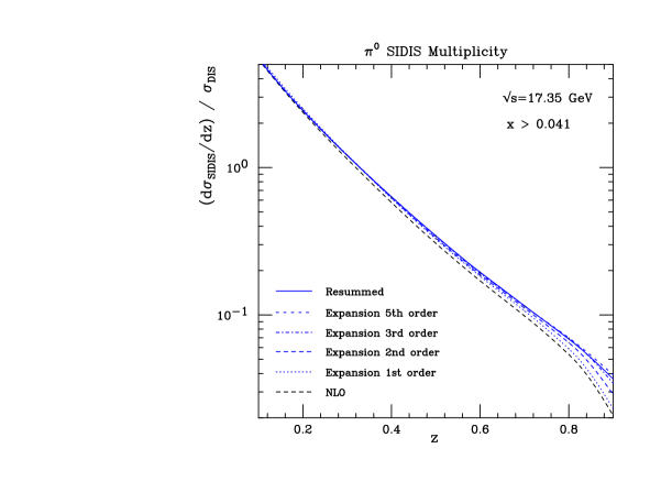
Figure 4: Same as Fig. 2, but for $x>0.041$.

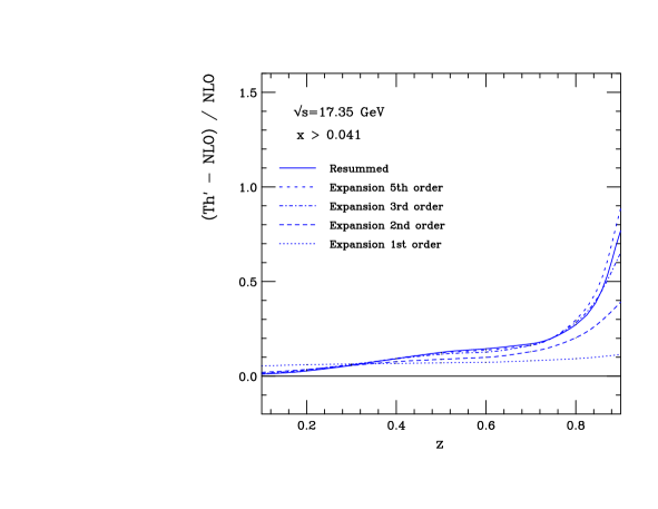
Figure 5: Same as Fig. 3, but for $x>0.041$.

Preliminary precise data from COMPASS for charged-pion and kaon multiplicities are available for a wide range of kinematics compass . The full data set, which evidently has the best statistics, covers the range used above for Figs. 4 and 5. Figures 6 and 7 show comparisons of our NLO and NLL resummed calculations for charged pions to the COMPASS data. As one can see, resummation leads to a moderate, but significant, enhancement of the multiplicities. It is interesting to note that such an enhancement is in fact preferred by the $\pi^{-}$ data. However, we do not assign much importance to this observation. The fragmentation functions are presently still not very well determined and a different set (or a new fit) might well describe the data also at NLO. Our main point is that inclusion of resummation effects in an analysis of fragmentation functions could make a significant difference for the extracted functions.

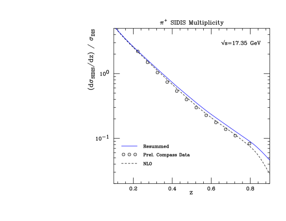
Figure 6: NLO and NLL resummed SIDIS multiplicities for $\pi^{+}$. The results are compared to the preliminary COMPASS data compass . The uncertainties of the data are smaller than the symbol size used in the plot.

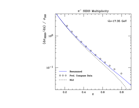
Figure 7: Same as Fig. 6, but for $\pi^{-}$.

Figures 8 and 9 show similar comparisons to the HERMES preliminary data hermes . For this data set, the center-of-mass energy is $\sqrt{s}\approx$17.4 GeV. The kinematic cuts employed by HERMES are $0.023<x<0.6$, $0.1<y<0.85$, $Q^{2}>1$ GeV² and $W^{2}=10$ GeV². The results are qualitatively similar to those shown for COMPASS kinematics.

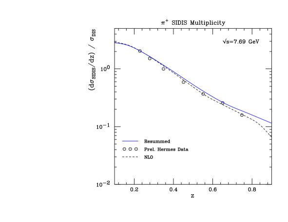
Figure 8: Same as Fig. 6, but for HERMES kinematics. The preliminary data are from hermes . The uncertainties of the data are smaller than the symbol size used in the plot.

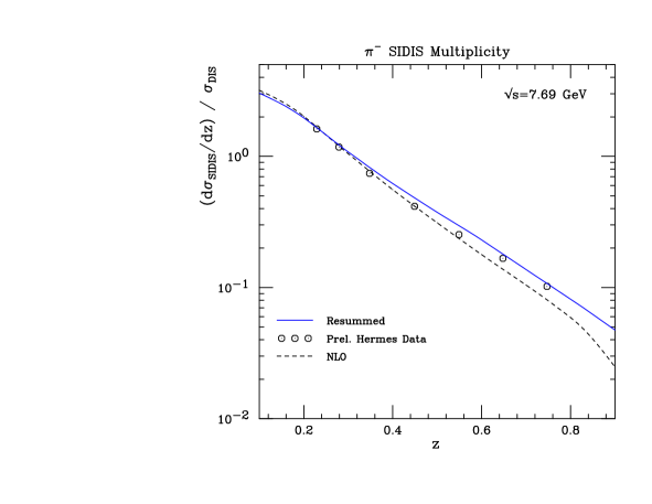
Figure 9: Same as Fig. 8, but for $\pi^{-}$.

IV.2 Results for single-inclusive $e^{+}e^{-}$ annihilation

Figure 10 presents our results for the $\pi^{-}$ multiplicity in $e^{+}e^{-}$ annihilation at $\sqrt{s}=10.52$ GeV and for $-1<\cos\theta<1$, as appropriate for comparison to the forthcoming BELLE data belle . The $\pi^{+}$ multiplicity is identical thanks to charge conjugation symmetry. We have chosen the factorization and renormalization scales as $\sqrt{s}$. As for SIDIS, we show NLO and NLL resummed results, along with various fixed-order expansions of the resummed multiplicity. One first of all observes the excellent agreement between the NLO result and the first-order expansion of the resummed one. This clearly demonstrates that the threshold regime strongly dominates for the BELLE kinematics. We can therefore be confident that also the resummed result reliably captures the important higher-order terms. Resummation leads to a significant enhancement of the $\pi^{-}$ multiplicity. This enhancement becomes particularly strong at high $x_{E}$, but is present also at moderate values. Figure 11 shows the corresponding ratios $({\mathrm{Th^{\prime}-NLO}})/{\mathrm{NLO}}$, where ${\mathrm{Th^{\prime}}}$ denotes any of the higher-order multiplicities generated by resummation and shown in Fig. 10. Since the precision of the preliminary BELLE data is typically much better than 10%, it will be important to include the enhancements we find in future global analyses of fragmentation functions, similar to what has been done in the past in Ref. akk .

Figure 10: $\pi^{-}$ multiplicity in electron-positron annihilation at $\sqrt{s}=10.52$ GeV. The two lowest lines show the NLO result and the (unmatched) first-order expansion of the resummed one, which are practically indistinguishable. The other lines show matched higher-order expansions of the resummed multiplicity, and the resummed result itself (solid line).

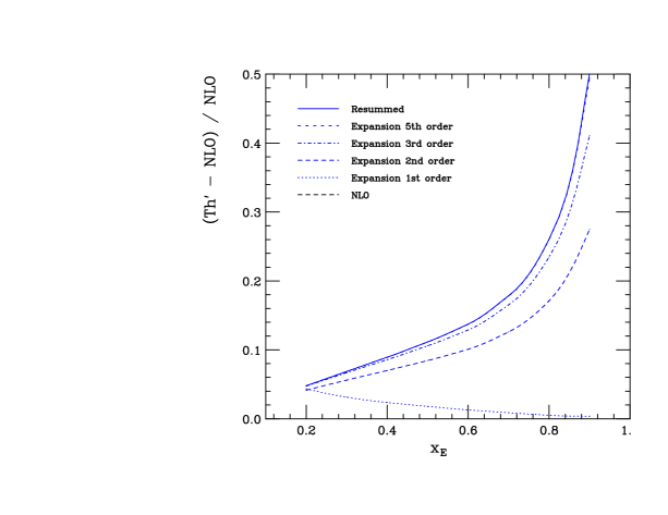
Figure 11: Ratios $({\mathrm{Th^{\prime}-NLO}})/{\mathrm{NLO}}$ corresponding to the various curves shown in Fig. 10.

V Conclusions

We have derived threshold-resummed expressions for the coefficient functions for single-inclusive hadron production in semi-inclusive lepton scattering and $e^{+}e^{-}$ annihilation. We have presented phenomenological results for pion multiplicities for these processes in the kinematic regimes presently accessed by the COMPASS, HERMES and BELLE experiments. We have found that resummation leads to modest but significant enhancements of the multiplicities. The recent preliminary SIDIS data turn out to be overall better described when resummation effects are included in the calculation, at least for the DSS set of fragmentation functions that we have used. However, we do not ascribe much significance to this point as the fragmentation functions are still rather poorly constrained so that a new NLO fit to the new data would likely also work well strat . Our main point is that, given the good accuracy of the new preliminary SIDIS and BELLE data, it will be crucial to include resummation effects for both processes in the next generation of analyses of fragmentation functions. In fact, because of the enhancements from threshold resummation, the extracted fragmentation functions would be expected to be softer or smaller at high $z$ than functions extracted purely on the basis of an NLO framework. This may well have important ramifications for the QCD predictions obtained for other processes sensitive to fragmentation functions. For instance, it has recently been observed strat ; dent that the ALICE data Abelev:2012cn for neutral-pion production at 7 TeV are well below the theoretical NLO expectations. One may speculate if this is due in part to fragmentation functions that are too large at high $z$.

We note that at very high $z$ or $x_{E}$, besides the logarithmic perturbative corrections also nonperturbative power corrections will ultimately become relevant and will need to be analyzed theoretically. Resummation offers ways to address these contributions (see, for example Sterman:2006hu ; power , and references therein). Based on the ideas presented there, we do not think that power corrections play an overwhelming role in the presently accessible kinematic regime in SIDIS. As we saw in Eq. (II.3), the logarithmic contributions to SIDIS come from the region $k_{\perp}\gtrsim Q/\sqrt{\bar{N}\bar{M}}$. In $x$-$z$-space this scale roughly corresponds to $Q\sqrt{(1-z)(1-x)}$. We have checked that for COMPASS kinematics even at $z=0.9$ the average value of this scale is significantly larger than 1 GeV, implying that perturbation theory should still provide a reliable answer here. This issue obviously deserves a more detailed investigation in the future, in particular also for the case of $e^{+}e^{-}$ annihilation.

We stress that our study may be extended in several ways. First, as mentioned in the Introduction, resummation for $e^{+}e^{-}\to hX$ could be carried out at next-to-next-to-leading logarithm and even beyond, thanks to Blum ; Vogt . The high precision of the BELLE data may well warrant a future study along these lines. Resummation for SIDIS could probably also be extended to next-to-next-to-leading logarithmic accuracy with some moderate further developments. This may become a very worthwhile task in the future when high-precision SIDIS data will become available from measurements at the Jefferson Laboratory after the CEBAF upgrade to 12 GeV beam energy Burkert:2012rh . Finally, one may readily adapt the resummation framework to the case of polarized SIDIS, which serves as an important probe of the spin structure of the nucleon. Present polarized-SIDIS measurements have the same kinematics as those considered in this paper.

VI Acknowledgments

We thank M. Traini for helpful discussions and M. Leitgab for useful communications on the BELLE measurements.

Appendix

In this Appendix we collect the NLO expressions for the spin-averaged partonic SIDIS cross sections. At NLO, we have to consider the processes $\gamma^{*}q\to qX$, $\gamma^{*}q\to gX$, and $\gamma^{*}g\to qX$. For their contributions to the structure function ${\cal F}_{T}^{h}$ we have in the $\overline{\mathrm{MS}}$ scheme altarelli ; Nason:1993xx ; fupe ; graudenz ; deFlorian:1997zj ; roth :

$$C_{qq}^{T,(1)}(\hat{x},\hat{z}) = e_{q}^{2}C_{F}\Bigg{[}-8\delta(1-\hat{x})\delta(1-\hat{z})$$ (49)

$$+\delta(1-\hat{x})\left[\tilde{P}_{qq}(\hat{z})\ln\frac{Q^{2}}{\mu_{F}^{2}}+L_{1}(\hat{z})+L_{2}(\hat{z})+(1-\hat{z})\right]$$

$$+\delta(1-\hat{z})\left[\tilde{P}_{qq}(\hat{x})\ln\frac{Q^{2}}{\mu_{F}^{2}}+L_{1}(\hat{x})-L_{2}(\hat{x})+(1-\hat{x})\right]$$

$$+\frac{2}{(1-\hat{x})_{+}(1-\hat{z})_{+}}-\frac{1+\hat{z}}{(1-\hat{x})_{+}}-\frac{1+\hat{x}}{(1-\hat{z})_{+}}$$

$$+2(1+\hat{x}\hat{z})\Bigg{]},$$

$$C_{gq}^{T,(1)}(\hat{x},\hat{z}) = e_{q}^{2}C_{F}\Bigg{[}\tilde{P}_{gq}(\hat{z})\left(\delta(1-\hat{x})\ln\left(\frac{Q^{2}}{\mu_{F}^{2}}\hat{z}(1-\hat{z})\right)\right.$$

$$\left.+\frac{1}{(1-\hat{x})_{+}}\right)+\hat{z}\delta(1-\hat{x})+2(1+\hat{x}-\hat{x}\hat{z})-\frac{1+\hat{x}}{\hat{z}}\Bigg{]},$$

$$C_{qg}^{T,(1)}(\hat{x},\hat{z}) = e_{q}^{2}T_{R}\Bigg{[}\delta(1-\hat{z})\left[\tilde{P}_{qg}(\hat{x})\ln\left(\frac{Q^{2}}{\mu_{F}^{2}}\frac{1-\hat{x}}{\hat{x}}\right)\right.$$ (51)

$$+2\hat{x}(1-\hat{x})\Big{]}+\tilde{P}_{qg}(\hat{x})\left\{\frac{1}{(1-\hat{z})_{+}}+\frac{1}{\hat{z}}-2\right\}\Bigg{]},$$

where $e_{q}$ is the quark’s fractional charge, $C_{F}=4/3$, $T_{R}=1/2$,

$$\tilde{P}_{qq}(\xi)=\frac{1+\xi^{2}}{(1-\xi)_{+}}+\frac{3}{2}\delta(1-\xi),$$

$$\tilde{P}_{gq}(\xi)=\frac{1+(1-\xi)^{2}}{\xi},$$

$$\tilde{P}_{qg}(\xi)=\xi^{2}+(1-\xi)^{2},$$

$$L_{1}(\xi)=(1+\xi^{2})\left(\frac{\ln(1-\xi)}{1-\xi}\right)_{+},$$

$$L_{2}(\xi)=\frac{1+\xi^{2}}{1-\xi}\ln\xi,$$ (52)

and the “+” - distributions are defined as follows:

$$\int_{0}^{1}d\xi f(\xi)[g(\xi)]_{+} \equiv \int_{0}^{1}d\xi\left(f(\xi)-f(1)\right)g(\xi),$$

$$\int_{0}^{1}d\hat{x}\int_{0}^{1}d\hat{z}\frac{f(\hat{x},\hat{z})}{(1-\hat{x})_{+}(1-\hat{z})_{+}}$$

$$\equiv\int_{0}^{1}d\hat{x}\int_{0}^{1}d\hat{z}\,\frac{f(\hat{x},\hat{z})-f(1,\hat{z})-f(\hat{x},1)+f(1,1)}{(1-\hat{x})(1-\hat{z})}.$$

Note that we have given expressions (49)-(51) for an arbitrary factorization scale $\mu_{F}$, keeping however the scales the same for the initial and the final state. For the longitudinal structure function $F^{h}_{L}$:

$$C_{qq}^{L,(1)}(\hat{x},\hat{z}) = 4e_{q}^{2}C_{F}\hat{x}\hat{z},$$

$$C_{gq}^{L,(1)}(\hat{x},\hat{z}) = 4e_{q}^{2}C_{F}\hat{x}(1-\hat{z}),$$

$$C_{qg}^{L,(1)}(\hat{x},\hat{z}) = 8e_{q}^{2}T_{R}\hat{x}(1-\hat{x}).$$ (54)

In Mellin-moment space, the NLO results become Stratmann:2001pb

$$\tilde{C}_{qq}^{T,(1)}(N,M) = e_{q}^{2}C_{F}\Bigg{[}-8-\frac{1}{M^{2}}+\frac{2}{(M+1)^{2}}+\frac{1}{N^{2}}$$ (55)

$$+\frac{(1+M+N)^{2}+1}{M(M+1)N(N+1)}+3S_{2}(M)-S_{2}(N)$$

$$+\left[S_{1}(M)+S_{1}(N)\right]\Bigg{\{}S_{1}(M)+S_{1}(N)$$

$$\left.-\frac{1}{M(M+1)}-\frac{1}{N(N+1)}\right\}$$

$$+\left[\frac{1}{N(N+1)}+\frac{3}{2}-2S_{1}(N)\right]\ln\left(\frac{Q^{2}}{\mu_{F}^{2}}\right)$$

$$+\left[\frac{1}{M(M+1)}+\frac{3}{2}-2S_{1}(M)\right]\ln\left(\frac{Q^{2}}{\mu_{F}^{2}}\right)\Bigg{]},$$

$$\tilde{C}_{gq}^{T,(1)}(N,M) = e_{q}^{2}C_{F}\Bigg{[}\frac{2-2M-9M^{2}+M^{3}-M^{4}+M^{5}}{M^{2}(M-1)^{2}(M+1)^{2}}$$ (56)

$$+\frac{2M}{N(M+1)(M-1)}-\frac{2-M+M^{2}}{M(M+1)(M-1)(N+1)}$$

$$-\frac{2+M+M^{2}}{M(M+1)(M-1)}\left[S_{1}(M)+S_{1}(N)\right]$$

$$+\frac{2+M+M^{2}}{M(M+1)(M-1)}\ln\left(\frac{Q^{2}}{\mu_{F}^{2}}\right)\Bigg{]},$$

$$\tilde{C}_{qg}^{T,(1)}(N,M) = e_{q}^{2}T_{R}\Bigg{[}\frac{2+N+N^{2}}{N(N+1)(N+2)}\Bigg{(}\frac{1}{M-1}-\frac{1}{M}$$ (57)

$$-S_{1}(M)-S_{1}(N)+\ln\left(\frac{Q^{2}}{\mu_{F}^{2}}\right)\Bigg{)}+\frac{1}{N^{2}}\Bigg{]},$$

where

$$S_{i}(N)\equiv\sum_{j=1}^{N}\frac{1}{j^{i}}\;.$$ (58)

Note that at large $N$ we have

$$S_{1}(N)=\ln\bar{N}+{\cal O}(1/N),\;\;S_{2}(N)=\frac{\pi^{2}}{6}+{\cal O}(1/N),$$ (59)

where $\bar{N}=N{\mathrm{e}}^{\gamma_{E}}$. Furthermore, for the longitudinal structure function,

$$\tilde{C}_{qq}^{L,(1)}(N,M) = e_{q}^{2}C_{F}\frac{4}{(M+1)(N+1)},$$ (60)

$$\tilde{C}_{gq}^{L,(1)}(N,M) = e_{q}^{2}C_{F}\frac{4}{M(M+1)(N+1)},$$ (61)

$$\tilde{C}_{qg}^{L,(1)}(N,M) = e_{q}^{2}T_{R}\frac{8}{M(N+1)(N+2)}.$$ (62)

Here we have corrected a mistake in $\tilde{C}_{qg}^{L,(1)}(N,M)$ in Ref. Stratmann:2001pb .

References

- (1) D. de Florian, R. Sassot and M. Stratmann, Phys. Rev. D 75, 114010 (2007) [hep-ph/0703242]; M. Epele, R. Llubaroff, R. Sassot and M. Stratmann, Phys. Rev. D 86, 074028 (2012) [arXiv:1209.3240 [hep-ph]].
- (2) M. Stratmann, talk presented at the “Workshop on Fragmentation Functions and QCD 2012 (Fragmentation 2012)”, RIKEN, Japan, November 2012.
- (3) S. Albino, B. A. Kniehl and G. Kramer, Nucl. Phys. B 803, 42 (2008) [arXiv:0803.2768 [hep-ph]].
- (4) M. Hirai, S. Kumano, T. -H. Nagai and K. Sudoh, Phys. Rev. D 75, 094009 (2007) [hep-ph/0702250].
- (5) For review, see, for example: M. Burkardt, C. A. Miller and W. D. Nowak, Rept. Prog. Phys. 73, 016201 (2010) [arXiv:0812.2208 [hep-ph]].
- (6) M. Leitgab [Belle Collaboration], arXiv:1210.2137 [nucl-ex].
- (7) S. Joosten [Hermes Collaboration], talk presented at the “XIX International Workshop on Deep-Inelastic Scattering and Related Subjects (DIS 2011)”, April 2011, Newport News, VA USA.
- (8) N. Makke [Compass Collaboration], PhD thesis Measurement of the polarization of strange quarks in the nucleon and determination of quark fragmentation functions into hadrons, CERN-THESIS-2011-279.
- (9) G. F. Sterman and W. Vogelsang, Phys. Rev. D 74, 114002 (2006) [hep-ph/0606211].
- (10) G. F. Sterman, AIP Conf. Proc. 74, 22 (1981); J. G. M. Gatheral, Phys. Lett. B 133, 90 (1983); J. Frenkel and J. C. Taylor, Nucl. Phys. B 246, 231 (1984); C. F. Berger, hep-ph/0305076.
- (11) E. Laenen, G. F. Sterman and W. Vogelsang, Phys. Rev. D 63, 114018 (2001) [hep-ph/0010080]; Phys. Rev. Lett. 84, 4296 (2000) [hep-ph/0002078].
- (12) M. Cacciari and S. Catani, Nucl. Phys. B 617, 253 (2001) [hep-ph/0107138].
- (13) J. Blumlein and V. Ravindran, Phys. Lett. B 640, 40 (2006) [hep-ph/0605011].
- (14) S. Moch and A. Vogt, Phys. Lett. B 680, 239 (2009) [arXiv:0908.2746 [hep-ph]].
- (15) See also: M. Procura and W. J. Waalewijn, Phys. Rev. D 85, 114041 (2012) [arXiv:1111.6605 [hep-ph]].
- (16) S. Catani and L. Trentadue, Nucl. Phys. B 327, 323 (1989).
- (17) G. Bozzi, S. Catani, D. de Florian and M. Grazzini, Nucl. Phys. B 791, 1 (2008) [arXiv:0705.3887 [hep-ph]].
- (18) W. Vogelsang, AIP Conf. Proc. 747, 9 (2005).
- (19) G. Altarelli, R.K. Ellis, G. Martinelli, and S.Y. Pi, Nucl. Phys. B160, 301 (1979).
- (20) P. Nason and B. R. Webber, Nucl. Phys. B 421, 473 (1994) [Erratum-ibid. B 480, 755 (1996)].
- (21) W. Furmanski and R. Petronzio, Z. Phys. C11, 293 (1982).
- (22) D. Graudenz, Nucl. Phys. B432, 351 (1994).
- (23) D. de Florian, M. Stratmann and W. Vogelsang, Phys. Rev. D 57, 5811 (1998) [hep-ph/9711387].
- (24) D. de Florian and Y. R. Habarnau, arXiv:1210.7203 [hep-ph].
- (25) M. Stratmann and W. Vogelsang, Phys. Rev. D 64, 114007 (2001) [hep-ph/0107064].
- (26) S. Catani, M. L. Mangano, P. Nason and L. Trentadue, Nucl. Phys. B 478, 273 (1996) [arXiv:hep-ph/9604351].
- (27) G. F. Sterman and W. Vogelsang, JHEP 0102, 016 (2001) [hep-ph/0011289].
- (28) A. Vogt, Phys. Lett. B 497, 228 (2001) [hep-ph/0010146]; S. Schaefer, A. Schäfer and M. Stratmann, Phys. Lett. B 514, 284 (2001) [hep-ph/0105174]; see also: E. Gardi and R. G. Roberts, Nucl. Phys. B 653, 227 (2003) [hep-ph/0210429]; G. Corcella and L. Magnea, Phys. Rev. D 72, 074017 (2005) [hep-ph/0506278]; M. Osipenko et al., Phys. Rev. D 71, 054007 (2005) [hep-ph/0503018]; G. Grunberg, Phys. Lett. B 687, 405 (2010) [arXiv:0911.4471 [hep-ph]].
- (29) For an alternative approach that does not resort to Mellin moments, see: T. Becher, M. Neubert and B. D. Pecjak, JHEP 0701, 076 (2007) [hep-ph/0607228].
- (30) S. Kretzer, Phys. Rev. D 62, 054001 (2000) [hep-ph/0003177].
- (31) A. D. Martin, W. Stirling, R. Throne and G. Watt, Eur. Phys. J. C. 63, 189 (2009).
- (32) D. d’Enterria, private communication.
- (33) B. Abelev et al. [ALICE Collaboration], Phys. Lett. B 717, 162 (2012) [arXiv:1205.5724 [hep-ex]].
- (34) For a review, see: M. Beneke and V.M. Braun, in the Boris Ioffe Festschrift At the frontier of particle physics / handbook of QCD, ed. M. Shifman (World Scientific, Singapore, 2001) vol. 3, p. 1719 [arXiv:hep-ph/0010208].
- (35) V. D. Burkert, arXiv:1203.2373 [nucl-ex].