The standard flare model in three dimensions

Abstract

Context. Solar flares strongly affect the Sun’s atmosphere as well as the Earth’s environment. Quantifying the maximum possible energy of solar flares of the present-day Sun, if any, is thus a key question in heliophysics.

Aims. The largest solar flares observed over the past few decades have reached energies of a few times $10^{32}$ ergs, possibly up to $10^{33}$ ergs. Flares in active Sun-like stars reach up to about $10^{36}$ ergs. In the absence of direct observations of solar flares within this range, complementary methods of investigation are needed to assess the probability of solar flares beyond those in the observational record.

Methods. Using historical reports for sunspot and solar active region properties in the photosphere, we scaled to observed solar values a realistic dimensionless 3D MHD simulation for eruptive flares, which originate from a highly sheared bipole. This enabled us to calculate the magnetic fluxes and flare energies in the model in a wide paramater space.

Results. Firstly, commonly observed solar conditions lead to modeled magnetic fluxes and flare energies that are comparable to those estimated from observations. Secondly, we evaluate from observations that $30\%$ of the area of sunspot groups are typically involved in flares. This is related to the strong fragmentation of these groups, which naturally results from sub-photospheric convection. When the model is scaled to $30\%$ of the area of the largest sunspot group ever reported, with its peak magnetic field being set to the strongest value ever measured in a sunspot, it produces a flare with a maximum energy of $\sim 6\times 10^{33}$ ergs.

Conclusions. The results of the model suggest that the Sun is able to produce flares up to about six times as energetic in total solar irradiance (TSI) fluence as the strongest directly-observed flare from Nov 4, 2003. Sunspot groups larger than historically reported would yield superflares for spot pairs that would exceed tens of degrees in extent. We thus conjecture that superflare-productive Sun-like stars should have a much stronger dynamo than in the Sun.

1 Introduction

Solar flares result from the abrupt release of free magnetic energy, that has previously been stored in the coronal magnetic field by flux emergence and surface motions (Forbes et al. 2006). Most of the strongest flares are eruptive (as reviewed by Schrijver 2009). For the latter, the standard model attributes the flare energy release to magnetic reconnection that occurs in the wake of coronal mass ejections (Shibata et al. 1995; Lin & Forbes 2000; Moore et al. 2001; Priest & Forbes 2002).

Several flare-related phenomena impact the solar atmosphere itself. To be specific, there are photospheric sunquakes (Zharkov et al. 2011), chromospheric ribbons (Schmieder et al. 1987), coronal loop restructuration (Warren et al. 2011) and oscillation (Nakariakov et al. 1999), large-scale coronal propagation fronts (Delannée et al. 2008), and driving of sympathetic eruptions (Schrijver & Title 2011). In addition to solar effects, flare-related irradiance enhancements (Woods et al. 2004), solar energetic particles (SEPs, Masson et al. 2009) and coronal mass ejections (CMEs, Vourlidas et al. 2010) constitute major drivers for space weather, and are responsible for various environmental hazards at Earth (Schwenn 2006; Pulkkinen 2007).

For all these reasons, it would be desireable to know whether or not there is a maximum for solar flare energies, and if so, what its value is.

On the one hand, detailed analyses of modern data from the past half-century imply that solar flare energies range from $10^{28}$ to $10^{33}$ ergs, with a power-law distribution that drops above $10^{32}$ ergs (Schrijver et al. 2012). The maximum value there corresponds to an estimate for the strongest directly-observed flare from Nov 4, 2003. Saturated soft X-ray observations showed that this flare was above the X28 class, and model interpretations of radio observations of Earth’s ionosphere suggested that it was X40 (Brodrick et al. 2005). Due to the limited range in time of these observations, it is unclear whether or not the Sun has been -or will be- able to produce more energetic events. For example, the energy content of the first-ever observed solar flare on Sept 1, 1859 (Carrington 1859; Hodgson 1859) has been thoroughly debated (McCracken et al. 2001; Tsurutani et al. 2003; Cliver & Svalgaard 2004; Wolff et al. 2012). On the other hand, precise measurements on unresolved active Sun-like stars have revealed the existence of so-called superflares, even in slowly-rotating and isolated stars (Schaefer et al. 2000; Maehara et al. 2012). Their energies have been estimated to be between a few $10^{33}$ ergs to more than $10^{36}$ ergs. Unfortunately, it is still unclear whether or not the Sun can produce such superflares, among other reasons because of the lack of reliable information on the starspot properties of such stars (Berdyugina 2005; Strassmeier 2009).

So as to estimate flare energies, a method complementary to observing solar and stellar flares is to use solar flare models, and to constrain the parameters using observational properties of active regions, rather than those of the flares themselves. In the present paper, we perform such an analysis. Since analytical approaches are typically oversimplified for such a purpose, numerical models are likely to be required. Moreover, incorporating observational constraints not only precludes the use of 2D models, but also restrict the choice to models that have already proven to match various solar observations to some acceptable degree.

We use a zero-$\beta$ MHD simulation of an eruptive flare (Aulanier et al. 2010, 2012) that extends the standard flare model in 3D. Dedicated analyses of the simulation, as recalled hereafter, have shown that this model successfully reproduced the time-evolution and morphological properties of active region magnetic fields after their early emergence stage, of coronal sigmoids from their birth to their eruption, of spreading chromospheric ribbons and sheared flare loops, of tear-drop shaped CMEs, and of large-scale coronal propagation fronts. We scaled the model to solar observed values as follows: we incorporate observational constraints known from previously reported statistical studies regarding the magnetic flux of active regions, as well as the area and magnetic field strength of sunspot groups. This method allows one to identify the maximum flare energy for realistic but extreme solar conditions, and to predict the size of giant starspot pairs that are required to produce superflares.

2 The eruptive flare model

2.1 Summary of the non-dimensionalized model

The eruptive flare model was calculated numerically, using the observationally driven high-order scheme magnetohydrodynamic code (OHM: Aulanier et al. 2005). The calculation was performed in the pressureless resistive MHD approximation, using non-dimensionalized units, in a $251\times 251\times 231$ non-uniform cartesian mesh. Its uniform resistivity resulted in a Reynolds number of about $R_{m}\sim 10^{3}$. The simulation settings are thoroughly described in Aulanier et al. (2010, 2012).

In the model, the flare resulted from magnetic reconnection occuring at a nearly vertical current sheet, gradually developing in the wake of a coronal mass ejection. The reconnection led to the formation of ribbons and flare loops (Aulanier et al. 2012). The CME itself was triggered by the ideal loss-of-equilibrium of a weakly twisted coronal flux rope (Aulanier et al. 2010), corresponding to the torus instability (Kliem & Török 2006; Démoulin & Aulanier 2010). During the eruption, a coronal propagation front developed at the edges of the expanding sheared arcades surrounding the flux rope (Schrijver et al. 2011). Before it erupted, the flux rope and a surrounding sigmoid were progressively formed in the corona (Aulanier et al. 2010; Savcheva et al. 2012), above a slowly shearing and diffusing photospheric bipolar magnetic field. This pre-eruptive evolution was similar to that applied in past symmetric models (van Ballegooijen & Martens 1989; Amari et al. 2003), and they matched observations and simulations for active regions during their late flux emergence stage and their subsequent decay phase (e.g. van Driel-Gesztelyi et al. 2003; Archontis et al. 2004; Green et al. 2011).

The magnetic field geometry of the modeled eruptive flare is shown in Fig. 1. The left panel clearly shows the asymmetry of the model. A $27\%$ flux imbalance in the photosphere, in favor of the positive polarity, manifests itself as open magnetic field lines rooted in the positive polarity, at the side of the eruption. This asymmetry was set in the model so as to reproduce typical solar active regions, with a stronger (resp. weaker) leading (resp. trailing) polarity. In the right panels, the field of view corresponds to the size of the magnetic bipole $L^{\mbox{\rm{\tiny bipole}}}$, as used for physical scaling hereafter.

If one assumes a sunspot field of $B_{z}^{\mbox{\rm{\tiny max}}}=3500$ G, then the isocontours that cover the widest areas correspond to $B_{z}^{\mbox{\rm{\tiny max}}}/5=\pm 700$ G. Since this is the minimum magnetic field value for sunspot penumbrae (Solanki et al. 2006), those isocontours correspond to the outer edge of the modeled sunspots. With these settings, the total sunspot area in the model is about half of the area of the field of view being shown in Fig. 1, right. So with $B_{z}^{\mbox{\rm{\tiny max}}}=3500$ G the sunspot area is $f^{-1}\,(L^{\mbox{\rm{\tiny bipole}}})^{2}$, with $f\sim 2$, while a lower value for $B_{z}^{\mbox{\rm{\tiny max}}}$ implies a higher value for $f$.

During the pre-eruptive energy storage phase, the combined effects of shearing motions and magnetic field diffusion in the photosphere eventually resulted in the development of magnetic shear along the polarity inversion line, over a length of about $L^{\mbox{\rm{\tiny bipole}}}$. This long length presumably results in the modeled flare energy to be close to its maximum possible value, given the distribution of photospheric flux (Falconer et al. 2008; Moore et al. 2012).

2.2 Physical scalings

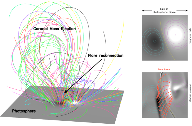
Figure 1: Eruptive flare model. [left:] Projection view of randomly plotted coronal magnetic field lines. The grayscale corresponds to the vertical component of the photospheric magnetic field $B_{z}$. [right:] Photospheric bipole viewed from above. The pink (resp. cyan) isocontours stand for positive (resp. negative) values of $B_{z}^{\mbox{\rm{\tiny max}}}/1.1,2,3,4,5$. The yellow isocontour shows the polarity inversion line $B_{z}=0$. [right-top:] The grayscale for $B_{z}$ is the same as in the left panel. [right-bottom:] The grayscale shows the vertical component of the photospheric electric currents. Strong elongated white/black patches highlight flare ribbons. The red lines show representative post-reconnection flare loops, rooted in the flare ribbons.

The MHD model was calculated in a wide numerical domain of size $20\times 20\times 30$, with a magnetic permeability $\mu=1$, using dimensionless values $B_{z}^{\mbox{\rm{\tiny max}}}=8$ in the dominant polarity, and $L^{\mbox{\rm{\tiny bipole}}}=5$. These settings resulted in a dimensionless photospheric flux inside the dominant polarity of $\phi=42$ (Aulanier et al. 2010), and a total pre-eruptive magnetic energy of $E^{\mbox{\rm{\tiny bipole}}}=225$.

Throughout the simulation, a magnetic energy of $E^{\mbox{\rm{\tiny model}}}=19\%\,E^{\mbox{\rm{\tiny bipole}}}=42$ was released. Only $5\%$ of this amount was converted into the kinetic energy of the CME. These numbers have been presented and discussed in Aulanier et al. (2012). The remaining $95\%\,E^{\mbox{\rm{\tiny model}}}$ of the magnetic energy release can then be attributed to the flare energy itself.

It must be pointed out that the simulation did not cover the full duration of the eruption. Indeed, numerical instabilities eventually prevented us from pursuing it with acceptable diffusion coefficients. Nevertheless, the rate of magnetic energy decrease had started to drop before the end of the simulation, and the electric currents within the last reconnecting field lines where relatively weak. On the one hand, this means that the total energy release $E^{\mbox{\rm{\tiny model}}}$ is expected to be slightly higher, but presumably not by much. On the other hand, the relatively low $R_{m}$ value of the simulation implies that some amount of $E^{\mbox{\rm{\tiny model}}}$ should be attributed to large-scale diffusion, rather than to the flare reconnection.

Because of these numerical concerns, we consider thereafter that the flare energy in the model was about $E=40$, but this number should not be taken as being precise. Also, within the pressureless MHD framework of the simulation, the model cannot address which part of this energy is converted into heating, and which remaining part results in particle acceleration.

It is straightforward to scale the model numbers given above into physical units. In the international system of units (SI), $\mu=4\pi 10^{-7}$, the total magnetic flux $\phi$ and the total flare energy $E$ can then be written as

$$\phi = 42\,\Bigg{(}\frac{B_{z}^{\mbox{\rm{\tiny max}}}}{8\leavevmode\nobreak\ {\mbox{\rm T}}}\Bigg{)}\,\Bigg{(}\frac{L^{\mbox{\rm{\tiny bipole}}}}{5\leavevmode\nobreak\ {\mbox{\rm m}}}\Bigg{)}^{2}\,{\mbox{\rm Wb}}\,,$$ (1)

$$E = \frac{40}{\mu}\,\Bigg{(}\frac{B_{z}^{\mbox{\rm{\tiny max}}}}{8\leavevmode\nobreak\ {\mbox{\rm T}}}\Bigg{)}^{2}\,\Bigg{(}\frac{L^{\mbox{\rm{\tiny bipole}}}}{5\leavevmode\nobreak\ {\mbox{\rm m}}}\Bigg{)}^{3}\,{\mbox{\rm J}}\,.$$ (2)

Rearranging these equations into commonly used solar units leads to:

$$\phi = 0.52\times 10^{22}\,\Bigg{(}\frac{B_{z}^{\mbox{\rm{\tiny max}}}}{{10^{3}\leavevmode\nobreak\ \mbox{\rm G}}}\Bigg{)}\,\Bigg{(}\frac{L^{\mbox{\rm{\tiny bipole}}}}{50\leavevmode\nobreak\ {\mbox{\rm Mm}}}\Bigg{)}^{2}\,{\mbox{\rm Mx}}\,,$$ (3)

$$E = 0.5\times 10^{32}\,\Bigg{(}\frac{B_{z}^{\mbox{\rm{\tiny max}}}}{{10^{3}\leavevmode\nobreak\ \mbox{\rm G}}}\Bigg{)}^{2}\,\Bigg{(}\frac{L^{\mbox{\rm{\tiny bipole}}}}{50\leavevmode\nobreak\ {\mbox{\rm Mm}}}\Bigg{)}^{3}\,{\mbox{\rm erg}}\,.$$ (4)

While the power-law dependences in these equations come from the definitions of flux and energy, the numbers themselves directly result from the MHD simulation, and not from simple order of magnitude estimates. So Eqs. (3) and (4) enable us to calculate the model predictions for a wide range of photospheric magnetic fields and bipole sizes. The results are plotted in Fig. 2. In this figure, the right vertical axis is the total sunspot area within the model, being given by $f^{-1}\,(L^{\mbox{\rm{\tiny bipole}}})^{2}$ using $f=2$. It is expressed in micro solar hemispheres (hereafter written MSH as in Baumann & Solanki 2005, although other notations can be found in the literature). Hereafter all calculated energies (resp. fluxes) will almost always be given in multiples of $10^{32}$ ergs (resp. $10^{22}$ Mx), for easier comparison between different values.

Typical decaying active regions with $L^{\mbox{\rm{\tiny bipole}}}=200$ Mm, which contain faculae of $B_{z}^{\mbox{\rm{\tiny max}}}=100$ G, have $\phi=0.8\times 10^{22}$ Mx and can produce moderate flares of $E=0.3\times 10^{32}$ ergs. Also, $\delta$-spots with $L^{\mbox{\rm{\tiny bipole}}}=40$ Mm and $B_{z}^{\mbox{\rm{\tiny max}}}=1500$ G have a lower magnetic flux $\phi=0.5\times 10^{22}$ Mx, but can produce twice stronger flares, with $E=0.6\times 10^{32}$ ergs. These energies for typical solar active regions are in good agreement with those estimated from the total solar irradiance (TSI) fluence of several observed flares (Kretzschmar 2011).

Other parameters can result in more or less energetic events. For example one can scale the model to the sunspot group from which the 2003 Halloween flares originated. Firstly, one can overplot our Fig. 1, right, onto the center of the Fig. 2 in Schrijver et al. (2006) and thus find an approximated size of the main bipole which is involved in the flare, out of the whole sunspot group. This gives a bipole size of the order of $L^{\mbox{\rm{\tiny bipole}}}\sim 65$ Mm. Secondly, observational records lead to a peak sunspot magnetic field of $B_{z}^{\mbox{\rm{\tiny max}}}=3500$ G (Livingston et al. 2012). These scalings lead to $\phi=3\times 10^{22}$ Mx and $E=13\times 10^{32}$ ergs. The modeled $\phi$ is about one third of the flux of the dominant polarity as measured in the whole active region (Kazachenko et al. 2010). Comparing this modeled flare energy $E$ with that of extreme solar flares that originated from this same active region, we find that it is twice as strong as that of the Oct 28, 2003 X17 flare (Schrijver et al. 2012), and about the same as that of the Nov 4, 2003 X28-40 flare, as can be estimated from Kretzschmar (2011) and Schrijver et al. (2012, Eq. 1).

3 Finding the upper limit on flare energy

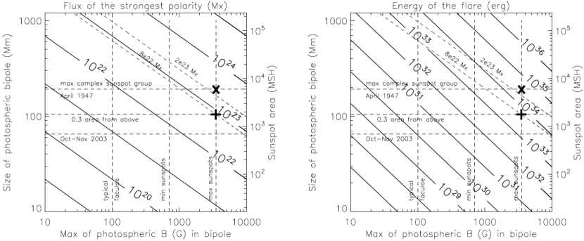
Figure 2: Magnetic flux in the dominant polarity of the bipole, and magnetic energy released during the flare, calculated as a function of the maximum magnetic field and the size of the photospheric bipole. The $\times$ and $+$ signs correspond to extreme solar values. The former is unrealistic and the latter must be very rare (see text for details).

3.1 Excluding unobserved regions in the parameter space

We indicate in Fig. 2 the minimum and maximum sunspot magnetic fields as measured from spectro-polarimetric observations since 1957. They are respectively $700$ G in the penumbra, and $3500$ G in the umbra (Solanki et al. 2006; Pevtsov et al. 2011). The latter value is an extreme that has rarely been reported in sunspot observations, and it typically is observed in association with intense flaring activity (Livingston et al. 2012).

We also indicate the maximum area of sunspot groups, including both the umbras and the penumbras. They were measured from 1874 to 1976 (Baumann & Solanki 2005) and from 1977 to 2007 (Hathaway & Choudhary 2008). These sizes follow a log-normal distribution up $3000$ MSH, but there are a few larger groups. The largest one was observed in April 1947, and its area was about $5400-6000$ MSH (Nicholson 1948; Taylor 1989). For illustration, we provide in Fig. 3 one image of this sunspot group and one of its surrounding faculae and filaments, as observed with the Meudon spectroheliograph. Interestingly, this sunspot group did not generate strong geomagnetic disturbances. This could either be due to a lack of strong enough magnetic shear in the filaments which were located between the sunspots, or to the lack of Earth-directed CMEs that could have been launched from this region. However, several other large sunspot groups, whose areas were at least $3500$ MSH, did generate major geomagnetic storms. Among those are the March 1989 event, which led to the Quebec blackout (Taylor 1989), and the December 1128 event, which produced aurorae in Asia and which corresponds to the first reported sunspot drawing (Willis & Stephenson 2001). Therefore, we conservatively keep $6000$ MSH as the maximum value. The 1874-2007 dataset does not include the first observed flare, in December 1859. Nevertheless, Hodgson (1859) reported that the size of the sunspot group associated with this event was about $96$ Mm, and one can estimate from the drawing of Carrington (1859) that its total area was smaller than $6000$ MSH.

The point marked by a thick $\times$ sign in Fig. 2 is defined by the intersection of the $3500$ G and the $6000$ MSH lines. The model states that its magnetic flux is $\phi=27\times 10^{22}$ Mx. This modeled value is much higher than $8\times 10^{22}$ Mx, which corresponds both to the dominant polarity for the Halloween flares (Kazachenko et al. 2010) and to the highest flux measured for single active regions, as observed during a sample of time-periods between 1998 and 2007 (Parnell et al. 2009). The modeled flux for this largest sunspot group is nevertheless consistent with the maximum value of $20\times 10^{22}$ Mx for an active region, as reported by Zhang et al. (2010) in a very extensive survey, ranging from 1996 to 2008. It remains difficult to estimate the highest active region flux which ever occurred. Firstly, no magnetic field measurement is available for the April 1947 sunspot group. Secondly, the automatic procedure of Zhang et al. (2010) can lead several active regions to be grouped into an apparent single region, while the method of Parnell et al. (2009) in contrast tends to fragment active region into several pieces. For reference, we therefore overplotted both $\phi=8\times 10^{22}$ and $2\times 10^{23}$ Mx values in Fig. 2.

The flare energy at the point $\times$, where the magnetic field and size of sunspot groups take their extreme values, is $E^{\times}=340\times 10^{32}$ ergs. This could a priori be considered as the maximum possible energy of a solar flare. In addition, it falls within the range of stellar superflare energies (Maehara et al. 2012). Nevertheless, we argue below that this point is unrealistic for observed solar conditions.

3.2 Taking into account the fragmentation of flux

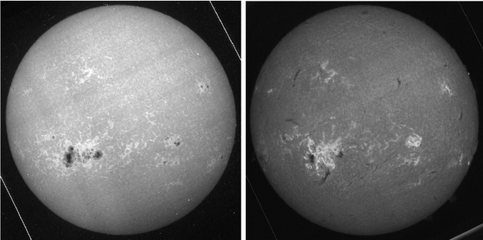
Figure 3: The largest sunspot group ever reported since the end of the nineteenth century, as observed in April 5, 1947 in Ca ii K1v (left) and H$\alpha$ (right) by the Meudon spectroheliograph.

All large sunspot groups are highly fragmented, and display many episodes of flux emergence and dispersal. We argue that this fragmentation is the reason why scaling the model to the whole area of the largest sunspot group leads to over estimate the maximum flare energy.

Firstly, sunspot groups incorporate several big sunspots, ranging from a few spots (see e.g. Schrijver et al. 2011, for February 2011) to half a dozen (see e.g. Carrington 1859; Schrijver et al. 2006, for September 1859 and October 2003 respectively) and up to more than ten (see e.g. Wang et al. 1991; Nicholson 1948, for March 1989 and April 1947 respectively; see also Fig. 3). Secondly, these groups typically have a magnetic flux imbalance (e.g. $23\%$ for the October 2003 sunspot group Kazachenko et al. 2010), because they often emerge within older active regions. This naturally creates new magnetic connections to distant regions on the Sun, in addition to possibly pre-existing ones. Thirdly, the magnetic shear tends to be concentrated along some segments only of the polarity inversion lines of a given group (Falconer et al. 2008). This is also true for the April 1947 sunspot group, as evidenced by the complex distribution of small filaments (see Fig. 3). This means that a given sunspot group is never energized as a whole. These three observational properties are actually consistent with the solar convection-driven breaking of large sub-photospheric flux tubes into a series of smaller deformed structures, as found in numerical simulations (Fan et al. 2003; Jouve et al. 2013). They show that these deformed structures should eventually emerge through the photosphere as grouped but distinct magnetic bipoles. These different bipoles should naturally possess various degrees of magnetic shear, and should not be fully magnetically connected to each other in the corona.

So both observational and theoretical arguments suggest that only a few sunspots from a whole sunspot group should be involved in a given flare. Unfortunately, the fraction of area to be considered, and to be compared with the size of the bipole in the model, is difficult to estimate.

We consider the Oct-Nov 2003 flares, for example. Our estimation of $L^{\mbox{\rm{\tiny bipole}}}\sim 65$ Mm, as given above, results in a modeled sunspot area of $700$ MSH (see Fig. 2). This is about $27\%$ of the maximum area measured for the whole sunspot group, which peaked at $2600$ MSH on Oct 31. Another way to estimate this fraction is to measure the ratio between the magnetic flux swept by the flare ribbons, and that of the whole active region. Qiu et al. (2007) and Kazachenko et al. (2012) reported a ratio of $25\%$ and $31\%$ for the Oct 28 flare, respectively. The same authors also reported on a dozen of other events, for which one can estimate ratios ranging between $10\%$ and $30\%$, on average.

These considerations lead us to conjecture that $30\%$ at most of the area of the largest observed sunspot group, as reported by Nicholson (1948) and Taylor (1989), i.e. a maximum of $1800$ MSH, can be involved in a flare. This is more than $2.5$ times the area of the bipole involved in the Halloween flares. In Fig. 2, we therefore plot another point indicated by a thick $+$ sign, located at the intersection of the $3500$ G and the $1800$ MSH lines. In the model, this corresponds to $L^{\mbox{\rm{\tiny bipole}}}=105$ Mm. The flare energy at this point is $E^{+}=56\times 10^{32}$ ergs. Under the assumptions of the model, and considering that it probably corresponds to the most extreme observed solar conditions, $E^{+}$ should correspond to the upper limit on solar flare energy.

3.3 Numerical concerns

As for all numerical models, various limitations could play a role in changing the estimated maximum flare energy $E^{+}$.

We mentioned above that the simulation did not cover the duration of the full eruption, because some numerical instabilities eventually developed. On the one hand, this means that our flare energies are slightly under estimated. But on the other hand, the low $R_{m}$ must lead to a weak large-scale diffusion. It should not be very strong, however, since the characteristic diffusion time at the scale of the modeled bipole can be estimated as $150$ times the duration of the simulation. Still, it ought to take away some fraction of the magnetic energy released during the simulation, so that our flare energies are slightly over estimated. Quantifying the relative importance of both effects is unfortunately hard to achieve.

Moreover, applying different spatial distribution of shear during the pre-flare energy storage phase could lead to a different amount of energy release (Falconer et al. 2008). But in our model, the shearing motions were extended all along the polarity inversion line in the middle of the flux concentrations. Therefore we argue that it will be difficult for different settings to produce significantly higher flare energies.

Another concern is that our simulation produces a CME kinetic energy which is only $5\%$ of the flare energy. But current observational energy estimates imply that the kinetic energy of a CME can be the same as (Emslie et al. 2005) and up to three times higher than (Emslie et al. 2012) the bolometric energy of its associated flare. This strong discrepancy cannot be attributed to the fact that our simulation was limited in time. Indeed, other 3D (resp. 2.5D) MHD models calculated by independent groups and codes predict that no more than $10\%$ (resp. $30\%$) of the total released magnetic energy is converted into the CME kinetic energy (Amari et al. 2003; Jacobs et al. 2006; Lynch et al. 2008; Reeves et al. 2010). This means that it is unclear whether the relatively weaker CME kinetic energy in our model should be attributed to observational biases, or to numerical problems commonly shared by several groups and codes.

In principle, the validity of the model can also be questioned because magnetic reconnection is ensured by resistivity, with a relatively low magnetic Reynolds number $R_{m}$ as compared to that of the solar corona. This may lead to different reconnection rates from those found in collisionless reconnection simulations (see e.g. Aunai et al. 2011). The reconnection rate is indeed important for the flare energy release in fully three-dimensional simulations of solar eruptions. In principle, slower (resp. faster) reconnection releases weaker (resp. larger) amounts of magnetic energy per unit time. Nevertheless, one might argue that the time-integrated energy release, during the whole flare, could be not very sensitive to the reconnection rate. However the energy content which is available at a given time, within a given pair of pre-reconnecting magnetic field lines, strongly depends on how much time these field lines have had to stretch ideally (as described in Aulanier et al. 2012), and thus by how much their magnetic shear has decreased before they reconnect. This explains why the time-evolution of the eruption makes the reconnection rate important for time-integrated energy release. In our simulation, we measure the reconnection rate from the average Mach number $M$ of the reconnection inflown. During the eruption, it increases in time from $M\sim 0.05$ to $M\sim 0.2$ approximately. These reconnection rates are fortunately comparable to those obtained for collisionless reconnection. So we conjecture that the limited physics inside our modeled reconnecting current sheet should not have drastic consequences for the flare energies. Nevertheless, it should be noted that this result probably does not hold for other resistive MHD simulations that use very different $R_{m}$.

We foresee that these numerical concerns are probably not extremely sensitive: the orders of magnitudes that we find for flare energies are likely to be correct. But it is difficult at present to assert that we estimate flare energies with a precision better than several tens of percents, or even more. Therefore we conservatively round up the upper value $E^{+}$ to $6\times 10^{33}$ ergs. In the future, data-driven simulations which can explore the parameter space and which incorporate more physics will have to be developed to fine-tune the present analyses.

4 Summary and discussion

So as to estimate the maximum possible energy of solar flare, we used a dimensionless numerical 3D MHD simulation for solar eruptions (Aulanier et al. 2010, 2012). We had previously shown that this model successfully matches the observations of active region magnetic fields, of coronal sigmoids, of flare ribbons and loops, of CMEs, and of large-scale propagation fronts.

We scaled the model parameters to physical values. Typical solar active region parameters resulted in typically observed magnetic fluxes (Parnell et al. 2009; Zhang et al. 2010) and flare energies (Kretzschmar 2011; Schrijver et al. 2012). We then scaled the model using the largest measured sunspot magnetic field (Solanki et al. 2006), and the area of the largest sunspot group ever reported, which developed in March-April 1947 (Nicholson 1948; Taylor 1989).

In addition, we took into account that observations show that large sunspots groups are always fragmented into several spots, and are never involved in a given flare as a whole. This partitioning can presumably be attributed to sub-photospheric convective motions. Since those motions are always present because of the solar internal structure (Brun & Toomre 2002), it is difficult to imagine that the Sun will ever produce a large sunspot group consisting of a single pair of giant sunspots. Based on some approximated geometrical and reconnected magnetic flux estimations, we considered that only $30\%$ the area of a given sunspot group can be involved in a flare.

Keeping in mind the assumptions and limitations of the numerical model, these scalings resulted in a maximum flare energy of $\sim 6\times 10^{33}$ ergs. This is is ten times the energy of the Oct 28, 2003 X17 flare, as reported in Schrijver et al. (2012). In addition, this value is about six times higher than the maximum energy in TSI fluence that can be estimated from the SXR fluence of the Nov 4, 2003 X28-40 flare, using the scalings given by Kretzschmar (2011) and Schrijver et al. (2012). Finally, it lies in the energy range of the weakest superflares that were reported by Maehara et al. (2012) for numerous slowly-rotating and isolated Sun-like stars. But it is several orders of magnitude smaller than that of strong stellar superflares.

One could ask what the frequency is at which the Sun can produce a maximum flare like this. Observational records since 1874 reveal that the area of sunspot groups follow a sharp log-normal distribution (Baumann & Solanki 2005; Hathaway & Choudhary 2008). Unfortunately, the statistics for sunspot groups larger than $3000$ MSH in area are too poor to estimate whether or not this distribution is valid up to $6000$ MSH. In addition, neither do all active regions or sunspot groups generate flares, nor do they always generate them at the maximum energy, as calculated by the model. The reason must be that a solar eruption requires a strong magnetic sheared polarity inversion line, and current observations show that this does not occur in all solar active regions (Falconer et al. 2008). Consequently it is currently difficult to estimate the probability of appearance of the strongest flare that we found. We can only refer to Baumann & Solanki (2005) and Hathaway & Choudhary (2008), who reported that the size of sunspot groups follows a clear log-normal distribution up to $3000$ MSH, and to Cliver & Svalgaard (2004) and Schrijver et al. (2012), who argue that this upper limit on flare energy was never reached in any observed solar flare since, even including the Carrington event of Sept 1859.

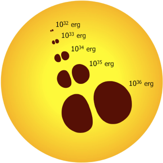
Figure 4: Schematic representation of several modeled sunspot pairs on the solar disk, with their corresponding modeled flare energies. Note that our estimations state that in the real Sun, a given pair will often be embedded in a much larger sunspot group, from which only the bipole that is shown here will be involved in the flare.

When the model is scaled to the strongest measured sunspot magnetic field, i.e. 3.5 kG, it can be used to calculate the size of the sunspot pair that is required to generate the solar flares of various energies. We plot those in Fig. 4. These scalings can also be used to relate stellar superflares to starspot sizes. But it should be noted that starspot magnetic fields are still difficult to measure reliably, and that current estimates put them in the range of $2-5$ kG (Berdyugina 2005). With these scalings, a superflare of $10^{36}$ ergs requires a very large single pair of spots, whose extent is $48^{\circ}$ in longitude/latitude, at the surface of a Sun-like star. While such spots have been observed indirectly in non-Sun-like stars as well as in young fast-rotating Sun-like stars (Berdyugina 2005; Strassmeier 2009), they have never been reported on the Sun.

5 Conclusion

We combined a numerical magnetohydrodynamic model for solar eruptions calculated with the OHM code and historical sunspot observations starting from the end of the nineteenth century. We concluded that the maximum energy of solar flares is about six times that of the strongest-ever directly-observed flare of Nov 4, 2003.

One unaddressed question is whether or not the current solar convective dynamo can produce much larger sunspot groups, as required to produce even stronger flares according to our results. This seems unlikely, since such giant sunspot groups “have not been recorded in four centuries of direct scientific observations and in millennia of sunrises and sunsets viewable by anyone around the world”, to quote Schrijver et al. (2012). It can thus reasonably be assumed that, during the most recent few billion years while on the main sequence, the Sun never has produced, and never will produce, a flare more energetic than this upper limit. We thus conjecture that one condition for Sun-like stars to produce superflares is to host a dynamo that is much stronger than that of an aged Sun with a rotation rate exceeding several days.

On the one hand, our results suggest that we have not experienced the largest possible solar flare. But on the other hand, and unless the dynamo theory proves otherwise, our results also provide an upper limit for extreme space weather conditions, that does not exceed those related to past observed flares by much.