Continuous wave solutions in spinor Bose-Einstein condensates

Abstract

We find analytic continuous wave (cw) solutions for spinor Bose-Einstein condensates (BECs) in a magnetic field that are more general than those published to date. For particles with spin $F=1$ in a homogeneous one-dimensional trap, there exist cw states in which the chemical potential and wavevectors of the different spin components are different from each other. We include linear and quadratic Zeeman splitting. Linear Zeeman splitting, if the magnetic field is constant and uniform, can be mathematically eliminated by a gauge transformation, but quadratic Zeeman effects modify the cw solutions in a way similar to non-zero differences in the wavenumbers between the different spin states. The solutions are stable fixed points within the continuous wave framework, and the coherent spin mixing frequencies are obtained.

I Introduction

Atomic Bose-Einstein condensates (BECs) with nonvanishing total angular momentum have been experimentally obtained, in which the BECs contain several spin components, i.e., they are spinor BECs. Examples are $H$ (with total spin $F=0$ and $F=1$) Fried.1998 , ⁷Li ($F=1$, $F=2$; note that the scattering length is negative, making the BEC self-attractive) Bradley.1995 ; Bradley.1997 , ²³Na ($F=1$, $F=2$) Simkin.1999 , ³⁹K ($F=1$, $F=2$; scattering length has a small negative value) Roati.2007 , ⁴¹K ($F=1$, $F=2$) Modugno.2001 , ⁵²Cr ($F=3$; with a large magnetic moment) Griesmaier.2005 ; Beaufils.2008 , ⁸⁵Rb ($F=2$, $F=3$; negative scattering length), ⁸⁷Rb ($F=1$, $F=2$) Barrett.2001 ; Chang.2004 ; Sadler.2006 ; Leslie.2009 , ¹³³Cs ($F=3$, $F=4$) Weber.2003 , ¹⁶⁴Dy ($F=8$) Lu.2011 , and ¹⁶⁸Er ($F=6$) Aikawa.2012 . When a BEC is held in a magnetic trap, only spin components of one sign are trapped, often leaving just one spin orientation. An optical trap, however, may hold all spin components of a given hyperfine state. In this case, the spinor character is important, and a scalar model of a BEC is insufficient. Optical traps for spinor BECs are now common, and there is work on creating BECs using only optical traps Barrett.2001 ; Beaufils.2008 . Optical traps have also been created in the form of a closed ring Gupta.2005 ; Olson.2007 ; Lesanovsky.2007 ; Henderson.2009 ; Ryu.2007 .

The spinor properties of BECs have been the focus of recent theoretical and experimental research Ueda.2012 ; KawaguchiUeda.2012 , especially ²³Na, ⁸⁷Rb, and ⁵²Cr. The spinor properties of a BEC can critically affect the dynamics: The spinor character of BECs underlies the formation of domain walls (transition regions, which may be stable or unstable, between distinct spin domains) and vortices Sadler.2006 ; Saito.2007 ; Lamacraft.2007 . Oscillatory coherent spin mixing occurs in spinor BECs Zhang.2005 ; Gerbier.2006 . Spinor BECs are subject to modulational (Benjamin-Feir) instabilities Robins.2001 ; Konotop.2002 ; Li.2005 ; KawaguchiUeda.2012 even when the nonlinearity is repulsive, whereas scalar BECs are not. Spinor BECs support a variety of soliton solutions that are not found in scalar BECs IedaMiyakawaWadati.2004 ; WadatiTsuchida.2006 ; UchiyamaIedaWadati.2006 ; SzankowskiTrippenbachInfeldRowlands.2010 ; SzankowskiTrippenbachInfeldRowlands.2011 .

Here we study continuous wave (cw) [plane wave] solutions of $F=1$ spinor BEC condensates. Section II introduces the model, which includes spin-dependent and spin-independent mean-field effects, and linear and quadratic Zeeman effects (but does not include spin-dipolar effects, which can be important, e.g., in ⁵²Cr). Section III derives the most general possible cw solutions for $F=1$ spinor BECs on a homogeneous background with a homogeneous magnetic field. This section gives, even before inclusion of the linear and quadratic Zeeman effects, more general families of cw solutions than have heretofore been published. Section IV contains a summary and conclusions.

II Quantitative model for spinor BECs with magnetic fields

The Hamiltonian density for an $F=1$ spinor BEC with linear and quadratic Zeeman effect (and without significant spin-dipolar coupling) is OhmiMachida.1998 ; Ho.1998

$$\mathcal{H} = \frac{\hbar^{2}}{2m}\mathbf{\nabla}\Phi_{a}^{\dagger}\cdot\mathbf{\nabla}\Phi_{a}+\frac{c_{0}}{2}\Phi_{a}^{\dagger}\Phi_{b}^{\dagger}\Phi_{b}\Phi_{a}+\frac{c_{2}}{2}\Phi_{a}^{\dagger}\Phi_{a^{\prime}}^{\dagger}\mathbf{F}_{ab}\cdot\mathbf{F}_{a^{\prime}b^{\prime}}\Phi_{b^{\prime}}\Phi_{b}-pB\Phi_{a}^{\dagger}\mathbf{F}_{ab}^{z}\Phi_{b}+qB^{2}\Phi_{a}^{\dagger}(\mathbf{F}_{ab}^{z})^{2}\Phi_{b},$$ (1)

where $\mathbf{\Phi}=(\phi_{1},\phi_{0},\phi_{-1})^{\mathrm{t}}$ is a vector with the amplitudes of the $M_{F}=1$ component (spin in the same direction as the magnetic field), $M_{F}=0$, and $M_{F}=-1$; $m$ is the mass of the atom, $c_{0}$ and $c_{2}$ are the coefficients of the spin-independent and spin-dependent parts of the mean-field; $c_{0}$ gives rise to self-phase modulation and $c_{2}$ is the spin-dependent mean-field coefficient which also gives rise to phase modulation, and parametric nonlinearity. $\mathbf{F}$ is a vector in which each component is a 3$\times$3 spin-1 matrix, i.e., the dimensionless spin vector $\mathbf{F}$ has components,

$$F_{x}=\frac{1}{\sqrt{2}}\left(\!\!{\begin{array}[]{ccc}0&1&0\\ 1&0&1\\ 0&1&0\end{array}}\!\!\right),\quad F_{y}=\frac{1}{\sqrt{2}}\left(\!\!{\begin{array}[]{ccc}0&{-i}&0\\ i&0&{-i}\\ 0&i&0\end{array}}\!\!\right),\quad F_{z}=\left(\!\!{\begin{array}[]{ccc}1&0&0\\ 0&0&0\\ 0&0&{-1}\end{array}}\!\!\right).$$ (2)

The magnetic field ${\bf B}$ is taken to be constant and uniform and in the $z$-direction, ${\bf B}=B\hat{\mathbf{z}}$, and $p$ and $q$ are linear and quadratic Zeeman coefficients Saito.2007 ; Lamacraft.2007 ; Zhang.2005 . If the BEC is confined to one dimension (by a strong optical trap in the transverse directions), the Hamiltonian gives the following governing equations for the BEC:

$$i\hbar\frac{\partial}{\partial t}\phi_{1} = -\frac{\hbar^{2}}{2m}\frac{\partial^{2}}{\partial z^{2}}\phi_{1}+c_{0}\left(|\phi_{1}|^{2}+|\phi_{0}|^{2}+|\phi_{-1}|^{2}\right)\phi_{1}$$ (3a)

$$+c_{2}\left[\left(|\phi_{1}|^{2}+|\phi_{0}|^{2}-|\phi_{-1}|^{2}\right)\phi_{1}+\phi_{0}^{2}\phi_{-1}^{*}\right]+(-pB+qB^{2})\phi_{1}\,,$$

$$i\hbar\frac{\partial}{\partial t}\phi_{0} = -\frac{\hbar^{2}}{2m}\frac{\partial^{2}}{\partial z^{2}}\phi_{0}+c_{0}\left(|\phi_{1}|^{2}+|\phi_{0}|^{2}+|\phi_{-1}|^{2}\right)\phi_{0}$$ (3b)

$$+c_{2}\left[\left(|\phi_{1}|^{2}+|\phi_{-1}|^{2}\right)\phi_{0}+2\phi_{1}\phi_{0}^{*}\phi_{-1}\right]\,,$$

$$i\hbar\frac{\partial}{\partial t}\phi_{-1} = -\frac{\hbar^{2}}{2m}\frac{\partial^{2}}{\partial z^{2}}\phi_{-1}+c_{0}\left(|\phi_{1}|^{2}+|\phi_{0}|^{2}+|\phi_{-1}|^{2}\right)\phi_{-1}$$ (3c)

$$+c_{2}\left[\left(-|\phi_{1}|^{2}+|\phi_{0}|^{2}+|\phi_{-1}|^{2}\right)\phi_{-1}+\phi_{0}^{2}\phi_{1}^{*}\right]+(pB+qB^{2})\phi_{-1}\,.$$

Time and space are denoted by $t$ and $z$, respectively. The system has Galilean invariance. Materials with negative $c_{2}$ are ferromagnetic, since with $c_{2}<0$, at a given particle density and at zero magnetic field, the energy density is lower when the local BEC is in a pure spin state $M_{F}=1$ or $M_{F}=-1$, than in a state composed of a mixture of spins $M_{F}=1$ and $M_{F}=-1$. The BEC prefers to have a non-zero net spin locally. Materials with positive $c_{2}$ are antiferromagnetic, or polar, since with $c_{2}<0$, at a given particle density and without a magnetic field, the energy density is lower when the local BEC is 50% $M_{F}=1$ and 50% $M_{F}=-1$. The BEC prefers to be in a state where opposite spins balance each other exactly and, cancel out in the total magnetic moment. The nonlinear coefficients, which are proportional to the s-wave scattering lengths $a_{0}$, $a_{2}$ for the total spin $F=0$ and $F=2$ channels, $g_{0}=(4\pi\hbar^{2}/m)a_{0}$, $g_{2}=(4\pi\hbar^{2}/m)a_{2}$, with the nonlinear coefficients in the governing equations above given by $c_{0}=(g_{0}+2g_{2})/3$, $c_{2}=-(g_{0}-g_{2})/3$. If the BEC is confined to one dimension, the values of the nonlinear coefficients are modified as discussed in Refs. Olshanii.1998 ; Bergeman.2003 . For ⁸⁷Rb, the scatterings lengths are $a_{0}=101.8\,a_{B}$ and $a_{2}=a_{0}-1.45\,a_{B}$, where $a_{B}$ is the Bohr radius Chang.2005 ; KlausenBohnGreene.2001 ; KempenKokkelmansHeinzenVerhaar.2002 . This gives ⁸⁷Rb a negative $c_{2}$, which makes it ferromagnetic. For ²³Na, the scattering lengths have been measured to be $a_{0}=50.0\,a_{B}$, $a_{2}=a_{0}+5.0\,a_{B}$. ²³Na has a positive $c_{2}$, so it is antiferromagnetic, or “polar.” The masses of the two atoms are $m_{\mathrm{Rb}}=1.4192\times 10^{-22}$g, $m_{\mathrm{Na}}=3.817\times 10^{-23}$g. In bulk, these yield $c_{0}(\mathrm{Rb})=5.26\times 10^{-38}$ erg cm³, $c_{2}(\mathrm{Rb})=-2.52\times 10^{-40}$ erg cm³ and $c_{0}(\mathrm{Na})=10.33\times 10^{-38}$ erg cm³, $c_{2}(\mathrm{Na})=3.23\times 10^{-39}$ erg cm³; the rations $c_{2}/c_{0}$ are $-0.0048$ for ⁸⁷Rb and $0.0313$ for ²³Na. The quadratic Zeeman coefficient is $q=h\times 575$ Hz/G² for ⁸⁷Rb, and $q=h\times 70$ Hz/G² for ²³Na. Equations (3) are integrable when $c_{2}=0$ (in which case the system is a set of generalized Manakov equations Nakkeeran.1998 ; Manakov.1973 ) or $c_{2}=c_{0}$ IedaMiyakawaWadati.2004 ; WadatiTsuchida.2006 ; IedaWadati.2007 .

The linear Zeeman splitting can be eliminated from the governing equations (3) by the change of variables (i.e., the gauge transformation) $\phi_{1}\equiv\psi_{1}\exp[i(pB/\hbar)t]$, $\phi_{0}\equiv\psi_{0}$, $\phi_{-1}\equiv\psi_{-1}\exp[-i(pB/\hbar)t]$. Let us take this as done, but retain the same variable names as previously, to avoid excessive complicated notation. Because the linear Zeeman splitting can be eliminated by this gauge transformation, the analysis of the nil linear Zeeman splitting, $p=0$, can equally well describe the case with non-zero linear Zeeman splitting. Generally, analyses should either make use of this gauge transformation or not force all the spin components to have the same frequency (chemical potential), or one may erroneously impose restrictions that do not exist in the physics. Quadratic Zeeman splitting cannot be eliminated by a change of variables.

The analysis below is in terms of infinite continuous (plane) waves. It applies equally to waves with periodic boundary conditions, either physical ones due to the BECs existing in a circular trap Gupta.2005 ; Olson.2007 ; Lesanovsky.2007 ; Henderson.2009 ; Ryu.2007 , or theoretical ones due to the need to limit the numerical domain. Periodic boundary conditions quantize the wavenumbers.

The governing equations (3) can be non-dimensionalized by the change of variables

$$t^{\prime} = t/t_{d},$$ (4a)

$$z^{\prime} = z/z_{d}=z/\sqrt{\hbar t_{d}/m},$$ (4b)

$$\phi_{j}^{\prime} = \phi_{j}/\phi_{d}=\phi_{j}/\sqrt{\hbar/(c_{0}t_{d})}.$$ (4c)

In dimensionless variables (4c), the governing equations (3) take the same form but with $\hbar\rightarrow 1$, $m\rightarrow 1$, $c_{0}\rightarrow 1$, and $c_{2}\rightarrow c_{2}/c_{0}$. The physical frequencies and wavenumbers are equal to the dimensionless quantities times $t_{d}^{-1}$ and $z_{d}^{-1}=(\sqrt{\hbar t_{d}/m})^{-1}$, respectively. The physical amplitudes of the BEC are the dimensionless ones times $\sqrt{\hbar/(c_{0}t_{d})}$. The physical energy is equal to the dimensionless energy multiplied by $\hbar/t_{d}$, and the physical energy is the dimensionless quantity times $\hbar^{-1/2}m^{3/2}t_{d}^{-5/2}$. We will use the dimensionless variables in the figures in order to emphasize the generality, but retain the dimensions in the body of the text.

The Lagrangian density that gives Eqs. (3) is

$$\mathcal{L} = \frac{i\hbar}{2}(\phi_{1}^{*}\phi_{1,t}-\phi_{1}\phi_{1,t}^{*}+\phi_{0}^{*}\phi_{0,t}-\phi_{0}\phi_{0,t}^{*}+\phi_{-1}^{*}\phi_{-1,t}-\phi_{-1}\phi_{-1,t}^{*})$$ (5)

$$- \frac{\hbar^{2}}{2m}(|\phi_{1,z}|^{2}+|\phi_{0,z}|^{2}+|\phi_{-1,z}|^{2})-\frac{c_{0}}{2}\left(|\phi_{1}|^{2}+|\phi_{0}|^{2}+|\phi_{-1}|^{2}\right)^{2}$$

$$- c_{2}\left[\frac{1}{2}\left(|\phi_{1}|^{2}-|\phi_{-1}|^{2}\right)^{2}+|\phi_{0}|^{2}\left(|\phi_{1}|^{2}+|\phi_{-1}|^{2}\right)+\phi_{1}^{*}\phi_{0}^{2}\phi_{-1}^{*}+\phi_{1}\phi_{0}^{*2}\phi_{-1}\right]-qB^{2}(|\phi_{1}|^{2}+|\phi_{-1}|^{2})\,,$$

and the Hamiltonian density is

$$\mathcal{H} = \frac{\hbar^{2}}{2m}(|\phi_{1,z}|^{2}+|\phi_{0,z}|^{2}+|\phi_{-1,z}|^{2})+\frac{c_{0}}{2}\left(|\phi_{1}|^{2}+|\phi_{0}|^{2}+|\phi_{-1}|^{2}\right)^{2}$$ (6)

$$+ c_{2}\left[\frac{1}{2}\left(|\phi_{1}|^{2}-|\phi_{-1}|^{2}\right)^{2}+|\phi_{0}|^{2}\left(|\phi_{1}|^{2}+|\phi_{-1}|^{2}\right)+\phi_{1}^{*}\phi_{0}^{2}\phi_{-1}^{*}+\phi_{1}\phi_{0}^{*2}\phi_{-1}\right]+qB^{2}(|\phi_{1}|^{2}+|\phi_{-1}|^{2})\,.$$

If any two of the three spin fields are zero, then the remaining field is governed by a simple nonlinear Schrödinger equation, which is completely integrable ZakharovShabat.1971 ; ZakharovShabat.1973 . If the $M_{F}=0$ field is nil ($\phi_{0}=0$), then the $M_{F}=\pm 1$ fields ($\phi_{1}$, $\phi_{-1}$) are governed by a pair of coupled nonlinear Schrödinger equations,

$$i\hbar\frac{\partial}{\partial t}\phi_{1} = -\frac{\hbar^{2}}{2m}\frac{\partial^{2}}{\partial z^{2}}\phi_{1}+\left[(c_{0}+c_{2})|\phi_{1}|^{2}+(c_{0}-c_{2})|\phi_{-1}|^{2}\right]\phi_{1}\,,$$ (7a)

$$i\hbar\frac{\partial}{\partial t}\phi_{-1} = -\frac{\hbar^{2}}{2m}\frac{\partial^{2}}{\partial z^{2}}\phi_{-1}+\left[(c_{0}-c_{2})|\phi_{1}|^{2}+(c_{0}+c_{2})|\phi_{-1}|^{2}\right]\phi_{-1}\,.$$ (7b)

The coupled nonlinear Schrödinger equations have been intensely studied (see, e.g., Ref. Yang.2010 ). This case is completely integrable if and only if $c_{2}=0$, $c_{0}=c_{2}$, or $c_{0}=0$ ZakharovSchulman.1982 . Depending on the coefficients, there may be bright soliton solutions Manakov.1973 ; Agrawal.2001 , dark soliton solutions KivsharTuritsyn.1993 , bright-dark soliton solutions RadhakrishnanLakshmanan.1995 ; RadhakrishnanLakshmananDaniel.1995 , and domain wall solutions HaeltermanSheppard.1994 ; Malomed.1994 . We will concentrate less on this limit, and more on aspects of spinor BECs that do not overlap with the thoroughly studied coupled nonlinear Schrödinger equations.

III Continuous wave solutions

Continuous waves (cws) are the simplest shapes, so cw solutions are where analysis of the system should begin. The most general cw is

$$\phi_{1} = A_{1}\exp[i(\theta_{1}+k_{1}z-\omega_{1}t)]\,,$$ (8a)

$$\phi_{0} = A_{0}\exp[i(\theta_{0}+k_{0}z-\omega_{0}t)]\,,$$ (8b)

$$\phi_{-1} = A_{-1}\exp[i(\theta_{-1}+k_{-1}z-\omega_{-1}t)]\,,$$ (8c)

where the parameters are real-valued and, without loss of generality, $A_{1}$, $A_{0}$, $A_{-1}$ are positive definite. Note that this is more general than the cw ansatz in Ref. WadatiTsuchida.2006 , in that the frequencies and wavenumbers need not all be the same. The analysis herein shows that there exist a wider range of cw solutions than, for example, in Ref. WadatiTsuchida.2006 . Put the trial function (8) into Eqs. (3).

If $c_{2}=0$, then Eqs. (3) are a generalized Manakov system Manakov.1973 , but with three fields rather than two. This limiting case is completely integrable Nakkeeran.1998 . There are cw solutions for every value of the amplitude ($A_{j}$), wavenumber ($k_{j}$), and phase ($\theta_{j}$). The frequencies of the fields are

$$\hbar\omega_{j}=\frac{\hbar^{2}k_{j}^{2}}{2m}+c_{0}(A_{1}^{2}+A_{0}^{2}+A_{-1}^{2})\,.$$ (9)

If $c_{2}\neq 0$, then the parametric term requires a relation between the phases of the three fields,

$$k_{0} = \frac{1}{2}(k_{1}+k_{-1})\,,$$ (10a)

$$\omega_{0} = \frac{1}{2}(\omega_{1}+\omega_{-1})\,,$$ (10b)

$$\theta_{0} = \frac{1}{2}(\theta_{1}+\theta_{-1}+n\pi)\,,$$ (10c)

where $n$ is an integer. The equations for the magnitudes of the fields are

$$\hbar\omega_{1} = \frac{\hbar^{2}k_{1}^{2}}{2m}+c_{0}\left(A_{1}^{2}+A_{0}^{2}+A_{-1}^{2}\right)+c_{2}\left[A_{1}^{2}+A_{0}^{2}-A_{-1}^{2}+(-1)^{n}A_{0}^{2}A_{-1}/A_{1}\right]+qB^{2}A_{1}\,,$$ (11a)

$$\hbar\omega_{0} = \frac{\hbar^{2}k_{0}^{2}}{2m}+c_{0}\left(A_{1}^{2}+A_{0}^{2}+A_{-1}^{2}\right)+c_{2}\left[A_{1}^{2}+A_{-1}^{2}+2(-1)^{n}A_{1}A_{-1}\right]\,,$$ (11b)

$$\hbar\omega_{-1} = \frac{\hbar^{2}k_{-1}^{2}}{2m}+c_{0}\left(A_{1}^{2}+A_{0}^{2}+A_{-1}^{2}\right)+c_{2}\left[-A_{1}^{2}+A_{0}^{2}+A_{-1}^{2}+(-1)^{n}A_{0}^{2}A_{1}/A_{-1}\right]+qB^{2}A_{-1}\,.$$ (11c)

Equations (11) and (10b) give a formula for the magnitude $A_{0}$ of mode $\phi_{0}$,

$$A_{0}^{2}=2(-1)^{n}A_{1}A_{-1}\left(1-\frac{(\hbar^{2}/2m)[(k_{1}-k_{-1})/2]^{2}+qB^{2}}{c_{2}[A_{1}+(-1)^{n}A_{-1}]^{2}}\right)\,.$$ (12)

For a cw solution to exist, $A_{0}$ must be non-negative, as per ansatz (8), so its square must be non-negative, $A_{0}^{2}\geq 0$. The ranges in which the different cw solutions exist depends on the magnitude and sign of the quantity $[\hbar^{2}(k_{1}-k_{-1})^{2}/8m+qB^{2}]/c_{2}$. If the quadratic Zeeman coefficient is non-negative ($q\geq 0$), the sign of this is either zero or equal to the sign of $c_{2}$. If the quadratic Zeeman coefficient is negative ($q<0$), a sufficiently strong magnetic field can change the sign of the quantity. For particles with $F=1$, the quadratic Zeeman coefficient is normally positive, $q>0$. (Particles with $F=2$, normally have negative quadratic Zeeman coefficients, $q<0$.) The sign and magnitude of $q$ can be changed, however, by using the alternating current Stark shift with microwave radiation Leslie.2009 ; Gerbier.2006 ; Ueda.2012 . We will refer to $[\hbar^{2}(k_{1}-k_{-1})^{2}/8m+qB^{2}]/c_{2}>0$ as the generalized antiferromagnetic case, and $[\hbar^{2}(k_{1}-k_{-1})^{2}/8m+qB^{2}]/c_{2}<0$ as the generalized ferromagnetic case. In the generalized antiferromagnetic case, there are cw solutions with even $n$ (which we will denote by $n=0$ in the labels below) when

$$(A_{1}+A_{-1})^{2}\geq\frac{1}{c_{2}}\left[\frac{\hbar^{2}}{2m}\left(\frac{k_{1}-k_{-1}}{2}\right)^{2}+qB^{2}\right]\,,$$ (13)

and there are cw solutions with odd $n$ (which we will denote by $n=1$) when

$$0<(A_{1}-A_{-1})^{2}\leq\frac{1}{c_{2}}\left[\frac{\hbar^{2}}{2m}\left(\frac{k_{1}-k_{-1}}{2}\right)^{2}+qB^{2}\right]\,.$$ (14)

There are no $n=1$ type cw solutions when $A_{1}=A_{-1}$ because the difference of the amplitudes in the denominator of Eq. (12) makes the value of $A_{0}$ go to infinity as $(A_{1}-A_{-1})$ approaches zero. In the generalized ferromagnetic case, there are $n=0$ cw solutions for all values of the spin $M_{F}=0$ and spin $M_{F}=-1$ magnitudes ($A_{1},A_{-1}\in{\cal R}^{\geq 0}$). The generalized ferromagnetic case does not support any $n=1$ type cw solutions. Recall that there exist cw solutions with vanishing $M_{F}=0$ BEC fields for any values of the $M_{F}=\pm 1$ BEC magnitudes, whether the BEC is ferromagnetic or antiferromagnetic. This existence ranges are summarized in Table 1 and in Fig. 1.

$x\equiv[\hbar^{2}(k_{1}-k_{-1})^{2}/8m+qB^{2}]/c_{2}$	cw (CNLS)	cw ($n=0$)	cw ($n=1$)
$>0$	$A_{1},A_{-1}\in{\cal R}^{\geq 0}$	$(A_{1}+A_{-1})^{2}\geq x$	$0<(A_{1}-A_{-1})^{2}\leq x$
$\leq 0$	$A_{1},A_{-1}\in{\cal R}^{\geq 0}$	$A_{1},A_{-1}\in{\cal R}^{\geq 0}$	No solutions.

Table 1: Existence ranges of the three possible cw solutions, for different values of the spin-dependent nonlinear coefficient $c_{2}$, particle mass $m$, quadratic Zeeman coefficient $q$, magnetic field $B$, and given difference in the wavenumbers between the $M_{F}=\pm 1$ spin components. The allowed magnitudes of the amplitudes of the fields for the BEC with spin $M_{F}=\pm 1$ are denoted by $A_{\pm 1}$, as in the ansatz (8), and the magnitude of the amplitudes of the BEC with spin $M_{F}=0$ is either $0$ (“CNLS”) or goes according to the formula (12).

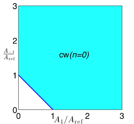
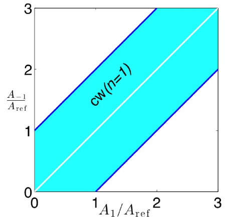
Figure 1: (Color online) Existence ranges of the cw solutions in spinor BECs in the generalized antiferromagnetic case ($A_{\mathrm{ref}}\equiv[\hbar^{2}(k_{1}-k_{-1})^{2}/8m+qB^{2}]/c_{2}\geq 0$; note that in the most familiar cw solutions, with $k_{1}=k_{0}=k_{-1}$ and zero quadratic Zeeman splitting, $A_{\mathrm{ref}}=0$; in this limit, the $n=0$ cw solutions have $A_{0}=\sqrt{2A_{1}A_{-1}}$ and exist for all values of the particle densities $M_{F}=\pm 1$, and the $n=1$-type cw does not exist). Part (a) shows cws with relative phase of the $M_{F}=0$ field corresponding to even $n$ in the trial function Eq. (8), with $\theta_{1}+\theta_{-1}-2\theta_{0}=n\pi$. Part (b) shows the cws with relative phase designated by odd $n$. For odd $n$, the particle density of the $M_{F}=0$ field approaches infinity as the densities of $M_{F}=1$ and $M_{F}=-1$ fields approach equality.

The Hamiltonian density of the cw solutions is

$$\mathcal{H} = \frac{\hbar^{2}}{2m}(k_{1}^{2}A_{1}^{2}+k_{0}^{2}A_{0}^{2}+k_{-1}^{2}A_{-1}^{2})+\frac{c_{0}}{2}(A_{1}^{2}+A_{0}^{2}+A_{-1}^{2})^{2}$$ (15)

$$+ c_{2}[\frac{1}{2}(A_{1}^{2}-A_{-1}^{2})^{2}+A_{0}^{2}(A_{1}^{2}+A_{-1}^{2}+(-1)^{n}A_{1}A_{-1})]+qB^{2}(A_{1}^{2}+A_{-1}^{2})\,,$$

where $A_{0}$ may either be zero or one of the non-zero cw solutions [Eq. (12)], and $k_{0}=(k_{1}+k_{-1})/2$.

Note that all three families of cw solutions include solutions in which the spin components have mutually different wavenumbers – the solution with identical wavenumbers is a limiting case. This implies that the different components may move relative to one another. In the mathematical model, the domain is infinite. In an experiment with cws with different wavenumbers in the different components, one would have to either ensure that the fields remain in a specific location for long enough, either by doing the experiment before the edges encroach on the middle, replenishing the fields at the edges, or arranging the fields in a ring (confined by a toroidal potential) Gupta.2005 ; Olson.2007 ; Lesanovsky.2007 ; Henderson.2009 ; Ryu.2007 .

Figures 2 through 6 show, for representative cw solutions, the values of the amplitudes of the spin $M_{F}=0$ fields and the Hamiltonian densities. In these sets of figures, the nonlinear coefficients are those of ²³Na and ⁸⁷Rb, and the the plots are scaled such that they represent any generalized antiferromagnetic and ferromagnetic cw solutions (though excluding the sign changes that can come from a negative quadratic Zeeman coefficients with a non-zero magnetic field).

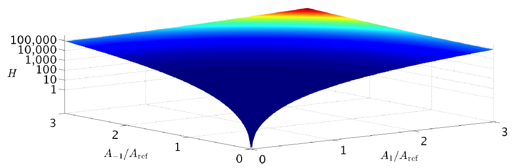
Figure 2: (Color online) Hamiltonian density of cw solutions of a BEC of ²³Na atoms in their ground state, having no particles with spin component $M_{F}=0$. The quantities are shown in dimensionless units [see Eq. (4c)], for generality and to avoid large amounts of notation. The cws in the figure have a fixed unit difference between the $M_{F}=1$ and $M_{F}=-1$ spin components wavenumbers, $k_{1}-k_{-1}=1$, and the magnetic field is zero. The Hamiltonian density is shown for a range of magnitudes of the BEC fields with $M_{F}=\pm 1$. The (dimensionless) reference amplitude on the axes is $A_{\mathrm{ref}}\equiv[\hbar^{2}(k_{1}-k_{-1})^{2}/8m+qB^{2}]/c_{2}$.

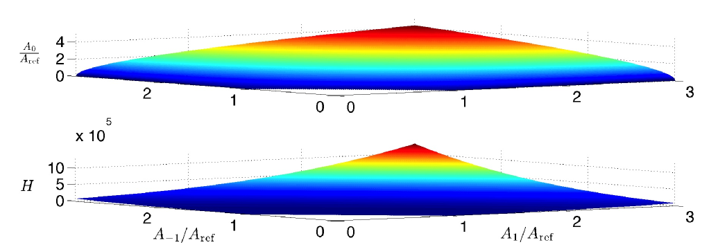
Figure 3: (Color online) Amplitude of the spin $M_{F}=0$ component and Hamiltonian density for cw solutions of a BEC of ²³Na BEC, with the relative phase in the spin $M_{F}=0$ component corresponding to even $n$ in the trial function (8), with $\theta_{1}+\theta_{-1}-2\theta_{0}=n\pi$. The quantities are shown in dimensionless units [see Eqs. (4c)]. The cws in the figure have a fixed unit difference between the $M_{F}=1$ and $M_{F}=-1$ spin components wavenumbers, $k_{1}-k_{-1}=1$, and the magnetic field is zero. The magnitude of the spin $M_{F}=0$ amplitude and the Hamiltonian density of the cw is shown for a range of magnitudes of the BEC fields with $M_{F}=\pm 1$. The (dimensionless) reference amplitude is $A_{\mathrm{ref}}\equiv[\hbar^{2}(k_{1}-k_{-1})^{2}/8m+qB^{2}]/c_{2}$.

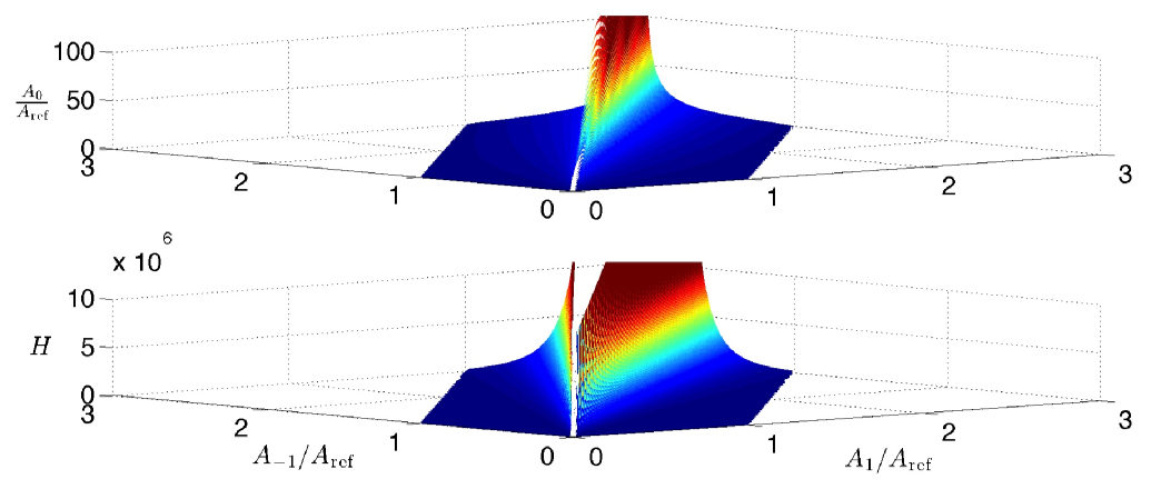
Figure 4: (Color online) Amplitude of the spin $M_{F}=0$ component and Hamiltonian density for cw solutions of a BEC of ²³Na BEC, with the relative phase in the spin $M_{F}=0$ component corresponding to odd $n$ in the trial function Eq. (8), with $\theta_{1}+\theta_{-1}-2\theta_{0}=n\pi$. The quantities are shown in dimensionless units [see Eq. (4c)]. The cws in the figure have a fixed unit difference between the $M_{F}=1$ and $M_{F}=-1$ spin components wavenumbers, $k_{1}-k_{-1}=1$, and the magnetic field is zero. The magnitude of the spin $M_{F}=0$ amplitude and the Hamiltonian density of the cw is shown for a range of magnitudes of the BEC fields with $M_{F}=\pm 1$. The (dimensionless) reference amplitude is $A_{\mathrm{ref}}\equiv[\hbar^{2}(k_{1}-k_{-1})^{2}/8m+qB^{2}]/c_{2}$. For odd $n$, the particle density of the $M_{F}=0$ BEC (as well as its Hamiltonian density) approaches infinity as the values of the densities of $M_{F}=1$ and $M_{F}=-1$ fields approach equality.

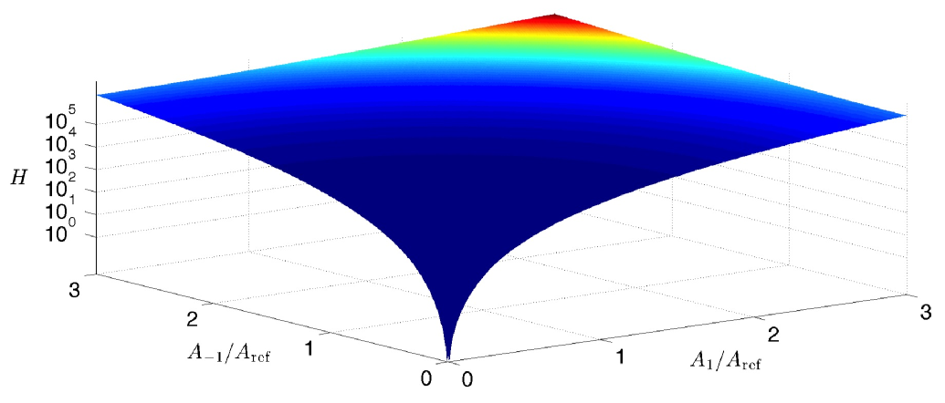
Figure 5: (Color online) Hamiltonian density of cw solutions of a BEC of ⁸⁷Rb atoms in their ground state, having no particles with spin component $M_{F}=0$. The quantities are shown in dimensionless units [see Eq. (4c)], for generality and to avoid large amounts of notation. The cws have a fixed unit difference between the $M_{F}=1$ and $M_{F}=-1$ spin components wavenumbers, $k_{1}-k_{-1}=1$, and the magnetic field is zero. The Hamiltonian density is shown for a range of magnitudes of the BEC fields with $M_{F}=\pm 1$. The (dimensionless) reference amplitude on the axes is $A_{\mathrm{ref}}\equiv-[\hbar^{2}(k_{1}-k_{-1})^{2}/8m+qB^{2}]/c_{2}$.

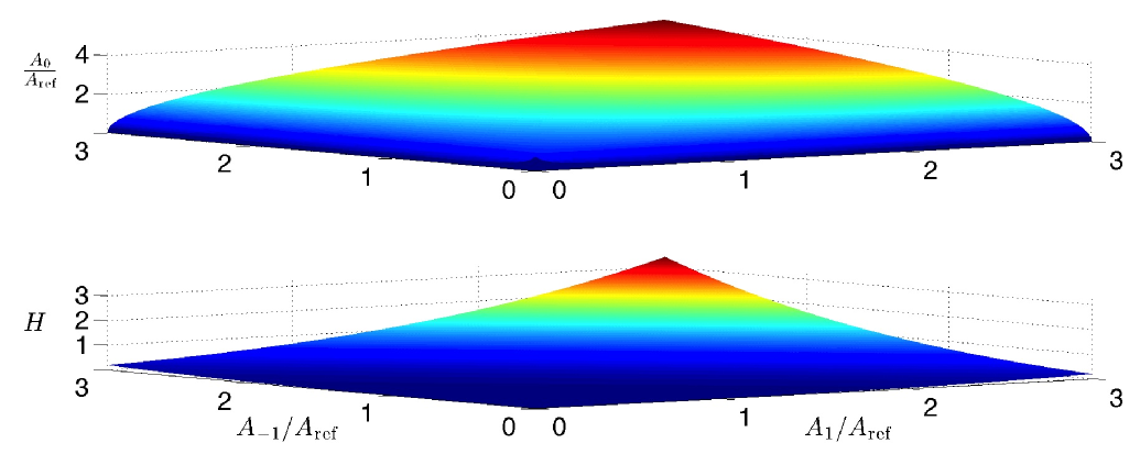
Figure 6: (Color online) Amplitude of the spin $M_{F}=0$ component and Hamiltonian density for cw solutions of a BEC of ⁸⁷Rb BEC, with the relative phase in the spin $M_{F}=0$ component corresponding to even $n$ in the trial function Eq. (8), with $\theta_{1}+\theta_{-1}-2\theta_{0}=n\pi$. The quantities are shown in dimensionless units [see Eq. (4c)]. These cws have a fixed unit difference between the $M_{F}=1$ and $M_{F}=-1$ spin components wavenumbers, $k_{1}-k_{-1}=1$, and the magnetic field is zero. The magnitude of the spin $M_{F}=0$ amplitude and the Hamiltonian density of the cw is shown for a range of magnitudes of the BEC fields with $M_{F}=\pm 1$. The (dimensionless) reference amplitude is $A_{\mathrm{ref}}\equiv-[\hbar^{2}(k_{1}-k_{-1})^{2}/8m+qB^{2}]/c_{2}$.

We carried out a stability analysis of the cw solutions within the continuous wave assumption, i.e., without looking for modulational (Benjamin-Feir) instabilities or sound waves (alias Bogoliubov excitations or phonons), that is, small perturbations of arbitrary wavenumber on top of the cw solutions Bogoliubov.1947 ; BespalovTalanov.1966 ; Andrews.1997 ; Andrews.1998 . A study of the sound waves and modulational stabilities is a large and lengthy topic. We will defer these results to another article. References Robins.2001 ; Konotop.2002 ; Li.2005 ; KawaguchiUeda.2012 analyze sound waves and modulational instabilities on top of subsets of the complete set of possible cw solutions herein. The stability analysis generalizes the ansatz (8) by allowing the variables for the magnitudes of the amplitudes $A_{1,0,-1}$, their phases $\theta_{1,0,-1}$, and wavenumbers $k_{1,0,-1}$ to vary with time. Inserting this ansatz into the dynamical equations (3) gives the results that the total particle density, $N\equiv A_{1}^{2}+A_{0}^{2}+A_{-1}^{2}$, and the magnetization, $M\equiv A_{1}^{2}-A_{-1}^{2}$, are conserved. Moreover, the wavenumbers $k_{1,0,-1}$ are do not change with time, due to the physics with the cw assumption. We may reduce the oscillations about the fixed points that represent the cw solutions to the dynamics of two variables, $A_{0}(t)^{2}$ and $[\theta_{1}(t)+\theta_{-1}(t)-2\theta_{0}(t)]$ which are conjugate to each other. The fixed points are stable to small perturbations, with frequencies

$$\omega_{n=0,1}^{2}=4\left(\frac{c_{2}}{\hbar}\right)^{2}A_{1}A_{0}^{2}A_{-1}\left[3(-1)^{n}+2\left(\frac{A_{1}}{A_{-1}}+\frac{A_{-1}}{A_{1}}\right)+\frac{(A_{1}^{2}-A_{-1}^{2})^{2}A_{0}^{2}}{4A_{1}^{3}A_{-1}^{3}}\right]\,.$$ (16)

The frequencies are always real-valued. Thus, all the $n=0,1$ cw solutions are stable within the continuous wave framework (i.e., not considering modulational instabilities, which due to length is deferred to another paper). Physically, these are the frequencies of oscillatory coherent spin mixing Zhang.2005 ; Gerbier.2006 ; MurPetit.2009 .

This oscillation is not the same as that in Refs. SzankowskiTrippenbachInfeldRowlands.2010 andSzankowskiTrippenbachInfeldRowlands.2011 . In those papers, the frame of reference can be rotated such that the solutions have no BEC component with spin $M_{F}=0$. The governing equations then reduce to two coupled nonlinear Schrödinger equations, without any parametric terms that either mix the spin components or lock their frequencies (chemical potentials) together. If such solutions are viewed in a rotated reference frame that mixes the spin components, there is an oscillation due to the beating of one frequency and wavenumber against another. The oscillations with frequencies (16), in contrast, cannot be eliminated by a change in the variables. There is just one oscillatory frequency for a given near-cw solution. One could rotate such a near-CW solution with a small oscillation into another reference frame, and get oscillations as in Refs. SzankowskiTrippenbachInfeldRowlands.2010 ; SzankowskiTrippenbachInfeldRowlands.2011 on top of the frequency (16) of the small variations about the fixed point. The oscillations in Refs. SzankowskiTrippenbachInfeldRowlands.2010 can be affected by linear Zeeman splitting; the oscillation frequencies (16) are independent of it.

IV Summary and Conclusions

We obtained the most general continuous wave (plane wave) solutions for spinor BECs for spin $F=1$, with linear and quadratic Zeeman splitting due to a magnetic field. We do not make the assumption that the wavenumbers of the different spin components are all the same. The physics only requires that cw solutions have wavenumbers and frequencies in the $M_{F}=0$ fields that are the average of the quantities in the $M_{F}=\pm 1$ fields. There are three distinct families of cw solutions. The first family are the solutions in which the $M_{F}=0$ spin component vanishes. The second and third families of cw solutions have non-zero densities of particles with spin $M_{F}=0$. The second and third families of solutions are distinguished from each other by the phase of the $M_{F}=0$ BEC field with respect to the average phase of the $M_{F}=\pm 1$ BEC fields. Other things being equal, the different phases in the $M_{F}=0$ fields give the cw solutions different densities of spin $M_{F}=0$ particles. The third family does not allow all the wavenumbers to be identical; in this limit, the density of $M_{F}=0$ particles is asymptotically large.

The first family of solutions, without spin $M_{F}=0$ particles, is governed by the coupled nonlinear Schrödinger equations, which have been studied in great detail. The solutions of the second and third type depend on whether the BEC is ferromagnetic or polar (antiferromagnetic). There are always cw solutions of the first type, and there is always at least one solution of the second or third type.

The linear Zeeman splitting term, with a constant uniform magnetic field, can be eliminated by a gauge transformation, so it does not change the dynamics. Quadratic Zeeman splitting cannot be eliminated, and has nontrivial effects. If the quadratic Zeeman coefficient is positive (which is the usual case for $F=1$ particles), it’s effects on the cw solutions are similar to the effects of a difference in the wavenumbers in the spin components. If the quadratic Zeeman coefficient is negative (which can be achieved by using microwaves and the Stark effect), a sufficiently large magnetic field can made the cw solutions in the $F=1$ spinor BEC switch from ferromagnetic to antiferromagnetic and vice versa.

The cw solutions of the second and third families are stable to small perturbations within the cw ansatz. We calculated the frequency of these perturbations, which correspond to oscillatory coherent spin mixing.

- (1) D. G. Fried, T. C. Killian, L. Willmann, D. Landhuis, S. C. Moss, D. Kleppner, and T. J. Greytak, “Bose-Einstein Condensation of Atomic Hydrogen,” Phys. Rev. Lett. 81, 3811-3814 (1998).
- (2) C. C. Bradley, C. A. Sackett, J. J. Tollett, and R. G. Hulet , “Evidence of Bose-Einstein Condensation in an Atomic Gas with Attractive Interactions,” Phys. Rev. Lett. 75, 1687-1690 (1995).
- (3) C. C. Bradley, C. A. Sackett, and R. G. Hulet, “Bose-Einstein Condensation of Lithium: Observation of Limited Condensate Number,” Phys. Rev. Lett. 78, 985-989 (1997).
- (4) M. V. Simkin and E. G. D. Cohen, “Magnetic properties of a Bose-Einstein condensate,” Phys. Rev. A 59, 1528-1532 (1999).
- (5) G. Roati, M. Zaccanti, C. D’Errico, J. Catani, M. Modugno, A. Simoni, M. Inguscio, and G. Modugno, “39K Bose-Einstein Condensate with Tunable Interactions,” Phys. Rev. Lett. 99, 010403 (2007).
- (6) G. Modugno, G. Ferrari, G. Roati, R. J. Brecha, A. Simoni, and M. Inguscio, “Bose-Einstein Condensation of Potassium Atoms by Sympathetic Cooling,” Science 294, 1320-1322 (2001).
- (7) A. Griesmaier, J. Werner, S. Hensler, J. Stuhler, and T. Pfau, “Bose-Einstein Condensation of Chromium,” Phys. Rev. Lett. 94, 160401 (2005).
- (8) Q. Beaufils, R. Chicireanu, T. Zanon, B. Laburthe-Tolra, E. Marechal, L. Vernac, J.-C. Keller, and O. Gorceix, “All-optical production of chromium Bose-Einstein condensates,” Phys. Rev. A 77, 061601(R) (2008).
- (9) M. D. Barrett, J. A. Sauer, and M. S. Chapman, “All-Optical Formation of an Atomic Bose-Einstein Condensate,” Phys. Rev. Lett. 87, 010404 (2001).
- (10) M.-S. Chang, C. D. Hamley, M. D. Barrett, J. A. Sauer, K. M. Fortier, W. Zhang, L. You, and M. S. Chapman, “Observation of Spinor Dynamics in Optically Trapped 87Rb Bose-Einstein Condensates,” Phys. Rev. Lett. 92, 140403 (2004).
- (11) L. E. Sadler, J. M. Higbie, S. R. Leslie, M. Vengalattore, and D. M. Stamper-Kurn, “Spontaneous symmetry breaking in a quenched ferromagnetic spinor Bose-Einstein condensate,” Nature (London) 443, 312-315 (2006).
- (12) S. R. Leslie, J. Guzman, M. Vengalattore, J. D. Sau, M. L. Cohen, and D. M. Stamper-Kurn, “Amplification of fluctuations in a spinor Bose-Einstein condensate,” Phys. Rev. A 79, 043631 (2009).
- (13) T. Weber, J. Herbig, M. Mark, H.-C. Nagerl, and R. Grimm, “Bose-Einstein Condensation of Cesium,” Science 299, 232-235 (2003).
- (14) M. Lu, N. Q. Burdick, S. H. Youn, and B. L. Lev, “Strongly Dipolar Bose-Einstein Condensate of Dysporium,” Phys. Rev. Lett. 107, 190401 (2011).
- (15) K. Aikawa, A. Frisch, M. Mark, S. Baier, A. Rietzler, R. Grimm, and F. Ferlaino, “Bose-Einstein Condensation of Erbium,” Phys. Rev. Lett. 108, 210401 (2012).
- (16) S. Gupta, K. W. Murch, K. L. Moore, T. P. Purdy, and D. M. Stamper-Kurn, “Bose-Einstein Condensation in a Circular Waveguide,” Phys. Rev. Lett. 95, 143201 (2005).
- (17) S. E. Olson, M. L. Terraciano, M. Bashkansky, and F. K. Fatemi, “Cold-atom confinement in an all-optical dark ring trap,” Phys. Rev. A 76, 061404(R) (2007).
- (18) I. Lesanovsky and W. von Klitzing, “Time-Averaged Adiabatic Potentials: Versatile Matter-Wave Guides and Atom Traps,” Phys. Rev. Lett. 99, 083001 (2007).
- (19) K. Henderson, C. Ryu, C. MacCormick, and M. G. Boshier, “Experimental demonstration of painting arbitrary and dynamic potentials for Bose-Einstein condensates,” New J. Phys. 11, 043030 (2009).
- (20) C. Ryu, M. F. Andersen, P. Clade, V. Natarajan, K. Helmerson, and W. D. Phillips, “Observation of Persistent Flow of a Bose-Einstein Condensate in a Toroidal Trap,” Phys. Rev. Lett. 99, 260401 (2007).
- (21) M. Ueda, “Bose Gases with Nonzero Spin,” Ann. Rev. Condens. Matter Phys. 3, 263-283 (2012).
- (22) Y. Kawaguchi and M. Ueda, “Spinor Bose-Einsetin Condensates,” Physics Reports 520, 253-381 (2012).
- (23) H. Saito, Y. Kawaguchi, and M. Ueda, “Topological defect formation in a quenched ferromagnetic Bose-Einstein condensates,” Phys. Rev. A 75, 013621 (2007).
- (24) A. Lamacraft, “Quantum Quenches in a Spinor Condensate,” Phys. Rev. Lett. 98, 160404 (2007).
- (25) W. Zhang, D. L. Zhou, M.-S. Chang, M. S. Chapman, and L. You, “Coherent spin mixing dynamics in a spin-1 atomic condensate,” Phys. Rev. A 72, 013602 (2005).
- (26) F. Gerbier, A. Widera, S. Fölling, O. Mandel, and I. Bloch, “Resonant control of spin dynamics in ultracold quantum gases by microwave dressing,” Phys. Rev. A 73, 041602(R) (2006).
- (27) N. P. Robins, W. Zhang, E. A. Ostrovskaya, and Y. S. Kivshar, “Modulational instability of spinor condensates,” Phys. Rev. A 64, 021601(R) (2001).
- (28) V. V. Konotop and M. Salerno, “Modulational instability in Bose-Einstein condensates in optical lattices,” Phys. Rev. A 65, 021602(R) (2002).
- (29) L. Li, Z. Li, B. A. Malomed, D. Mihalache, and W. M. Liu, “Exact soliton solutions and nonlinear modulation instability in spinor Bose-Einstein condensates,” Phys. Rev. A 72, 033611 (2005).
- (30) J. Ieda, T. Miyakawa, and M. Wadati, “Exact Analysis of Soliton Dynamics in Spinor Bose-Einstein Condensates,” Phys. Rev. Lett. 93, 194102 (2004).
- (31) M. Wadati and N. Tsuchida, “Wave Propagations in the F=1 Spinor Bose-Einstein Condensates,” J. Phys. Soc. Jpn. 75, 014301 (2006).
- (32) M. Uchiyama, J. Ieda, and M. Wadati, “Dark solitons in F=1 spinor Bose-Einstein condensate,” J. Phys. Soc. Jpn. 75, 064002 (2006).
- (33) J. Mur-Petit, “Spin dynamics and structure formation in a spin-1 condensate in a magnetic field,” Phys. Rev. A 79, 063603 (2009)
- (34) P. Szankowski, M. Trippenbach, and E. Infeld, and G. Rowlands, “Oscillating Solitons in a Three-Component Bose-Einstein Condensate,” Phys. Rev. Lett 105, 125302 (2010).
- (35) P. Szankowski, M. Trippenbach, E. Infeld, and G. Rowlands, “Class of compact entities in three-component Bose-Einstein condensates,” Phys. Rev. A 83, 013626 (2011).
- (36) T. Ohmi and K. Machida, “Bose-Einstein Condensation with Internal Degrees of Freedom in Alkali Atom Gases,” J. Phys. Soc. Jpn. 67, 1822-1825 (1998).
- (37) T. -L. Ho, “Spinor Bose Condensates in Optical Traps,” Phys. Rev. Lett. 81, 742-745 (1998).
- (38) M. Olshanii, “Atomic Scattering in the Presence of an External Confinement and a Gas of Impenetrable Bosons,” Phys. Rev. Lett. 81, 938 (1998).
- (39) T. Bergeman, M. G. Moore, and M. Olshanii, “Atom-Atom Scattering under Cylindrical Harmonic Confinement: Numerical and Analytic Studies of the Confinement Induced Resonance,” Phys. Rev. Lett. 91, 163201 (2003).
- (40) M.-S. Chang, Q. Qin, W. Zhang, L. You, and M. S. Chapman, “Coherent spinor dynamics in a spin-1 Bose condensate,” Nature Phys. 1, 111-116 (2005).
- (41) N. N. Klausen, J. L. Bohn, and C. H. Greene, “Nature of spinor Bose-Einstein condensates in rubidium,” Phys. Rev. A 64, 053602 (2001).
- (42) E. G. M. van Kempen, S. J. J. M. F. Kokkelmans, D. J. Heinzen, and B. J. Verhaar, “Interisotope Determination of Ultracold Rubidium Interactions from Three High-Precision Experiments,” Phys. Rev. Lett. 88, 093201 (2002).
- (43) S. V. Manakov, “On the theory of two-dimensional stationary self-focusing of electromagnetic waves,” Zh. Eksp. Teor. Fiz. 65, 505-516 (1973) [Sov. Phys.-JETP 38, 248-253 (1974)].
- (44) K. Nakkeeran, K. Porsezian, P. S. Sundaram, and A. Mahalingam, “Optical Solitons in N-Coupled Higher Order Nonlinear Schrödinger Equations,” Phys. Rev. Lett. 80, 1425-1428 (1998).
- (45) J. Ieda and M. Wadati, “Nonlinear Dynamics of Spin Structure in Confined Bose-Einstein Condensates,” J. Low Temp. Phys. 148, 405-410 (2007).
- (46) V. E. Zakharov and A. B. Shabat, “Exact Theory of Two-dimensional Self-focusing and One-dimensional Self-modulation of Waves in Nonlinear Media,” Zh. Eksp. Teor. Fiz. 61, 118-134 (1971) [Sov. Phys. JETP 34, 62-69 (1972)].
- (47) V. E. Zakharov and A. B. Shabat, “Interaction between solitons in a stable medium,” Zh. Eksp. Teor. Fiz. 64, 1627-1639 (1973) [Sov. Phys. JETP 37, 823-828 (1973)].
- (48) J. Yang, Nonlinear Waves in Integrable and Nonintegrable Systems (SIAM, Philadelphia, 2010).
- (49) V. E. Zakharov and E. I. Schulman, “To the integrability of the system of two coupled nonlinear Schrödinger equations,” Physica D 4, 270-274 (1982).
- (50) G. P. Agrawal, Applications of Nonlinear Fiber Optics (Academic, NY, 2001).
- (51) Y. S. Kivshar and S. K. Turitsyn “Vector dark solitons,” Opt. Lett. 18, 337-339 (1993).
- (52) R. Radhakrishnan and M. Lakshmanan, “Bright and dark soliton solutions to coupled nonlinear Schrödinger equations,” J. Phys. A: Math. Gen. 28, 2683-2692 (1995).
- (53) R. Radhakrishnan, M. Lakshmanan, and M. Daniel, “Bright and dark optical solitons in coupled higher-order nonIinear Schrödinger equations through singularity structure analysis,” J. Phys. A Math. Gen. 28, 7299-7314 (1995).
- (54) M. Haelterman and A. P. Sheppard, “Bifurcations of the dark soliton and polarization domain walls in nonlinear dispersive media,” Phys. Rev. E 49, 4512-4518 (1994).
- (55) B. A. Malomed, “Domain wall between traveling waves,” Phys. Rev. E 50, R3310-R3313 (1994).
- (56) N. N. Bogoliubov, “On the Theory of Superfluidity,” Izv. Akad. Nauk. SSSR Ser. Fiz. 11, 77-90 (1947) [J. Phys. (Moscow) 11, 23-32 (1947)].
- (57) V. I. Bespalov and V. I. Talanov, “Filamentary Structure of Light Beams in Nonlinear Media,” Pis’ma Zh. Eksp. Teor. Fiz. 3, 471-476 (1966) [JETP Lett. 3, 307-310 (1966)].
- (58) M. R. Andrews, D. M. Kurn, H.-J. Miesner, D. S. Durfee, C. G. Townsend, S. Inouye, and W. Ketterle, “Propagation of Sound in a Bose-Einstein Condensate,” Phys. Rev. Lett. 79, 553-556 (1997).
- (59) M. R. Andrews, D. M. Stamper-Kurn, H.-J. Miesner, D. S. Durfee, C. G. Townsend, S. Inouye, and W. Ketterle, “Erratum: Propagation of Sound in a Bose-Einstein Condensate,” Phys. Rev. Lett. 80, 2967 (1998).