Roche volume filling of star clusters in the Milky Way

Abstract

We examine the ratios $r_{h}/r_{J}$ of projected half-mass and Jacobi radius as well as $r_{t}/r_{J}$ of tidal and Jacobi radius for open and globular clusters in the Milky Way using data of both observations and simulations. We applied an improved calculation of $r_{J}$ for eccentric orbits of globular clusters. A sample of 236 open clusters of Piskunov et al. within the nearest kiloparsec around the Sun has been used. For the Milky Way globular clusters, data are taken from the Harris catalogue. We particularly use the subsample of 38 Milky Way globular clusters for which orbits have been integrated by Dinescu et al. We aim to quantify the differences between open and globular clusters and to understand, why they form two intrinsically distinct populations. We find under certain assumptions, or, in other words, in certain approximations, (i) that globular clusters are presently Roche volume underfilling and (ii) with at least $3\sigma$ confidence that the ratio $r_{h}/r_{J}$ of half-mass and Jacobi radius is $3-5$ times larger at present for an average open cluster in our sample than for an average globular cluster in our sample and (iii) that a significant fraction of globular clusters may be Roche volume overfilling at pericentre with $r_{t}>r_{J}$. Another aim of this paper is to throw light on the underlying theoretical reason for the existence of the van den Bergh correlation between half-mass and galactocentric radius.

1 Introduction

Open star clusters (OCs) are abundant in the Milky Way disc. Their number is estimated to be of order $10^{5}$ (Piskunov et al., 2006). In contrast, there are approximately 150 globular clusters (GCs) known in the Milky Way (Harris, 1996, 2010 edition). While the GCs are orbiting on eccentric orbits with partly high inclinations with respect to the stellar disc plane of the Milky Way, most OCs reside on near-circular orbits in the disc (although they may show a vertical oscillation with an amplitude of order $\approx 0.5$ kpc (Cararro & Chiosi, 1994). The GCs are long-lived with a mean age of 10 Gyr. The OCs are short-lived with a mean lifetime of only 300 Myr (Binney & Tremaine, 2008, Figure 8.5, hereafter: BT2008). Moreover, the lifetimes of OCs range from a few tens of Myr to a few Gyr. Age distributions are also given by Lamers & Gieles (2006) and Bonatto & Bica (2011).

Baumgardt et al. (2010) presented a weak evidence that there are two distinct GC populations outside the solar radius, namely a population of massive compact clusters with very small half-mass radii compared to the Jacobi radius and a population of low-mass and extended clusters with $r_{h}/r_{J}>0.1$. They argued that King models allow only a restricted range of $r_{\mathrm{h}}/r_{\mathrm{t}}$ and used the half-mass radius to quantify the Roche volume filling of GCs. However, there are other dynamical models like polytropes (see, e.g., Converse & Stahler, 2010) with a much larger half mass radius compared to the tidal radius. Additionally Baumgardt et al. used the Jacobi radius of circular orbits instead of the more general definition provided by King (1962) for eccentric orbits (see Appendix B4 for a more detailed comparison to the present work). We apply a more general derivation for circular and eccentric orbits including $r_{\mathrm{h}}$ and $r_{\mathrm{t}}$ in order to distinguish the compactness of a cluster and the Roche volume filling factor.

It has been shown by van den Bergh (1994), that the half-light radii $r_{h}$ of GCs are correlated with the Galactocentric radius $R$ according to the relation

$$r_{h}\propto R^{2/3}$$ (1)

This relation has never been explained in terms of a deeper physical reason, although van den Bergh suspected already in 1994 that the correlation (1) could be imposed by the underlying galactic tidal field. Assuming that the GCs are moving in an isothermal halo we find from analytical calculations that the time-dependent Jacobi radius (i.e., the distance to the Lagrange points $L_{1}$ and $L_{2}$) for eccentric orbits in such a halo scales as

$$\lim_{R\gg L/V_{C}}r_{J,\,\rm isoth.}\propto R^{2/3}$$ (2)

(see appendix B.2). From the assumption of an isothermal halo, Eqns. (1) and (2) and $\langle R\rangle\gg\langle L\rangle/V_{C}$, where $\langle R\rangle,\langle L\rangle$ and $V_{C}$ are median Galactocentric radius, orbital angular momentum and the halo’s circular velocity, respectively, it is possible to conclude that GCs in the Milky Way are characterized by a ratio $r_{h}/r_{J}$ which is independent of $R$. The consequence is that, within the scatter of the correlation (which may be due to the scatter in GC masses), GCs are characterized by a common average relative size. We note that the Jacobi radius (i.e., the distance from the cluster centre to the Lagrange points $L_{1}$ and $L_{2}$) provides a natural scale for star clusters in the tidal field. Other (dependent) scales are given by the positions/widths of the dominant resonances in the star cluster.

To gain a better understanding of the difference between OCs and GCs and why they form two distinct populations, one may ask: Which values takes ratio $r_{h}/r_{J}$ on in the case of OCs. While for GCs on eccentric orbits we may assume that their size is enforced by quantities in the pericenter, it seems reasonable to suspect that OCs on near-circular orbits are not strongly influenced by the orbital evolution.

In the following discussions, we denote the ratio $r_{h}/r_{J}$ of 3D half-mass radius and Jacobi radius with the letter $\lambda$. We also define $\widehat{\lambda}=r_{t}/r_{J}$ using the cluster cutoff radii $r_{t}$ (i.e. the radii at which the density drops to zero) instead of the projected half-mass radii $r_{h}$.

The 3D half-mass radius $r_{h}=r_{h,\rm 3D}$ of a spherically symmetric stellar system is typically larger than the projected (2D) half-mass radius $r_{h,\rm 2D}$. We have $r_{h,\rm 3D}\approx 1.3\,r_{h,\rm 2D}$. For the Plummer model $r_{h,\rm 3D}/r_{h,\rm 2D}\approx 1.30$ can be obtained analytically.

This paper is organized as follows: Section 2 presents the theory, section 3 lists the current status of observations and simulations. In Section 4 the results are calculated and Section 5 contains the discussion and conclusions.

2 Theory

Following the approach by King (1962), the Jacobi radius of a star cluster in the tidal field of a galaxy (i.e. the distance from the star cluster center to the Lagrange points $L_{1}$ and $L_{2}$) can generally be written as

$$r_{J}=\left[\frac{GM_{cl}}{\Omega^{2}-\frac{d^{2}\Phi}{dR^{2}}}\right]^{1/3}$$ (3)

where $G$, $M_{\rm cl}$, $\Omega$, $\Phi$ and $R$ are the gravitational constant, the star cluster mass, the angular speed, the gravitational potential of the galaxy and the galactocentric radius, respectively. The last closed (critical) equipotential surface through the Lagrange points $L_{1}$ and $L_{2}$ encloses the Roche or Hill volume.

Furthermore we define the “(circular) velocity radius”

$$r_{v}=\frac{GM_{cl}}{V_{\rm C}^{2}}$$ (4)

It is the length scale at which the Keplerian circular velocity in the cluster (assuming a point mass cluster potential) would be equal to the circular velocity $V_{\rm C}$ in the Milky Way.

The orbital periods $t_{\rm orb}$ and $T_{\rm orb}$ of a star at the half-mass radius of the star cluster and that of the star cluster orbit around the galaxy, respectively, are given by

$$t_{\rm orb} = \pi t_{\rm cr}=\frac{2\pi r_{h}}{\sigma_{0}}\approx 2\pi\sqrt{\frac{2r_{h}^{3}}{GM_{\rm cl}}}\ \ \ \mathrm{and}$$ (5)

$$T_{\rm orb} = \frac{2\pi}{\Omega_{C}}=\frac{2\pi R_{C}}{V_{C}},$$ (6)

where $t_{\rm cr}$ is the crossing time (i.e. the time needed for a star to cross the half-mass sphere) and $\sigma_{0}^{2}\approx GM_{\rm cl}/(2r_{h})$ in dynamical equilibrium.

2.1 Circular orbits

For an OC on a circular orbit with radius $R_{\rm C}$ and velocity $V_{C}$ in a tidal field the Jacobi radius from Eqn. (3) can be written as (King, 1962; Küpper et al., 2008; Just et al., 2009)

$$r_{J}=\left[\frac{GM_{\rm cl}}{(4-\beta_{C}^{2})\Omega_{C}^{2}}\right]^{1/3}=\left(4-\beta_{C}^{2}\right)^{-1/3}r_{v}^{1/3}R_{\rm C}^{2/3}$$ (7)

with $\beta_{C}=\kappa_{C}/\Omega_{C}$ (see appendix A), where $G$, $M_{\rm cl}$, $\kappa_{C}$, $\Omega_{C}$ and $R_{C}$ are the gravitational constant, the total mass of the star cluster, the epicyclic and the circular frequency and the obital radius, respectively, and $r_{v}$ is given by Eqn. (4).

Inserting (5) and (6) into (7) yields

$$\lambda_{\rm OC}=\left(\frac{r_{h}}{r_{J}}\right)_{\rm OC}=\left(\frac{4-\beta_{C}^{2}}{2}\right)^{1/3}\left(\frac{t_{\rm orb}}{T_{\rm orb}}\right)_{\rm OC}^{2/3}$$ (8)

for star clusters on circular orbits.

While $r_{J}$ determines the geometry of equipotential surfaces and cannot be observed, $r_{h}$, $t_{\rm cr}\propto r_{h}/\sigma_{0}$ and $T_{\rm orb}$ can be determined by observations and simulations. For realistic Milky Way models, the ratio $\beta_{C}$ is approximately constant as a function of Galactocentric radius and the dependency on it is so weak (see Figure 1 and appendix A) that we can safely neglect its variation beyond $2-3$ kpc of the center of the Milky Way.

2.2 Eccentric orbits

For GCs on eccentric orbits in an isothermal halo ($V_{C}=\mathrm{const}$) we must extend the theory (see appendix B.2). Following the approach by King (1962) the Jacobi radius from Eqn. (3) can be written as

$$r_{J}=r_{v}^{1/3}\left(\frac{R^{4}}{R_{g}^{2}+R^{2}}\right)^{1/3}$$ (9)

where $R=R(t)$ is time-dependent, $r_{v}$ is given by Eqn. (4), $V_{C}$ is the rotation speed of the isothermal sphere, $R_{g}=L/V_{C}$ is a guiding radius and the angular momentum $L=L(V_{C},R_{P},R_{A})$ is a constant of motion given by Eqn. (36). From Eqns. (3) and (5) we also find

$$\lambda_{\rm GC} = \left(\frac{r_{h}}{r_{J}}\right)_{\rm GC}=\left(\frac{t_{\rm orb}}{2\pi}\right)^{2/3}\left[\frac{L^{2}}{R(t)^{4}}+\frac{V_{C}^{2}}{R(t)^{2}}\right]^{1/3}$$ (10)

$$= \left(\frac{t_{\rm orb}}{2\pi}\right)^{2/3}\left(\frac{V_{C}^{2}}{2}\right)^{1/3}\left(\frac{R_{g}^{2}+R(t)^{2}}{R(t)^{4}}\right)^{1/3}.$$ (11)

We distinguish between two cases:

1. With the van-den-Bergh correlation (1) we obtain from Eqn. (5) along one orbit

   $$t_{\rm orb}\propto R$$ (12)

   and

   $$\frac{t_{\rm orb}(t)}{R(t)}=\frac{t_{\rm orb,P}}{R_{P}}=\frac{t_{\rm orb,A}}{R_{A}},\ \ \ \ \ \frac{t_{\rm orb}}{T_{\rm orb}}=\mathrm{const}$$ (13)

   where the subscripts “P” and “A” stand for peri- and apocenter. From Eqn. (10) we obtain with (12)

   $$\lambda_{\rm GC}^{3}\propto\frac{A}{R^{2}}+B$$ (14)

   where $A$ and $B$ are two constants. It follows that

   $$\lim_{R\gg R_{g}}\lambda_{\rm GC}=\mathrm{const},\ \ \ \ \ \lim_{R\ll R_{g}}\lambda_{\rm GC}\propto R^{-2}$$ (15)

   where $R_{g}$ is given by Eqn. (41).

2. Contrariwise, direct $N$-body simulations suggest that for a bound GC the half-mass radius changes more slowly than the time scale $T_{\rm orb}$ while the Jacobi radius oscillates on that time scale according to Eqn. (40) (see Figure 2). This would mean that, if $M_{cl}\approx\mathrm{const}$,

   $$t_{\rm orb}\approx\mathrm{const}$$ (16)

   in difference to Eqn. (12). From Eqn. (10) we obtain with (16)

   $$\lambda_{\rm GC}^{3}\propto\frac{C}{R^{4}}+\frac{D}{R^{2}}$$ (17)

   where $C$ and $D$ are two constants.

Figure 1: The ratio $\beta_{C}$ at $z=0$ for the JSH95 and P90 models of Dinescu et al. (1999) and the three-component Plummer-Kuzmin (3PLK) model used in Kharchenko et al. (2009) and Just et al. (2009).

Figure 2: Time evolution of half-mass and Jacobi radii for a direct $N$-body simulation of a star cluster with $N=50000$ particles on an eccentric orbit within the disc plane. The cluster has a standard double-segment Kroupa (2001) IMF and is initially Roche volume filling, i.e. the cutoff radius equals the Jacobi radius. The half-mass radius is calculated with respect to the current mass within the initial Jacobi radius. Both radii are scaled with the initial half-mass radius $r_{h,i}\approx 9$ pc.

3 Observations and simulations

3.1 Samples and medians for OCs and GCs

Table 1: Values for OCs and GCs. The values are medians if not denoted otherwise. The errors are standard errors of the median, i.e. divided by $\sqrt{N}$ of the sample size except for the error $\Delta T_{\rm orb,OC}$. The data for OCs are derived from Piskunov et al. (2007) and BT2008. The data for GCs are derived from Harris (1996, 2010 edition) and Dinescu et al. (1999).

OC parameter	Value
Sample size $N_{\rm OCs}$	236
Median projected half-mass radius $r_{h,\rm 2D}$ [pc]	$1.94\pm 0.15$
Median tidal radius $r_{t}$ [pc]	$7.90\pm 0.51$
Velocity dispersion $\sigma_{0}$ [pc Myr-1]	$0.31$
Median crossing time $t_{\rm cr,OC}=2r_{h,\rm 2D}/\sigma_{0}$ [Myr]	$12.52\pm 0.96$
Average orbital period $T_{\rm orb,OC}$ [Myr]	$220\pm 30$
Average eccentricity $e_{\rm OC}$	$0.127\pm 0.003$
GC parameter	Value
Sample size $N_{\rm GCs}$	34 (38)
Median half-light radius $r_{h,\rm 2D}$ [pc]	$3.13\pm 0.51$
Median tidal radius $r_{t}$ [pc]	$33.02\pm 4.83$
Median velocity disp. $\sigma_{0}$ [pc Myr-1]	$5.11\pm 0.64$
Median crossing time $t_{\rm cr,GC}=2r_{h,\rm 2D}/\sigma_{0}$ [Myr]	$1.175\pm 0.726$
Median Galactocentric radius $R_{\rm orb,GC}$ [kpc]	$7.75\pm 0.84$
Median height above the disc plane $z_{\rm GC}$ [kpc]	$4.00$
Median velocity $V_{\rm GC}$ [pc Myr-1]	$175\pm 16$
Median orbital period $T_{\rm orb,GC}$ [Myr]	$207\pm 54$
Median eccentricity $e_{\rm GC}$	$0.622\pm 0.044$

For OCs we use the sample of 236 OCs of Piskunov et al. (2007). We obtain the values given in the upper part of Table 1. The projected half-mass radii of the 236 OCs have been obtained by solving 236 transcendental equations with the Newton-Raphson method using the table of core and tidal radii provided by Piskunov et al. (2007) at the CDS. The transcendental equation is given by

$$\ln X_{h}+\frac{X_{h}}{C}-4\sqrt{\frac{X_{h}}{C}}-\frac{\ln C}{2}-\frac{1}{2C}-\frac{2}{\sqrt{C}}+\frac{3}{2}=0$$ (18)

with

$$X_{h}=1+(r_{h}/r_{c})^{2}\ \ \ \mathrm{and}\ \ \ C=1+(r_{t}/r_{c})^{2}$$ (19)

where $r_{c},r_{h}$ and $r_{t}$ are the core, half-mass and tidal cutoff radii, respectively (cf. Ernst et al., 2010, Section 3). Eqn. (18) is solved for $r_{h}$.

The error of the median value of the projected half-mass radius $r_{h,\rm 2D}$ is defined as

$$\Delta r_{h,\rm 2D}=\sqrt{\frac{\sum_{i=1}^{N_{\rm OCs}}\left[r_{h,i,\rm 2D}-\mathrm{Median}(r_{h,i,\rm 2D})\right]^{2}}{N_{\rm OCs}(N_{\rm OCs}-1)}}$$ (20)

We do not have an error on the velocity dispersion $\sigma_{0}$ of OCs. Thus we have set $\Delta\sigma_{0}=0$ for OCs. Note also that in a bound system $r_{h}$ and $\sigma_{0}$ are related through the virial theorem, i.e. we have $\Delta\sigma_{0}/\sigma_{0}=(1/2)\Delta r_{h}/r_{h}$ in virial equilibrium. We neglect this correlation since the virial theorem is not generally valid for star clusters in a tidal field. Namely, it is not valid for Roche volume overfilling star clusters. The derived crossing time and its relative error are given by

$$t_{\rm cr}=2r_{h,\rm 2D}/\sigma_{0},\ \ \ \Delta t_{\rm cr}/t_{\rm cr}=\sqrt{\left(\Delta r_{h}/r_{h}\right)^{2}+\left(\Delta\sigma_{0}/\sigma_{0}\right)^{2}}$$ (21)

The OCs in the sample by Piskunov et al. (2007) have approximately the orbital period of the Local Standard of Rest (LSR) taken from BT2008, table 1.2.

For GCs we use the median values from 34 out of a sample of 38 Milky Way globular clusters from Dinescu et al. (1999). The data compilation of 157 Milky Way GCs by Harris (Harris (1996, 2010 edition)) was also used. The median values are obtained from the equivalents of Eqns. (20) and (21) for the observed/simulated and the derived quantities. We obtained the values given in the bottom part of Table 1. Only for 97 out of 157 GCs from the Harris catalogue $\sigma_{0}$ is given. For 5 of these 97 GCs $r_{h}$ is not given as well. From the GC sample in Dinescu et al. (1999) with 38 GCs we further find a median value of the orbital period of GCs. Only for 34 out of 38 GCs in the Dinescu et al. sample $\sigma_{0}$ is given in the Harris catalogue. The minimum Galactocentric radius is $R=2.7$ kpc for NGC 6144 such that we can neglect the dependency on $\beta_{C}$ according to Figure 1. We further remark that a few recently discovered GCs have been added to Harris’ compilation by Ortolani et al. (2012).

4 Results

4.1 OCs

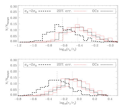
Figure 3: The ratios $r_{h,\rm 3D}/r_{J}$ (top panel) and $r_{t}/r_{J}$ (bottom panel) for OCs calculated from Eqn. (8) for the sample of Piskunov et al. (2007). The histograms for a canonical $\pm 20$% error on $\sigma_{0}$ and for the substitution $\sigma_{0}\rightarrow 2\sigma_{0}$ in Eqn. (8) are also shown. The vertical lines denote the medians. Note that $r_{h,\rm 2D}$ of the data set is corrected with a factor 1.3 to obtain $r_{h,\rm 3D}$.

Table 2: Quantiles for OCs.

Parameter	$10^{Q_{10}}$	$10^{Q_{50}}$	$10^{Q_{90}}$
$\lambda_{\rm OC}$, Table 1	0.239	0.379	0.675
$\lambda_{\rm OC}$, $\sigma_{0}\rightarrow 2\sigma_{0}$	0.151	0.239	0.425
$\widehat{\lambda}_{\rm OC}$, Table 1	0.506	0.812	1.35
$\widehat{\lambda}_{\rm OC}$, $\sigma_{0}\rightarrow 2\sigma_{0}$	0.319	0.511	0.852

Figure 3 shows the distributions of $\log_{10}\lambda_{\rm OC}$ (top panel) and $\log_{10}\widehat{\lambda}_{\rm OC}$ (bottom panel) for OCs according to Eqn. (8). We used the isothermal approximation $\beta_{C}=\sqrt{2}$. There is a large scatter of the sizes around the medians. We find also Roche volume overfilling OCs.

$\widehat{\lambda}_{\rm OC}$ was found from Eq. (8) with the values of Table 1 using the tidal radii instead of the half-mass radii in the definitions of crossing time (i.e, $t^{\prime}_{\rm cr}=2r_{t}/\sigma_{0}$ instead of $t_{\rm cr}=2r_{h}/\sigma_{0}$).

Figure 3 shows also the distributions of $\log_{10}\lambda_{\rm OC}$ with the substitution $\sigma_{0}\rightarrow 2\sigma_{0}$ which leads to $t_{\rm cr,OCs}\rightarrow t_{\rm cr,OCs}/2$ in Eqn. (10).

We find the medians $Q_{50}$ given in Table 2. The quantiles $Q_{10},Q_{50}$ and $Q_{90}$ have been calculated with an idl routine by Hong (Hong et al., 2004).

4.2 GCs

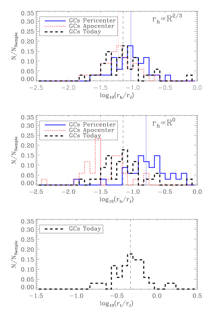
Figure 4: Top panel: The ratio $r_{h,\rm 3D}/r_{J}$ of GCs today and in the peri- and apocenter calculated from Eqn. (10) for 34 GCs out of the sample by Dinescu et al. (1999) under the assumption that the GCs are moving in an isothermal halo with $V_{C}\approx 228.5$ km/s and that the van-den-Bergh correlation holds. Middle panel: The same as in the top panel assuming that instead of the van-den-Bergh correlation $r_{h}$ is independent of Galactocentric radius. Bottom panel: The ratio $r_{t}/r_{J}$ for GCs today calculated from Eqn. (40). The vertical lines denote the medians. Note that $r_{h,\rm 2D}$ of the data set is corrected with a factor 1.3 to obtain $r_{h,\rm 3D}$.

Table 3: Quantiles for GCs. The subscript “0” denotes present-day values.

Parameter		$10^{Q_{10}}$	$10^{Q_{50}}$	$10^{Q_{90}}$
$\lambda_{\rm GC,0}$		0.0318	0.0701	0.239
$\widehat{\lambda}_{\rm GC,0}$		0.286	0.469	0.742
$\lambda_{\rm GC,P}$	($r_{h}\propto R^{2/3}$)	0.0427	0.0928	0.178
$\lambda_{\rm GC,A}$	”	0.0297	0.0593	0.125
$\lambda_{\rm GC,P}$	($r_{h}\propto R^{0}$)	0.0785	0.161	0.455
$\lambda_{\rm GC,A}$	”	0.0174	0.0313	0.0847

The top and middle panels of Figure 4 show the distributions of $\log_{10}\lambda_{\rm GC}$ today and in the peri- and apocenter calculated from Eqn. (10) for 34 GCs of the sample by Dinescu et al. (1999) under the assumptions that the GCs are moving in an isothermal halo with $V_{C}\approx 228.5$ km/s. In the top panel, we assumed that the van-den-Bergh correlation is valid, and for the middle panel we assumed that $r_{h}\propto R^{0}$, i.e. that it is independent of $R$.

The bottom panel of Figure 4 shows the distribution of $\log_{10}\widehat{\lambda}_{\rm GC}$ today calculated from Eqn. (40) for the same sample using the $r_{t}$’s given in the Harris catalogue. It seems as if the GCs are today Roche volume underfillling and, moreover, at most Roche volume filling with $\widehat{\lambda}_{\rm GC}=0.3-1.0$.

We find the medians $Q_{50}$ given in Table 3.

4.3 Comparison of OCs and GCs

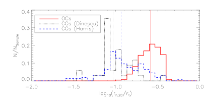
Figure 5: Top panel: The ratio $r_{h,\rm 2D}/r_{t}$ for OCs and GCs today for the 236 OCs of the sample by Piskunov et al. (2007), the 34 GCs of the sample by Dinescu et al. (1999) and 156 GCs of the Harris catalogue (Harris, 1996, 2010 edition). Note that $r_{h}=r_{\rm h,2D}$ is in this Figure the projected half-mass radius (OCs) or the half-light radius (GCs) given in the Harris catalogue, respectively. The vertical lines denote the medians.

Figure 5 shows the ratio $r_{h,\rm 2D}/r_{t}$ for OCs and GCs today for the 236 OCs of the sample by Piskunov et al. (2007), the 34 GCs of the sample by Dinescu et al. (1999) and 156 GCs of the Harris catalogue (Harris, 1996, 2010 edition). Note that $r_{h}=r_{\rm h,2D}$ is the projected half-mass radius (OCs) or the half-light radius (GCs) given in the Harris catalogue (Harris, 1996, 2010 edition), respectively. The vertical lines denote the medians.

We find the medians $\langle r_{t}/r_{h}\rangle=\langle\widehat{\lambda}/\lambda\rangle\approx 3.9$ (OCs), $\langle r_{t}/r_{h}\rangle\approx 11.0$ (Dinescu GCs), $\langle r_{t}/r_{h}\rangle\approx 8.7$ (Harris GCs). Therefore, with respect to this ratio, the average OC corresponds to a King model with low $W_{0}$ while the average GC corresponds to a King model with high $W_{0}$ according to Table 1 in Guerkan et al. (2004). We remark that the projected (2D) half-mass radius $r_{h}=r_{\rm h,2D}$ is larger than the 3D half-mass radius $r_{\rm h,3D}$. For the Plummer model $r_{\rm h,3D}/r_{\rm h,2D}\approx 1.30$ can be obtained analytically.

Applying Eqns. (8) and (10) to the data we find that

$$\lambda_{\rm GC}<\lambda_{\rm OC},\ \ \ \widehat{\lambda}_{\rm GC}<\widehat{\lambda}_{\rm OC}.$$ (22)

for an “average” GC and an “average” OC, with proportionality factors

$$\mu=\frac{\lambda_{\rm OC}}{\lambda_{\rm GC}},\ \ \ \widehat{\mu}=\frac{\widehat{\lambda}_{\rm OC}}{\widehat{\lambda}_{\rm GC}}$$ (23)

with $\mu\approx 5.4$ today and $\widehat{\mu}\approx 1.7$ today from the median values of crossing and orbital times given in Tables 1, 2 and 3. The isothermal approximation $\beta_{C}=\sqrt{2}$ was used.

The relative error in $\mu$ is given by

$$\frac{\Delta\mu}{\mu} = \sqrt{\left(\frac{\Delta\lambda_{\rm OC}}{\lambda_{\rm OC}}\right)^{2}+\left(\frac{\Delta\lambda_{\rm GC}}{\lambda_{\rm GC}}\right)^{2}}$$

$$= \ln(10)\sqrt{\left[\frac{\Delta\log_{10}\lambda_{\rm OC}}{\sqrt{N_{\rm OCs}}}\right]^{2}+\left[\frac{\Delta\log_{10}\lambda_{\rm GC}}{\sqrt{N_{\rm GCs}}}\right]^{2}}$$

$$\lesssim \ln(10)\sqrt{\left[\frac{(Q_{90}-Q_{10})_{\rm OCs}}{\sqrt{N_{\rm OCs}}}\right]^{2}+\left[\frac{(Q_{90}-Q_{10})_{\rm GCs}}{\sqrt{N_{\rm GCs}}}\right]^{2}}$$

The last line containing the 10 and 90 percent quantiles of the $\log_{10}\lambda$-distributions serves as an upper limit to the error. We obtain $\Delta\mu/\mu\lesssim 0.23$ for the upper limit.

We further remark that taking $t_{\rm cr,OC}/2$ instead of $t_{\rm cr,OC}$ in Eqn. (8) with all other quantities kept the same leads to $\mu\approx 3.4$ implying at least a $3\sigma$ confidence provided that there is no bias due to systematic errors (see discussion).

5 Discussion and conclusions

The results of the present study are as follows:

1. We found under the assumptions stated below that GCs are generally Roche volume underfilling in terms of $\widehat{\lambda}=r_{\mathrm{t}}/r_{\mathrm{J}}$. In the pericenters of their orbits a significant fraction might be Roche volume overfilling dependent on the dynamical compression of the outer shells compared to the smaller Jacobi radius.

2. We found under the assumptions stated below with at least $3\sigma$ confidence that the ratio $\lambda=r_{h}/r_{J}$ of half-mass and Jacobi radius is tendentially larger for an average open cluster within the nearest kpc of the Sun than for an average globular cluster and quantified the proportionality factor

   $$\mu=\left(\frac{r_{h}}{r_{J}}\right)_{\rm OCs}\Big{/}\left(\frac{r_{h}}{r_{J}}\right)_{\rm GCs}\approx 3-5.$$ (25)

3. The difference between OCs and GCs seems to be that, with respect to the concentration, the average OC has low concentration while the average GC has a high concentration.

4. A fraction of OCs may be Roche volume overfilling. However, the simple assumption of virial equilibrium breaks down for Roche volume overfilling clusters.

5. A closer inspection of Baumgardt et al. (2010) suggests that there is a physically extended subsample of low mass GCs with $r_{\mathrm{h}}>10$ pc, which may represent the post core collapse sequence of dissolving clusters. Our sample of GCs with known orbits is too small to confirm this scenario.

We make the following remarks:

1. The fact that $\lambda_{\rm GC}\ll 1$ explains (i) why GCs are spherically shaped as compared to the often irregularly shaped OCs, (ii) why GCs are stable against dissolution over a Hubble time and (iii) why not many GC tidal tails have been found observationally.

2. A fraction of OCs may be Roche volume overfilling ($\lambda_{\rm OC}>1$) at the time of their formation, but the shear forces of the tidal field will rapidly remove the material outside the Jacobi radius.

3. Only if the star cluster is in virial equilibrium Eqn. (5) is valid. Therefore the correlation found by van den Bergh (1994) suggests that an average GC is in virial equilibrium if we postulate that a constant ratio $\lambda_{\rm GC}$ is reasonable with respect to the general structure of GCs. We emphasize that the virial theorem cannot be valid for Roche volume overfilling clusters.

We rely on the following assumptions, stated in order of importance according to our view:

1. That the orbits of GCs in the sample of Dinescu et al. (1999) can be approximated by orbits in a purely isothermal halo for which the total angular momentum is conserved.

2. That the orbits of OCs can be approximated by circular orbits (for orbit calculations of OCs see, e.g., Cararro & Chiosi, 1994).

3. That there are no selection effects concerning the GC sample, i.e. the sample of GCs in Dinescu et al. (1999) is representative for the GC population of the Milky Way.

4. That the half-light and projected half-mass radii coincide.

5. That the velocity dispersion of OCs is not too much biased due to the presence of binaries.

It is crucial to this investigation whether the approximations (i) and (ii) are justified. In the future, our results may be falsified or improved towards higher confidence levels when more and better data are available.

Our investiation suggests that most GCs were formed deep in their potential well, i.e. Roche volume underfilling in contrast to OCs, which can be even Roche volume overfilling after gas expulsion. In future work we plan to investigate the dynamical reasoning for these intrinsic differences and to quantify the impact on the dissolution process of the star clusters.

6 Acknowledgements

AE is grateful for support by grant JU 404/3-1 of the German Research Foundation (DFG) and thanks Prof. Dr. Eva Grebel for a comment made during a talk which directed his interest to the van-den-Bergh correlation. Discussions with Prof. Dr. Rainer Spurzem are gratefully acknowledged and the fact, that the idea to Eqn. (8) was first written down on a notepad of him. Both authors thank the referee for the thoughtful comments.

Appendix A The ratio $\beta_{C}$

For any galactic potential $\Phi$, the dimensionless ratio $\beta_{C}=\kappa_{C}/\Omega_{C}$ is given by

$$\beta_{C}^{2}=2\left(1+\frac{d\ln V_{C}}{d\ln R}\right)\Big{|}_{R_{C}}=3+R\frac{\left(d^{2}\Phi/dR^{2}\right)}{\left(d\Phi/dR\right)}\Big{|}_{R_{C}}$$ (26)

where $\kappa_{C}$ and $\Omega_{C}$ are the epicyclic and circular frequency related to a circular orbit, $R_{C}$ is its radius and $V_{C}=\Omega_{C}R_{C}$ is the circular velocity at that radius. Figure 1 shows that $\beta_{C}$ is approximately constant for a wide range of Galactocentric radii for three different analytic Milky Way potentials, among them that two models used in Dinescu et al. (1999).

Appendix B Eccentric orbits

B.1 Kepler case

If we approximate the Milky Way potential by a Kepler potential $\Phi_{K}\propto r^{-1}$ we find $\beta_{C,K}=1$. Apo- and pericenter are defined by $R_{P}=a(1-e)$ and $R_{A}=a(1+e)$ where $a$ and $e$ are the semimajor axis and the eccentricity of the orbit. Also, we have the relation (c.f. King 1962, BT2008)

$$L^{2}=\Omega^{2}R^{4}=GM_{g}a(1-e^{2})=\frac{GM_{g}}{a}R_{A}R_{P},\ \ \$$ (27)

where $M_{g},\Omega$ and $R$ are the mass of the point-like galaxy, the angular speed and the galactocentric radius at any orbital phase, respectively.

With the gravitational potential and its derivatives

$$\Phi=-\frac{GM_{g}}{R},\ \ \ \frac{d\Phi}{dR}=\frac{GM_{g}}{R^{2}},\ \ \ \frac{d^{2}\Phi}{dR^{2}}=-\frac{2GM_{g}}{R^{3}}$$ (28)

we obtain the Jacobi radius

$$r_{J} = \left[\frac{GM_{cl}}{\Omega^{2}-\frac{d^{2}\Phi}{dR^{2}}}\right]^{1/3}$$ (29)

$$= \left(\frac{M_{\rm cl}}{M_{g}}\right)^{1/3}\left(\frac{aR^{4}}{R_{A}R_{P}+2aR}\right)^{1/3}$$ (30)

for circular and eccentric orbits (cf. King 1962).

B.2 Isothermal case

If we approximate the Milky Way potential by the potential of an isothermal sphere $\Phi_{I}=V_{C}^{2}\ln(R/R_{0})$ with the circular velocity $V_{C}$ we find $\beta_{C,I}=\sqrt{2}$ (note that the isothermal sphere has a constant rotation curve).

The energy (say, of a globular cluster) in an isothermal sphere is given by

$$E=\frac{V^{2}}{2}+V_{C}^{2}\ln\left(\frac{R}{R_{0}}\right)$$ (31)

where $R_{0}$ is a lenght unit. This yields

$$V^{2} = 2\left[E-V_{C}^{2}\ln\left(\frac{R}{R_{0}}\right)\right]$$ (32)

$$= 2V_{C}^{2}\ln\left[\exp(E/V_{C}^{2})\left(\frac{R_{0}}{R}\right)\right]=2V_{C}^{2}\ln\left(\frac{R_{0}^{\prime}}{R}\right)$$

with $R_{0}^{\prime}=\exp(E/V_{C}^{2})R_{0}$. For simplicity we substitute in the following discussion $R_{0}^{\prime}\rightarrow R_{0}$.

From the angular momentum conservation we obtain at apo- and pericentre

$$R_{P}^{2}\ln(R_{0}/R_{P})=R_{A}^{2}\ln(R_{0}/R_{A}).$$ (33)

From the energy conservation we obtain

$$\frac{V_{P}^{2}}{2}+V_{C}^{2}\ln\left(\frac{R_{P}}{R_{0}}\right)=\frac{V_{A}^{2}}{2}+V_{C}^{2}\ln\left(\frac{R_{A}}{R_{0}}\right)$$ (34)

We also obtain

$$V_{P}^{2}-V_{A}^{2}=2V_{C}^{2}\ln(R_{A}/R_{P})$$ (35)

The angular momentum as a function of $R_{A}$ and $R_{P}$ is given by

$$L=V_{C}R_{P}R_{A}\sqrt{\frac{2\ln(R_{A}/R_{P})}{R_{A}^{2}-R_{P}^{2}}}$$ (36)

The limiting cases are circular and radial orbits. Using $L^{2}$ we have verified (1) with the rule of l’Hospital that the Eqn. (36) is consistent with the limiting case of a circular orbit with radius $R_{C}$ and velocity $V_{C}$ and (2) that the radial orbit has zero angular momentum. From Eqn. (36) follows the relation

$$L^{2}=\Omega^{2}R^{4}=2V_{C}^{2}R_{P}^{2}R_{A}^{2}\frac{\ln(R_{A}/R_{P})}{R_{A}^{2}-R_{P}^{2}}$$ (37)

where $\Omega$ is the angular velocity at any orbital radius $R$. We follow now the derivation of $r_{J}$ in King (1962) for the case of an isothermal sphere. The gravitational potential of the isothermal sphere and its derivatives are given by

$$\Phi=V_{C}^{2}\ln\left(\frac{R}{R_{0}}\right),\ \ \ \ \ \frac{d\Phi}{dR}=\frac{V_{C}^{2}}{R},\ \ \ \ \ \frac{d^{2}\Phi}{dR^{2}}=-\frac{V_{C}^{2}}{R^{2}}.$$ (38)

We obtain for the Jacobi radius

$$r_{J}^{3} = \frac{GM_{cl}}{\Omega^{2}-\frac{d^{2}\Phi}{dR^{2}}}$$ (39)

$$= \frac{GM_{cl}(R_{A}^{2}-R_{P}^{2})R^{4}}{2V_{C}^{2}R_{P}^{2}R_{A}^{2}\ln(R_{A}/R_{P})+V_{C}^{2}(R_{A}^{2}-R_{P}^{2})R^{2}}$$ (40)

for circular and eccentric orbits (cf. King 1962).

If we define a “guiding radius”

$$R_{g}=\frac{L}{V_{C}}$$ (41)

the Jacobi radius can be written as

$$r_{J}=r_{v}^{1/3}\left(\frac{R^{4}}{R_{g}^{2}+R^{2}}\right)^{1/3}$$ (42)

where $r_{v}=GM_{cl}/V_{\rm C}^{2}$ is the velocity radius given by Eqn. (4) with the constant $V_{C}$ of the isothermal sphere. We also obtain

$$\lambda_{\rm I}=\left(\frac{r_{h}}{r_{J}}\right)_{\rm I}=\left(\frac{t_{\rm orb}}{2\pi}\right)^{2/3}\left(\frac{V_{C}}{\sqrt{2}R(t)}\right)^{2/3}\left(1+\frac{R_{g}^{2}}{R(t)^{2}}\right)^{1/3}.$$ (43)

where $R(t)$ is time-dependent for an accentric orbit.

B.3 Harmonic case

In the case of a sphere with homogeneous density $\rho_{0}$ we have $\beta_{\rm C,H}=2$ and $\Omega=\sqrt{4\pi G\rho_{0}/3}$ which is independent of $R$. Both the Jacobi radius in Eqn. (7) and the ratio in Eqn. (8) are not well defined.

B.4 Beyond the solar circle

Figure 6: The ratio $r_{h,\rm 3D}/r_{J}$ of GCs today calculated from Eqn. (10) for 17 GCs out of the 34 GCs in the sample by Dinescu et al. (1999) for which $R>8$ kpc under the assumption that the GCs are moving in an isothermal halo with $V_{C}\approx 228.5$ km/s and that the van-den-Bergh correlation holds.

Baumgardt et al. (2010) show that clusters with galactocentric distances $R>8$ kpc fall into two distinct groups: one group of compact, tidally-underfilling clusters with $r_{h}/r_{J}<$ 0.05 and another group of tidally filling clusters which have $0.1<r_{h}/r_{J}<0.3$. In Figure 6 we calculated the ratio $r_{h,\rm 3D}/r_{J}$ of GCs today from Eqn. (10) for 17 GCs out of the 34 GCs in the sample by Dinescu et al. (1999) for which $R>8$ kpc under the assumption that the GCs are moving in an isothermal halo with $V_{C}\approx 228.5$ km/s as in Figure 4. We do not clearly see the dichotomy in Figure 6. The reason may be that the Dinescu et al. (1999) data set is not large enough.

However, Baumgardt et al. (2010) argued about the case of NGC 2419, where the best-fitting King model has a tidal radius of 150 pc, while the estimated Jacobi radius of the cluster is around 800 pc (derived in Baumgardt et al. 2009). From our point of view this is a perfect case of a GC embedded deeply in its own potential well, such that a King model of an isolated cluster is a very good approximation, because the tidal field is negligible for the cluster.

References

- Baumgardt et al. (2009) Baumgardt H., et al., 2009, MNRAS, 396, 2051
- Baumgardt et al. (2010) Baumgardt H., Parmentier, G., Gieles, M., Vesperini, E., 2010, MNRAS, 401,1832
- Binney & Tremaine (2008) Binney J., Tremaine, S., 2008, Galactic dynamics, nd ed., Princeton University Press, Princeton
- Bonatto & Bica (2011) Bonatto, C., Bica, E., 2011, MNRAS, 415, 2827
- Cararro & Chiosi (1994) Carraro, G., Chiosi, C., 1994, A&A, 288, 751
- Converse & Stahler (2010) Converse, J. M., Stahler, S. W., 2010, MNRAS 405, 666
- Dinescu et al. (1999) Dinescu D. I., Girard T. M., Altena W. F., 1999, AJ, 117, 1792
- Ernst et al. (2010) Ernst A., Just, A., Berczik, P., Petrov, M.I., 2010, A&A 524, A62
- Guerkan et al. (2004) Gürkan, A., Freitag, M., Rasio, F. A., 2004, Ap. J., 604, 632
- Harris (1996, 2010 edition) Harris, W.E. 2012, arXiv:1012.3224
- Hong et al. (2004) Hong, J., Schlegel, E. M., Grindlay, J.E., 2004, Ap. J., 614, 508
- Johnston et al. (1995) Johnston, K. V., Spergel, D. N., Hernquist, L., 1995, Ap. J., 451, 598 (JSH95)
- Just et al. (2009) Just, A., Berczik, P., Petrov, M.I., Ernst, A., 2009, MNRAS 392, 969
- Kharchenko et al. (2009) Kharchenko N. V., Berczik P., Petrov M. I., Piskunov A. E., Röser S., Schilbach E., Scholz R.-D. 2009, A&A, 495, 807
- King (1962) King I. R., 1962, AJ, 67, 471
- Kroupa (2001) Kroupa, P., 2001, MNRAS, 322, 231
- Küpper et al. (2008) Küpper A. H. W., Macleod A., Heggie D. C., 2008, MNRAS, 387, 1248
- Lamers & Gieles (2006) Lamers, H. J. G. L. M.,Gieles, M., 2006, A&A 455, L17
- Ortolani et al. (2012) Ortolani, S., Bonatto, C., Bica, E., Barbuy, B., Saito, R. K., 2012, AJ, 144, 147
- Paczyński (2011) Paczyński, B., 1990, Ap. J., 348, 485 (P90)
- Piskunov et al. (2006) Piskunov, A. E., Kharchenko, N. V., Röser, S., Schilbach, E., Scholz, R.-D., 2006, A&A, 445, 545
- Piskunov et al. (2007) Piskunov, A. E., Schilbach, E., Kharchenko, N. V., Röser, S., Scholz, R.-D., 2007, A&A, 468, 151
- van den Bergh (1994) van den Bergh, S., 1994, AJ, 108, 2145