Geo-Indistinguishability: Differential Privacy for Location-Based Systems

Abstract

The growing popularity of location-based systems, allowing unknown/untrusted servers to easily collect huge amounts of information regarding users’ location, has recently started raising serious privacy concerns. In this paper we introduce geo-indistinguishability, a formal notion of privacy for location-based systems that protects the user’s exact location, while allowing approximate information – typically needed to obtain a certain desired service – to be released.

This privacy definition formalizes the intuitive notion of protecting the user’s location within a radius $r$ with a level of privacy that depends on $r$, and corresponds to a generalized version of the well-known concept of differential privacy. Furthermore, we present a mechanism for achieving geo-indistinguishability by adding controlled random noise to the user’s location.

We describe how to use our mechanism to enhance LBS applications with geo-indistinguishability guarantees without compromising the quality of the application results. Finally, we compare state-of-the-art mechanisms from the literature with ours. It turns out that, among all mechanisms independent of the prior, our mechanism offers the best privacy guarantees.

1 Introduction

In recent years, the increasing availability of location information about individuals has led to a growing use of systems that record and process location data, generally referred to as “location- based systems”. Such systems include (a) Location Based Services (LBSs), in which a user obtains, typically in real-time, a service related to his current location, and (b) location-data mining algorithms, used to determine points of interest and traffic patterns.

The use of LBSs, in particular, has been significantly increased by the growing popularity of mobile devices equipped with GPS chips, in combination with the increasing availability of wireless data connections. A resent study in the US shows that in $2012$, $46\%$ of the adult population of the country owns a smartphone and, furthermore, that $74\%$ of those owners use LBSs [1]. Examples of LBSs include mapping applications (e.g., Google Maps), Points of Interest (POI) retrieval (e.g., AroundMe), coupon/discount providers (e.g., GroupOn), GPS navigation (e.g., TomTom), and location-aware social networks (e.g., Foursquare).

While location-based systems have demonstrated to provide enormous benefits to individuals and society, the growing exposure of users’ location information raises important privacy issues. First of all, location information itself may be considered as sensitive. Furthermore, it can be easily linked to a variety of other information that an individual usually wishes to protect: by collecting and processing accurate location data on a regular basis, it is possible to infer an individual’s home or work location, sexual preferences, political views, religious inclinations, etc. In its extreme form, monitoring and control of an individual’s location has been even described as a form of slavery [12].

Several notions of privacy for location-based systems have been proposed in the literature. In Section 2 we give an overview of such notions, and we discuss their shortcomings in relation to our motivating LBS application. Aiming at addressing these shortcomings, we propose a formal privacy definition for LBSs, as well as a randomized technique that allows a user to disclose enough location information to obtain the desired service, while satisfying the aforementioned privacy notion. Our proposal is based on a generalization of differential privacy [14] developed in [8]. Like differential privacy, our notion and technique abstract from the side information of the adversary, such as any prior probabilistic knowledge about the user’s actual location.

As a running example, we consider a user located in Paris who wishes to query an LBS provider for nearby restaurants in a private way, i.e., by disclosing some approximate information $z$ instead of his exact location $x$. A crucial question is: what kind of privacy guarantee can the user expect in this scenario? To formalize this notion, we consider the level of privacy within a radius. We say that the user enjoys $\ell$-privacy within $r$ if, any two locations at distance at most $r$ produce observations with “similar” distributions, where the “level of similarity” depends on $\ell$. The idea is that $\ell$ represents the user’s level of privacy for that radius: the smaller $\ell$ is, the higher is the privacy.

In order to allow the LBS to provide a useful service, we require that the (inverse of the) level of privacy $\ell$ depend on the radius $r$. In particular, we require that it is proportional to $r$, which brings us to our definition of geo-indistinguishability:

A mechanism satisfies $\epsilon$-geo-indistinguishability iff for any radius $r>0$, the user enjoys $\epsilon r$-privacy within $r$.

This definition implies that the user is protected within any radius $r$, but with a level $\ell=\epsilon r$ that increases with the distance. Within a short radius, for instance $r\!=\!1$ km, $\ell$ is small, guaranteeing that the provider cannot infer the user’s location within, say, the 7th arrondissement of Paris. Farther away from the user, for instance for $r=1000$ km, $\ell$ becomes large, allowing the LBS provider to infer that with high probability the user is located in Paris instead of, say, London. Figure 1 illustrates the idea of privacy levels decreasing with the radius.

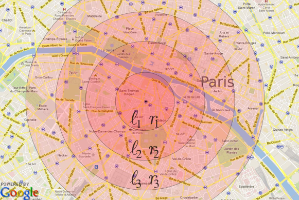
Figure 1: Geo-indistinguishability: privacy varying with $r$.

We develop a mechanism to achieve geo-indistinguishability by perturbating the user’s location $x$. The inspiration comes from one of the most popular approaches for differential privacy, namely the Laplacian noise. We adopt a specific planar version of the Laplace distribution, allowing to draw points in a geo-indistinguishable way; moreover, we are able to do so efficiently, via a transformation to polar coordinates. However, as standard (digital) applications require a finite representation of locations, it is necessary to add a discretization step. Such operation jeopardizes the privacy guarantees, for reasons similar to the rounding effects of finite-precision operations [29]. We show how to preserve geo-indistinguishability, at the price of a degradation of the privacy level, and how to adjust the privacy parameters in order to obtain a desired level of privacy.

We then describe how to use our mechanism to enhance LBS applications with geo-indistinguishability guarantees. Our proposal results in highly configurable LBS applications, both in terms of privacy and accuracy (a notion of utility/quality-of-service for LBS applications providing privacy via location perturbation techniques). Enhanced LBS applications require extra bandwidth consumption in order to provide both privacy and accuracy guarantees, thus we study how the different configurations affect the bandwidth overhead using the Google Places API [2] as reference to measure bandwidth consumption. Our experiments showed that the bandwidth overhead necessary to enhance LBS applications with very high levels of privacy and accuracy is not-prohibitive and, in most cases, negligible for modern applications.

Finally, we compare our mechanism with other ones in the literature, using the privacy metric proposed in [36]. It turns our that our mechanism offers the best privacy guarantees, for the same utility, among all those which do not depend on the prior knowledge of the adversary. The advantages of the independence from the prior are obvious: first, the mechanism is designed once and for all (i.e. it does not need to be recomputed every time the adversary changes, it works also in simultaneous presence of different adversaries, etc.). Second, and even more important, it is applicable also when we do not know the prior.

Contribution

This paper contributes to the state-of-the-art as follows:

• We show that our generalized notion of differential privacy [8], instantiated with the Euclidean metric, can be naturally applied to location privacy, and we discuss the privacy guarantees that this definition provides. (Location privacy was only briefly mentioned in [8] as a possible application.)

• We also extend it to location traces, using the ${d_{\infty}}$ metric, and show how privacy degrades when traces become longer.

• We propose a mechanism to efficiently draw noise from a planar Laplace distribution, which is not trivial. Laplacians on general metric spaces were briefly discussed in [8], but no efficient method to draw from them was given. Furthermore, we cope with the crucial problems of discretization and truncation, which have been shown to pose significant threats to mechanism implementations [29].

• We describe how to use our mechanism to enhance LBS applications with geo-indistinguishability guarantees.

• We compare our mechanism to a state-of-the-art mechanism from the literature [36] as well as a simple cloaking mechanism, obtaining favorable results.

Road Map

In Section 2 we discuss notions of location privacy from the literature and point out their weaknesses and strengths. In Section 3 we formalize the notion of geo-indistinguishability in three equivalent ways. We then proceed to describe a mechanism that provides geo-indistinguishability in Section 4. In Section 5 we show how to enhance LBS applications with geo-indistinguishability guarantees. In Section 6 we compare the privacy guarantees of our methods with those of two other methods from the literature. Section 7 discusses related work and Section 8 concludes.

The interested reader can find the proofs in the report version of this paper [4], which is available online.

2 Existing Notions of Privacy

In this section, we examine various notions of location privacy from the literature, as well as techniques to achieve them. We consider the motivating example from the introduction, of a user in Paris wishing to find nearby restaurants with good reviews. To achieve this goal, he uses a handheld device (e.g.. a smartphone) to query a public LBS provider. However, the user expects his location to be kept private: informally speaking, the information sent to the provider should not allow him to accurately infer the user’s location. Our goal is to provide a formal notion of privacy that adequately captures the user’s expected privacy. From the point of view of the employed mechanism, we require a technique that can be performed in real-time by a handheld device, without the need of any trusted anonymization party.

Expected Distance Error

Expectation of distance error [35, 36, 23] is a natural way to quantify the privacy offered by a location-obfuscation mechanism. Intuitively, it reflects the degree of accuracy by which an adversary can guess the real location of the user by observing the obfuscated location, and using the side-information available to him.

There are several works relying on this notion. In [23], a perturbation mechanism is used to confuse the attacker by crossing paths of individual users, rendering the task of tracking individual paths challenging. In [36], an optimal location-obfuscation mechanism (i.e., achieving maximum level of privacy for the user) is obtained by solving a linear program in which the contraints are determined by the quality of service and by the user’s profile.

It is worth noting that this privacy notion and the obfuscation mechanisms based on it are explicitly defined in terms of the adversary’s side information. In contrast, our notion of geo-indistinguishability abstracts from the attacker’s prior knowledge, and is therefore suitable for scenarios where the prior is unknown, or the same mechanism must be used for multiple users. A detailed comparison with the mechanism of [36] is provided in Section 6.

$k$-anonymity

The notion of $k$-anonymity is the most widely used definition of privacy for location-based systems in the literature. Many systems in this category [21, 19, 30] aim at protecting the user’s identity, requiring that the attacker cannot infer which user is executing the query, among a set of $k$ different users. Such systems are outside the scope of our problem, since we are interested in protecting the user’s location.

On the other hand, $k$-anonymity has also been used to protect the user’s location (sometimes called $l$-diversity in this context), requiring that it is indistinguishable among a set of $k$ points (often required to share some semantic property). One way to achieve this is through the use of dummy locations [25, 33]. This technique involves generating $k-1$ properly selected dummy points, and performing $k$ queries to the service provider, using the real and dummy locations. Another method for achieving $k$-anonymity is through cloaking [6, 13, 38]. This involves creating a cloaking region that includes $k$ points sharing some property of interest, and then querying the service provider for this cloaking region.

Even when side knowledge does not explicitly appear in the definition of $k$-anonymity, a system cannot be proven to satisfy this notion unless assumptions are made about the attacker’s side information. For example, dummy locations are only useful if they look equally likely to be the real location from the point of view of the attacker. Any side information that allows to rule out any of those points, as having low probability of being the real location, would immediately violate the definition.

Counter-measures are often employed to avoid this issue: for instance, [25] takes into account concepts such as ubiquity, congestion and uniformity for generating dummy points, in an effort to make them look realistic. Similarly, [38] takes into account the user’s side information to construct a cloaking region. Such counter-measures have their own drawbacks: first, they complicate the employed techniques, also requiring additional data to be taken into account (for instance, precise information about the environment or the location of nearby users), making their application in real-time by a handheld device challenging. Moreover, the attacker’s actual side information might simply be inconsistent with the assumptions being made.

As a result, notions that abstract from the attacker’s side information, such as differential privacy, have been growing in popularity in recent years, compared to $k$-anonymity-based approaches.

Differential Privacy

Differential Privacy [14] is a notion of privacy from the area of statistical databases. Its goal is to protect an individual’s data while publishing aggregate information about the database. Differential privacy requires that modifying a single user’s data should have a negligible effect on the query outcome. More precisely, it requires that the probability that a query returns a value $v$ when applied to a database $D$, compared to the probability to report the same value when applied to an adjacent database $D^{\prime}$ – meaning that $D,D^{\prime}$ differ in the value of a single individual – should be within a bound of $e^{\epsilon}$. A typical way to achieve this notion is to add controlled random noise to the query output, for example drawn from a Laplace distribution. An advantage of this notion is that a mechanism can be shown to be differentially private independently from any side information that the attacker might possess.

Differential privacy has also been used in the context of location privacy. In [28], it is shown that a synthetic data generation technique can be used to publish statistical information about commuting patterns in a differentially private way. In [22], a quadtree spatial decomposition technique is used to ensure differential privacy in a database with location pattern mining capabilities.

As shown in the aforementioned works, differential privacy can be successfully applied in cases where aggregate information about several users is published. On the other hand, the nature of this notion makes it poorly suitable for applications in which only a single individual is involved, such as our motivating scenario. The secret in this case is the location of a single user. Thus, differential privacy would require that any change in that location should have negligible effect on the published output, making it impossible to communicate any useful information to the service provider.

To overcome this issue, Dewri [11] proposes a mix of differential privacy and $k$-anonymity, by fixing an anonymity set of $k$ locations and requiring that the probability to report the same obfuscated location $z$ from any of these $k$ locations should be similar (up to $e^{\epsilon}$). This property is achieved by adding Laplace noise to each Cartesian coordinate independently. There are however two problems with this definition: first, the choice of the anonymity set crucially affects the resulting privacy; outside this set no privacy is guaranteed at all. Second, the property itself is rather weak; reporting the geometric median (or any deterministic function) of the $k$ locations would satisfy the same definition, although the privacy guarantee would be substantially lower than using Laplace noise.

Nevertheless, Dewri’s intuition of using Laplace noise for location privacy is valid, and [11] provides extensive experimental analysis supporting this claim. Our notion of geo-indistinguishability provides the formal background for justifying the use of Laplace noise, while avoiding the need to fix an anonymity set by using the generalized variant of differential privacy from [8].

Other location-privacy metrics

[10] proposes a location cloaking mechanism, and focuses on the evaluation of Location-based Range Queries. The degree of privacy is measured by the size of the cloak (also called uncertainty region), and by the coverage of sensitive regions, which is the ratio between the area of the cloak and the area of the regions inside the cloak that the user considers to be sensitive. In order to deal with the side-information that the attacker may have, ad-hoc solutions are proposed, like patching cloaks to enlarge the uncertainty region or delaying requests. Both solutions may cause a degradation in the quality of service.

In [5], the real location of the user is assumed to have some level of inaccuracy, due to the specific sensing technology or to the environmental conditions. Different obfuscation techniques are then used to increase this inaccuracy in order to achieve a certain level of privacy. This level of privacy is defined as the ratio between the accuracy before and after the application of the obfuscation techniques.

Similar to the case of $k$-anonymity, both privacy metrics mentioned above make implicit assumptions about the adversary’s side information. This may imply a violation of the privacy definition in a scenario where the adversary has some knowledge about the user’s real location.

Transformation-based approaches

A number of approaches for location privacy are radically different from the ones mentioned so far. Instead of cloaking the user’s location, they aim at making it completely invisible to the service provider. This is achieved by transforming all data to a different space, usually employing cryptographic techniques, so that they can be mapped back to spatial information only by the user [24, 20]. The data stored in the provider, as well as the location send by the user are encrypted. Then, using techniques from private information retrieval, the provider can return information about the encrypted location, without ever discovering which actual location it corresponds to.

A drawback of these techniques is that they are computationally demanding, making it difficult to implement them in a handheld device. Moreover, they require the provider’s data to be encrypted, making it impossible to use existing providers, such as Google Maps, which have access to the real data.

3 Geo-Indistinguishability

In this section we formalize our notion of geo-indistinguishability. As already discussed in the introduction, the main idea behind this notion is that, for any radius $r>0$, the user enjoys $\epsilon r$-privacy within $r$, i.e. the level of privacy is proportional to the radius. Note that the parameter $\epsilon$ corresponds to the level of privacy at one unit of distance. For the user, a simple way to specify his privacy requirements is by a tuple $(\ell,r)$, where $r$ is the radius he is mostly concerned with and $\ell$ is the privacy level he wishes for that radius. In this case, it is sufficient to require $\epsilon$-geo-indistinguishability for $\epsilon=\ell/r$; this will ensure a level of privacy $\ell$ within $r$, and a proportionally selected level for all other radii.

So far we kept the discussion on an informal level by avoiding to explicitly define what $\ell$-privacy within $r$ means. In the remaining of this section we give a formal definition, as well as two characterizations which clarify the privacy guarantees provided by geo-indistinguishability.

Probabilistic model

We first introduce a simple model used in the rest of the paper. We start with a set $\mathcal{X}$ of points of interest, typically the user’s possible locations. Moreover, let $\mathcal{Z}$ be a set of possible reported values, which in general can be arbitrary, allowing to report obfuscated locations, cloaking regions, sets of locations, etc. However, to simplify the discussion, we sometimes consider $\mathcal{Z}$ to also contain spatial points, assuming an operational scenario of a user located at $x\in\mathcal{X}$ and communicating to the attacker a randomly selected location $z\in\mathcal{Z}$ (e.g. an obfuscated point).

Probabilities come into place in two ways. First, the attacker might have side information about the user’s location, knowing, for example, that he is likely to be visiting the Eiffel Tower, while unlikely to be swimming in the Seine river. The attacker’s side information can be modeled by a prior distribution $\pi$ on $\mathcal{X}$, where $\pi(x)$ is the probability assigned to the location $x$.

Second, the selection of a reported value in $\mathcal{Z}$ is itself probabilistic; for instance, $z$ can be obtained by adding random noise to the actual location $x$ (a technique used in Section 4). A mechanism $K$ is a probabilistic function for selecting a reported value; i.e. $K$ is a function assigning to each location $x\in\mathcal{X}$ a probability distribution on $\mathcal{Z}$, where $K(x)(Z)$ is the probability that the reported point belongs to the set $Z\subseteq\mathcal{Z}$, when the user’s location is $x$. Starting from $\pi$ and using Bayes’ rule, each observation $Z\subseteq\mathcal{Z}$ of a mechanism $K$ induces a posterior distribution $\sigma=\mathbf{Bayes}(\pi,K,Z)$ on $\mathcal{X}$, defined as $\sigma(x)=\textstyle{\frac{K(x)(Z)\pi(x)}{\sum_{x^{\prime}}K(x^{\prime})(Z)\pi(x^{\prime})}}$.

We define the multiplicative distance between two distributions $\sigma_{1},\sigma_{2}$ on some set $\mathcal{S}$ as ${d_{\mathcal{P}}}(\sigma_{1},\sigma_{2})\allowbreak=\allowbreak\sup_{S\subseteq\mathcal{S}}|\ln\textstyle{\frac{\sigma_{1}(S)}{\sigma_{2}(S)}}|$, with the convention that $|\ln\textstyle{\frac{\sigma_{1}(S)}{\sigma_{2}(S)}}|=0$ if both $\sigma_{1}(S),\sigma_{2}(S)$ are zero and $\infty$ if only one of them is zero.

3.1 Definition

We are now ready to state our definition of geo-indistinguishability. Intuitively, a privacy requirement is a constraint on the distributions $K(x),K(x^{\prime})$ produced by two different points $x,x^{\prime}$. Let $d(\cdot,\cdot)$ denote the Euclidean metric. Enjoying $\ell$-privacy within $r$ means that for any $x,x^{\prime}$ s.t. $d(x,x^{\prime})\allowbreak\leq\allowbreak r$, the distance ${d_{\mathcal{P}}}(K(x),\allowbreak K(x^{\prime}))$ between the corresponding distributions should be at most $l$. Then, requiring $\epsilon r$-privacy for all radii $r$, forces the two distributions to be similar for locations close to each other, while relaxing the constraint for those far away from each other, allowing a service provider to distinguish points in Paris from those in London.

Definition 3.1 (geo-indistinguishability)

A mechanism $K$ satisfies $\epsilon$-geo-indistinguishability iff for all $x,x^{\prime}$:

$${d_{\mathcal{P}}}(K(x),K(x^{\prime}))\leq\epsilon d(x,x^{\prime})$$

Equivalently, the definition can be formulated as $K(x)(Z)\leq$ $\allowbreak e^{\epsilon d(x,x^{\prime})}\allowbreak K(x^{\prime})(Z)$ for all $x,x^{\prime}\in\mathcal{X},Z\subseteq\mathcal{Z}$. Note that for all points $x^{\prime}$ within a radius $r$ from $x$, the definition forces the corresponding distributions to be at most $\epsilon r$ distant.

The above definition is very similar to the one of differential privacy, which requires ${d_{\mathcal{P}}}(K(x),K(x^{\prime}))\leq\epsilon{d_{h}}(x,x^{\prime})$, where ${d_{h}}$ is the Hamming distance between databases $x,x^{\prime}$, i.e. the number of individuals in which they differ. In fact, geo-indistinguishability is an instance of a generalized variant of differential privacy, using an arbitrary metric between secrets. This generalized formulation has been known for some time: for instance, [31] uses it to perform a compositional analysis of standard differential privacy for functional programs, while [16] uses metrics between individuals to define “fairness” in classification. On the other hand, the usefulness of using different metrics to achieve different privacy goals and the semantics of the privacy definition obtained by different metrics have only recently started to be studied [8]. This paper focuses on location-based systems and is, to our knowledge, the first work considering privacy under the Euclidean metric, which is a natural choice for spatial data.

Note that in our scenario, using the Hamming metric of standard differential privacy – which aims at completely protecting the value of an individual – would be too strong, since the only information is the location of a single individual. Nevertheless, we are not interested in completely hiding the user’s location, since some approximate information needs to be revealed in order to obtain the required service. Hence, using a privacy level that depends on the Euclidean distance between locations is a natural choice.

A note on the unit of measurement

It is worth noting that, since $\epsilon$ corresponds to the privacy level for one unit of distance, it is affected by the unit in which distances are measured. For instance, assume that $\epsilon=0.1$ and distances are measured in meters. The level of privacy for points one kilometer away is $1000\epsilon$, hence changing the unit to kilometers requires to set $\epsilon=100$ in order for the definition to remain unaffected. In other words, if $r$ is a physical quantity expressed in some unit of measurement, then $\epsilon$ has to be expressed in the inverse unit.

3.2 Characterizations

In this section we state two characterizations of geo-indistinguishability, obtained from the corresponding results of [8] (for general metrics), which provide intuitive interpretations of the privacy guarantees offered by geo-indistinguishability.

Adversary’s conclusions under hiding

The first characterization uses the concept of a hiding function $\phi:\mathcal{X}\to\mathcal{X}$. The idea is that $\phi$ can be applied to the user’s actual location before the mechanism $K$, so that the latter has only access to a hidden version $\phi(x)$, instead of the real location $x$. A mechanism $K$ with hiding applied is simply the composition $K\circ\phi$. Intuitively, a location remains private if, regardless of his side knowledge (captured by his prior distribution), an adversary draws the same conclusions (captured by his posterior distribution), regardless of whether hiding has been applied or not. However, if $\phi$ replaces locations in Paris with those in London, then clearly the adversary’s conclusions will be greatly affected. Hence, we require that the effect on the conclusions depends on the maximum distance $d(\phi)\allowbreak=\sup_{x\in\mathcal{X}}d(x,\phi(x))$ between the real and hidden location.

Theorem 3.1

A mechanism $K$ satisfies $\epsilon$-geo-indistinguishability iff for all $\phi:\mathcal{X}\to\mathcal{X}$, all priors $\pi$ on $\mathcal{X}$, and all $Z\subseteq\mathcal{Z}$:

$${d_{\mathcal{P}}}(\sigma_{1},\sigma_{2}) \leq 2\epsilon d(\phi) \textrm{where}\qquad\sigma_{1} =\mathbf{Bayes}(\pi,K,Z)$$

$$\sigma_{2} =\mathbf{Bayes}(\pi,K\circ\phi,Z)$$

Note that this is a natural adaptation of a well-known interpretation of standard differential privacy, stating that the attacker’s conclusions are similar, regardless of his side knowledge, and regardless of whether an individual’s real value has been used in the query or not. This corresponds to a hiding function $\phi$ removing the value of an individual.

Note also that the above characterization compares two posterior distributions. Both $\sigma_{1},\sigma_{2}$ can be substantially different than the initial knowledge $\pi$, which means that an adversary does learn some information about the user’s location.

Knowledge of an informed attacker

A different approach is to measure how much the adversary learns about the user’s location, by comparing his prior and posterior distributions. However, since some information is allowed to be revealed by design, these distributions can be far apart. Still, we can consider an informed adversary who already knows that the user is located within a set $N\subseteq\mathcal{X}$. Let $d(N)=\sup_{x,x^{\prime}\in N}d(x,x^{\prime})$ be the maximum distance between points in $x$. Intuitively, the user’s location remains private if, regardless of his prior knowledge within $N$, the knowledge obtained by such an informed adversary should be limited by a factor depending on $d(N)$. This means that if $d(N)$ is small, i.e. the adversary already knows the location with some accuracy, then the information that he obtains is also small, meaning that he cannot improve his accuracy. Denoting by $\pi_{|N}$ the distribution obtained from $\pi$ by restricting to $N$ (i.e. $\pi_{|N}(x)=\pi(x|N)$), we obtain the following characterization:

Theorem 3.2

A mechanism $K$ satisfies $\epsilon$-geo-indistinguishability iff for all $N\subseteq\mathcal{X}$, all priors $\pi$ on $\mathcal{X}$, and all $Z\subseteq\mathcal{Z}$:

$${d_{\mathcal{P}}}(\pi_{|N},\sigma_{|N}) \leq\epsilon d(N) \textrm{where}\qquad\sigma =\mathbf{Bayes}(\pi,K,Z)$$

Note that this is a natural adaptation of a well-known interpretation of standard differential privacy, stating that in informed adversary who already knows all values except individual’s $i$, gains no extra knowledge from the reported answer, regardless of side knowledge about $i$’s value [17].

Abstracting from side information

A major difference of geo-indistinguishability, compared to similar approaches from the literature, is that it abstracts from the side information available to the adversary, i.e. from the prior distribution. This is a subtle issue, and often a source of confusion, thus we would like to clarify what “abstracting from the prior” means. The goal of a privacy definition is to restrict the information leakage caused by the observation. Note that the lack of leakage does not mean that the user’s location cannot be inferred (it could be inferred by the prior alone), but instead that the adversary’s knowledge does not increase due to the observation.

However, in the context of LBSs, no privacy definition can ensure a small leakage under any prior, and at the same time allow reasonable utility. Consider, for instance, an attacker who knows that the user is located at some airport, but not which one. The attacker’s prior knowledge is very limited, still any useful LBS query should reveal at least the user’s city, from which the exact location (i.e. the city’s airport) can be inferred. Clearly, due to the side information, the leakage caused by the observation is high.

So, since we cannot eliminate leakage under any prior, how can we give a reasonable privacy definition without restricting to a particular one? First, we give a formulation (Definition 3.1) which does not involve the prior at all, allowing to verify it without knowing the prior. At the same time, we give two characterizations which explicitly quantify over all priors, shedding light on how the prior affects the privacy guarantees.

Finally, we should point out that differential privacy abstracts from the prior in exactly the same way. Contrary to what is sometimes believed, the user’s value is not protected under any prior information. Recalling the well-known example from [14], if the adversary knows that Terry Gross is two inches shorter than the average Lithuanian woman, then he can accurately infer the height, even if the average is release in a differentially private way (in fact no useful mechanism can prevent this leakage). Differential privacy does ensure that her risk is the same whether she participates in the database or not, but this might me misleading: it does not imply the lack of leakage, only that it will happen anyway, whether she participates or not!

3.3 Protecting location sets

So far, we have assumed that the user has a single location that he wishes to communicate to a service provider in a private way (typically his current location). In practice, however, it is common for a user to have multiple points of interest, for instance a set of past locations or a set of locations he frequently visits. In this case, the user might wish to communicate to the provider some information that depends on all points; this could be either the whole set of points itself, or some aggregate information, for instance their centroid. As in the case of a single location, privacy is still a requirement; the provider is allowed to obtain only approximate information about the locations, their exact value should be kept private. In this section, we discuss how $\epsilon$-geo-indistinguishability extends to the case where the secret is a tuple of points $\mathbf{x}=(x_{1},\ldots,x_{n})$.

Similarly to the case of a single point, the notion of distance is crucial for our definition. We define the distance between two tuples of points $\mathbf{x}=(x_{1},\ldots,x_{n}),\mathbf{x}^{\prime}=(x_{1}^{\prime},\ldots,x_{n}^{\prime})$ as:

$${d_{\infty}}(\mathbf{x},\mathbf{x}^{\prime})=\textstyle{\max_{i}\>}d(x_{i},x_{i}^{\prime})$$

Intuitively, the choice of metric follows the idea of reasoning within a radius $r$: when ${d_{\infty}}(\mathbf{x},\mathbf{x}^{\prime})\leq r$, it means that all $x_{i},x_{i}^{\prime}$ are within distance $r$ from each other. All definitions and results of this section can be then directly applied to the case of multiple points, by using ${d_{\infty}}$ as the underlying metric. Enjoying $\ell$-privacy within a radius $r$ means that two tuples at most $r$ away from each other, should produce distributions at most $\epsilon r$ apart.

Reporting the whole set

A natural question then to ask is how we can obfuscate a tuple of points, by independently applying an existing mechanism $K_{0}$ to each individual point, and report the obfuscated tuple. Starting from a tuple $\mathbf{x}=(x_{1},\ldots,x_{n})$, we independently apply $K_{0}$ to each $x_{i}$ obtaining a reported point $z_{i}$, and then report the tuple $\mathbf{z}=(z_{1},\ldots,z_{n})$. Thus, the probability that the combined mechanism $K$ reports $\mathbf{z}$, starting from $\mathbf{x}$, is the product of the probabilities to obtain each point $z_{i}$, starting from the corresponding point $x_{i}$, i.e. $K(\mathbf{x})(\mathbf{z})=\prod_{i}K_{0}(x_{i})(z_{i})$.

The next question is what level of privacy does $K$ satisfy. For simplicity, consider a tuple of only two points $(x_{1},x_{2})$, and assume that $K_{0}$ satisfies $\epsilon$-geo-indistinguishability. At first look, one might expect the combined mechanism $K$ to also satisfy $\epsilon$-geo-indistinguishability, however this is not the case. The problem is that the two points might be correlated, thus an observation about $x_{1}$ will reveal information about $x_{2}$ and vice versa. Consider, for instance, the extreme case in which $x_{1}=x_{2}$. Having two observations about the same point reduces the level of privacy, thus we cannot expect the combined mechanism to provide the same level of privacy.

Still, if $K_{0}$ satisfies $\epsilon$-geo-indistinguishability, then $K$ can be shown to satisfy $n\epsilon$-geo-indistinguishability, i.e. a level of privacy that scales linearly with $n$. Due to this scalability issue, the technique of independently applying a mechanism to each point is only useful when the number of points is small. Still, this is sufficient for some applications, such as the case study of Section 5. Note, however, that this technique is by no means the best we can hope for: similarly to standard differential privacy [7, 32], better results could be achieved by adding noise to the whole tuple $\mathbf{x}$, instead of each individual point. We believe that using such techniques we can achieve geo-indistinguishability for a large number of locations with reasonable noise, leading to practical mechanisms for highly mobile applications. We have already started exploring this direction of future work.

Reporting an aggregate location

Another interesting case is when we need to report some aggregate information obtained by $\mathbf{x}$, for instance the centroid of the tuple. In general we might need to report the result of a query $f:\mathcal{X}^{n}\to\mathcal{X}$. Similarly to the case of standard differential privacy, we can compute the real answer $f(\mathbf{x})$ and the add noise by applying a mechanism $K$ to it. If $f$ is $\Delta$-sensitive wrt $d,{d_{\infty}}$, meaning that $d(f(\mathbf{x}),f(\mathbf{x}^{\prime}))\leq\Delta{d_{\infty}}(\mathbf{x},\mathbf{x}^{\prime})$ for all $\mathbf{x},\mathbf{x}^{\prime}$, and $K$ satisfies geo-indistinguishability, then the composed mechanism $K\circ f$ can be shown to satisfy $\Delta\epsilon$-geo-indistinguishability.

Note that when dealing with aggregate data, standard differential privacy becomes a viable option. However, one needs to also examine the loss of utility caused by the added noise. This highly depends on the application: differential privacy is suitable for publishing aggregate queries with low sensitivity, meaning that changes in a single individual have a relatively small effect on the outcome. On the other hand, location information often has high sensitivity. A trivial example is the case where we want to publish the complete tuple of points. But sensitivity can be high even for aggregate information: consider the case of publishing the centroid of 5 users located anywhere in the world. Modifying a single user can hugely affect their centroid, thus achieving differential privacy would require so much noise that the result would be useless. For geo-indistinguishability, on the other hand, one needs to consider the distance between points when computing the sensitivity. In the case of the centroid, a small (in terms of distance) change in the tuple has a small effect on the result, thus geo-indistinguishability can be achieved with much less noise.

4 A mechanism to achieve geo-indistinguishability

In this section we present a method to generate noise so to satisfy geo-indistinguishability. We model the location domain as a discrete Cartesian plane with the standard notion of Euclidean distance. This model can be considered a good approximation of the Earth surface when the area of interest is not too large.

1. First, we define a mechanism to achieve geo-indistinguishability in the ideal case of the continuous plane.

2. Then, we discretized the mechanism by remapping each point generated according to (a) to the closest point in the discrete domain.

3. Finally, we truncate the mechanism, so to report only points within the limits of the area of interest.

4.1 A mechanism for the continuous plane

Following the above plan, we start by defining a mechanism for geo-indistinguishability on the continuous plane. The idea is that whenever the actual location is ${x}_{0}\in\mathbb{R}^{2}$, we report, instead, a point ${x}\in\mathbb{R}^{2}$ generated randomly according to the noise function. The latter needs to be such that the probabilities of reporting a point in a certain (infinitesimal) area around ${x}$, when the actual locations are ${x}_{0}$ and ${x}^{\prime}_{0}$ respectively, differs at most by a multiplicative factor $e^{-\epsilon\,{d({x}_{0},{x}^{\prime}_{0})}}$.

We can achieve this property by requiring that the probability of generating a point in the area around ${x}$ decreases exponentially with the distance from the actual location ${x}_{0}$. In a linear space this is exactly the behavior of the Laplace distribution, whose probability density function (pdf) is $\nicefrac{{\epsilon}}{{2}}\,e^{-\epsilon\,|x-\mu|}$. This distribution has been used in the literature to add noise to query results on statistical databases, with $\mu$ set to be the actual answer, and it can be shown to satisfy $\epsilon$-differential privacy [15].

There are two possible definitions of Laplace distribution on higher dimensions (multivariate Laplacians). The first one, investigated in [27], and used also in [17], is obtained from the standard Laplacian by replacing $|x-\mu|$ with $d({x},{\mu})$. The second way consists in generating each Cartesian coordinate independently, according to a linear Laplacian. For reasons that will become clear in the next paragraph, we adopt the first approach.

The probability density function

Given the parameter $\epsilon\in\mathbb{R}^{+}$, and the actual location ${x}_{0}\in\mathbb{R}^{2}$, the pdf of our noise mechanism, on any other point ${x}\in\mathbb{R}^{2}$, is:

$$D_{\epsilon}({x}_{0})({x})=\frac{\epsilon^{2}}{2\,\pi}\,e^{-\epsilon\,{d({x}_{0},{x})}}$$ (1)

where $\nicefrac{{\epsilon^{2}}}{{2\,\pi}}$ is a normalization factor. We call this function planar Laplacian centered at ${x}_{0}$. The corresponding distribution is illustrated in Figure 2. It is possible to show that (i) the projection of a planar Laplacian on any vertical plane passing by the center gives a (scaled) linear Laplacian, and (ii) the corresponding mechanism satisfies $\epsilon$-geo-indistinguishability. These two properties would not be satisfied by the second approach to the multivariate Laplacian.

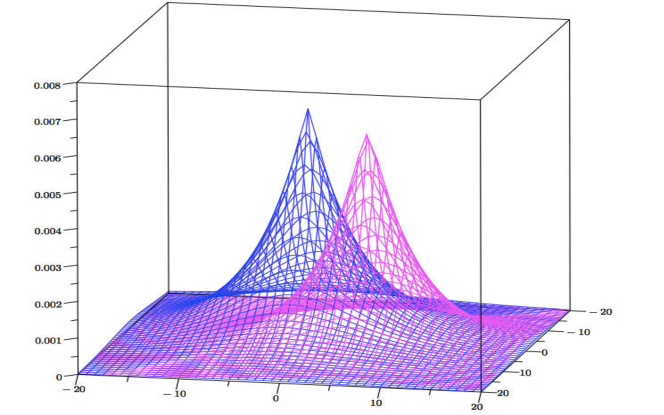
Figure 2: The pdf of two planar Laplacians, centered at $(-2,-4)$ and at $(5,3)$ respectively, with $\epsilon=1/5$.

Drawing a random point

We illustrate now how to draw a random point from the pdf defined in (1). First of all, we note that the pdf of the planar Laplacian depends only on the distance from ${x}_{0}$. It will be convenient, therefore, to switch to a system of polar coordinates with origin in ${x}_{0}$. A point ${x}$ will be represented as a point $(r,\theta)$, where $r$ is the distance of ${x}$ from ${x}_{0}$, and $\theta$ is the angle that the line ${x}\,{x}_{0}$ forms with respect to the horizontal axis of the Cartesian system. Following the standard transformation formula, the pdf of the polar Laplacian centered at the origin (${x}_{0}$) is:

$$D_{\epsilon}(r,\theta)=\frac{\epsilon^{2}}{2\,\pi}\,r\,e^{-\epsilon\,r}$$ (2)

We note now that the polar Laplacian defined above enjoys a property that is very convenient for drawing in an efficient way: the two random variables that represent the radius and the angle are independent. Namely, the pdf can be expressed as the product of the two marginals. In fact, let us denote these two random variables by $R$ (the radius) and $\Theta$ (the angle). The two marginals are:

$$\begin{array}[]{rcl}D_{\epsilon,R}(r)&=&\int_{0}^{2\pi}D_{\epsilon}(r,\theta)\,d\theta\,=\,\epsilon^{2}\,r\,e^{-\epsilon\,r}\\[8.61108pt] D_{\epsilon,\Theta}(\theta)&=&\int_{0}^{\infty}D_{\epsilon}(r,\theta)\,dr\,=\,\frac{1}{2\,\pi}\end{array}$$

Hence we have $D_{\epsilon}(r,\theta)=D_{\epsilon,R}(r)\;D_{\epsilon,\Theta}(\theta)$. Note that $D_{\epsilon,R}(r)$ corresponds to the pdf of the gamma distribution with shape $2$ and scale $1/\epsilon$.

Thanks to the fact that $R$ and $\Theta$ are independent, in order to draw a point $(r,\theta)$ from $D_{\epsilon}(r,\theta)$ it is sufficient to draw separately $r$ and $\theta$ from $D_{\epsilon,R}(r)$ and $D_{\epsilon,\Theta}(\theta)$ respectively.

Since $D_{\epsilon,\Theta}(\theta)$ is constant, drawing $\theta$ is easy: it is sufficient to generate $\theta$ as a random number in the interval $[0,2\pi)$ with uniform distribution.

We now show how to draw $r$. Following standard lines, we consider the cumulative distribution function (cdf) $C_{\epsilon}(r)$:

$$C_{\epsilon}(r)\,=\,\displaystyle\int_{0}^{r}D_{\epsilon,R}(\rho)d\rho\,=\,\displaystyle 1-(1+\epsilon\,r)\,e^{-\epsilon\,r}$$

Intuitively, $C_{\epsilon}(r)$ represents the probability that the radius of the random point falls between $0$ and $r$. Finally, we generate a random number $p$ with uniform probability in the interval $[0,1)$, and we set $r=C_{\epsilon}^{-1}(p)$. Note that

$$C_{\epsilon}^{-1}(p)=-\textstyle{\frac{1}{\epsilon}}\big{(}W_{\!\!-1}(\textstyle{\frac{p-1}{e}})+1\big{)}$$

where $W_{\!\!-1}$ is the Lambert W function (the $-1$ branch), which can be computed efficiently and is implemented in several numerical libraries (MATLAB, Maple, GSL, …).

4.2 Discretization

We discuss now how to approximate the Laplace mechanism on a grid $\mathcal{G}$ of discrete Cartesian coordinates. Let us recall the points (a) and (b) of the plan, in light of the development so far: Given the actual location ${x}_{0}$, report the point ${x}$ in $\mathcal{G}$ obtained as follows:

1. first, draw a point $(r,\theta)$ following the method in Figure 3,

   Drawing a point $(r,\theta)$ from the polar Laplacian
   1.  draw $\theta$ uniformly in $[0,2\pi)$
   2.   draw $p$ uniformly in $[0,1)$ and set $r=C_{\epsilon}^{-1}(p)$

   
   
   

   Figure 3: Method to generate Laplacian noise.

2. then, remap $(r,\theta)$ to the closest point ${x}$ on $\mathcal{G}$.

We will denote by ${K}_{\epsilon}:\mathcal{G}\to\mathcal{P}(\mathcal{G})$ the above mechanism. In summary, ${K}_{\epsilon}({x}_{0})({x})$ represents the probability of reporting the point ${x}$ when the actual point is ${x}_{0}$.

It is not obvious that the discretization preserves geo-indistinguishability, due to the following problem: In principle, each point ${x}$ in $\mathcal{G}$ should gather the probability of the set of points for which ${x}$ is the closest point in $\mathcal{G}$, namely

$$\mathit{R}({x})=\{{y}\in\mathbb{R}^{2}\,|\,\forall{x}^{\prime}\in{\cal G}.\;d({y},{x}^{\prime})\leq d({y},{x}^{\prime})\}$$

However, due to the finite precision of the machine, the noise generated according to (a) is already discretized in accordance with the polar system. Let $\cal W$ denote the discrete set of points actually generated in (a). Each of those points $(r,\theta)$ is drawn with the probability of the area between $r$, $r+\delta_{r}$, $\theta$ and $\theta+\delta_{\theta}$, where $\delta_{r}$ and $\delta_{\theta}$ denote the precision of the machine in representing the radius and the angle respectively. Hence, step (b) generates a point ${x}$ in $\mathcal{G}$ with the probability of the set $\mathit{R}_{\cal W}({x})=\mathit{R}({x})\cap{\cal W}$. This introduces some irregularity in the mechanism, because the region associated to $\mathit{R}_{\cal W}({x})$ has a different shape and area depending on the position of ${x}$ relatively to ${x}_{0}$. The situation is illustrated in Figure 4 with $R_{0}=R_{\cal W}({x}_{0})$ and $R_{1}=R_{\cal W}({x}_{1})$.

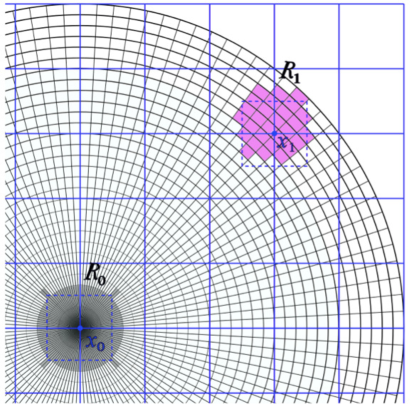
Figure 4: Remapping the points in polar coordinates to points in the grid.

Geo-indistinguishability of the discretized mechanism

We now analyze the privacy guarantees provided by our discretized mechanism. We show that the discretization preserves geo-indistinguishability, at the price of a degradation of the privacy parameter $\epsilon$.

For the sake of generality we do not require the step units along the two dimensions of $\mathcal{G}$ to be equal. We will call them grid units, and will denote by $u$ and $v$ the smaller and the larger unit, respectively. We recall that $\delta_{\theta}$ and $\delta_{r}$ denote the precision of the machine in representing $\theta$ and $r$, respectively. We assume that $\delta_{r}\leq r_{\max}\delta_{\theta}$. The following theorem states the geo-indistinguishability guarantees provided by our mechanism: $K_{\epsilon^{\prime}}$ satisfies $\epsilon$-geo-indistinguishability, within a range $r_{\max}$, provided that $\epsilon^{\prime}$ is chosen in a suitable way that depends on $\epsilon$, on the length of the step units of $\mathcal{G}$, and on the precision of the machine.

Theorem 4.1

Assume $r_{\max}<\nicefrac{{u}}{{\delta_{\theta}}}$, and let $q=\nicefrac{{u}}{{r_{\max}\delta_{\theta}}}$. Let $\epsilon,\epsilon^{\prime}\in\mathbb{R}^{+}$ such that

$$\epsilon^{\prime}+\frac{1}{u}\ln\,\frac{q+2\,e^{\epsilon^{\prime}u}}{q-2\,e^{\epsilon^{\prime}u}}\leq\epsilon$$

Then ${K}_{\epsilon^{\prime}}$ provides $\epsilon$-geo-indistinguishability within the range of $r_{\max}$. Namely, if $d({x}_{0},{x}),d({x}^{\prime}_{0},{x})\leq r_{\max}$ then:

$${K}_{\epsilon^{\prime}}({x}_{0})({x})\leq e^{\epsilon\,d({x}_{0},{x}_{0}^{\prime})}{{K}_{\epsilon^{\prime}}({x}_{0}^{\prime})({x})}.$$

The difference between $\epsilon^{\prime}$ and $\epsilon$ represents the additional noise needed to compensate the effect of discretization. Note that $r_{\max}$, which determines the area in which $\epsilon$-geo-indistinguishability is guaranteed, must be chosen in such a way that $q>2\,e^{\epsilon^{\prime}u}$. Furthermore there is a trade-off between $\epsilon^{\prime}$ and $r_{\max}$: If we want $\epsilon^{\prime}$ to be close to $\epsilon$ then we need $q$ to be large. Depending on the precision, this may or may not imply a serious limit on $r_{\max}$. Vice versa, if we want $r_{\max}$ to be large then, depending on the precision, $\epsilon^{\prime}$ may need to be significantly smaller than $\epsilon$, and furthermore we may have a constraint on the minimum possible value for $\epsilon$, which means that we may not have the possibility of achieving an arbitrary level of geo-indistinguishability.

Figure 5 shows how the additional noise varies depending on the precision of the machine. In this figure, $r_{\max}$ is set to be $10^{2}$ km, and we consider the cases of double precision ($16$ significant digits, i.e., $\delta_{\theta}=10^{-16}$), single precision ($7$ significant digits), and an intermediate precision of $9$ significant digits. Note that with double precision the additional noise is negligible.

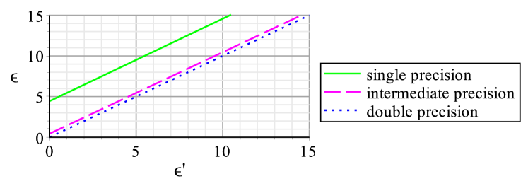
Figure 5: The relation between $\epsilon$ and $\epsilon^{\prime}$ for $r_{\max}=10^{2}$ km.

Note that in Theorem 4.1 the restriction about $r_{\max}$ is crucial. Namely, $\epsilon$-geo-indistinguishability does not hold for arbitrary distances for any finite $\epsilon$. Intuitively, this is because the step units of $\cal W$ (see Figure 4) become larger with the distance $r$ from ${x}_{0}$. The step units of $\mathcal{G}$, on the other hand, remain the same. When the steps in $\cal W$ become larger than those of $\mathcal{G}$, some ${x}$’s have an empty $\mathit{R}_{\cal W}({x})$. Therefore when ${x}$ is far away from ${x}_{0}$ its probability may or may not be $0$, depending on the position of $x_{0}$ in $\mathcal{G}$, which means that geo-indistinguishability cannot be satisfied.

4.3 Truncation

The Laplace mechanisms described in the previous sections have the potential to generate points everywhere in the plane, which causes several issues: first, digital applications have finite memory, hence these mechanisms are not implementable. Second, the discretized mechanism of Section 4.2 satisfies geo-indistinguishability only within a certain range, not on the full plane. Finally, in practical applications we are anyway interested in locations within a finite region (the earth itself is finite), hence it is desirable that the reported location lies within that region. For the above reasons, we propose a truncated variant of the discretized mechanism which generates points only within a specified region and fully satisfies geo-indistinguishability. The full mechanism (with discretization and truncation) is referred to as “Planar Laplace mechanism” and denoted by $\mathit{PL}_{\epsilon}$.

We assume a finite set $\mathcal{A}\subset\mathbb{R}^{2}$ of admissible locations, with diameter $\operatorname{diam}({\mathcal{A}})$ (maximum distance between points in $\mathcal{A}$). This set is fixed, i.e. it does not depend on the actual location $x_{0}$. Our truncated mechanism $\mathit{PL}_{\epsilon}:\mathcal{A}\to\mathcal{P}(\mathcal{A}\cap\mathcal{G})$ works like the discretized Laplacian of the previous section, with the difference that the point generated in step (a) is remapped to the closest point in $\mathcal{A}\cap\mathcal{G}$. The complete mechanism is shown in Figure 6; note that step 1 assumes that $\operatorname{diam}(\mathcal{A})<\nicefrac{{u}}{{\delta_{\theta}}}$, otherwise no such $\epsilon^{\prime}$ exists.

Theorem 4.2

$\mathit{PL}_{\epsilon}$ satisfies $\epsilon$-geo-indistinguishability.

5 Enhancing LBSs with Privacy

In this section we present a case study of our privacy mechanism in the context of LBSs. We assume a simple client-server architecture where users communicate via a trusted mobile application (the client – typically installed in a smart-phone) with an unknown/untrusted LBS provider (the server – typically running on the cloud). Hence, in contrast to other solutions proposed in the literature, our approach does not rely on trusted third-party servers.

Input: $x$	// point to sanitize
$\epsilon$	// privacy parameter
$u$, $v$, $\delta_{\theta}$, $\delta_{r}$	// precision parameters
$\mathcal{A}$	// acceptable locations
Output: Sanitized version $z$ of input $x$
1.   $\epsilon^{\prime}\leftarrow$ max $\epsilon^{\prime}$ satisfying Thm 4.1 for $r_{\max}=\operatorname{diam}(\mathcal{A})$
2.   draw $\theta$ unif. in $[0,2\pi)$	// draw angle
3.   draw $p$ unif. in $[0,1)$, set $r\leftarrow C_{\epsilon^{\prime}}^{-1}(p)$	// draw radius
4.   $z\leftarrow x+\langle r\cos(\theta),r\sin(\theta)\rangle$	// to cartesian, add vectors
5.   $z\leftarrow\operatorname{closest}(z,{\cal A})$	// truncation
6.   return $z$

Figure 6: The Planar Laplace mechanism $\mathit{PL}_{\epsilon}$

In the following we distinguish between mildly-location-sensitive and highly-location-sensitive LBS applications. The former category corresponds to LBS applications offering a service that does not heavily rely on the precision of the location information provided by the user. Examples of such applications are weather forecast applications and LBS applications for retrieval of certain kind of POI (like gas stations). Enhancing this kind of LBSs with geo-indistinguishability is relatively straightforward as it only requires to obfuscate the user’s location using the Planar Laplace mechanism (Figure 6).

Our running example lies within the second category: For the user sitting at Café Les Deux Magots, information about restaurants nearby Champs Élysées is considerably less valuable than information about restaurants around his location. Enhancing highly-location-sensitive LBSs with privacy guarantees is more challenging. Our approach consists on implementing the following three steps:

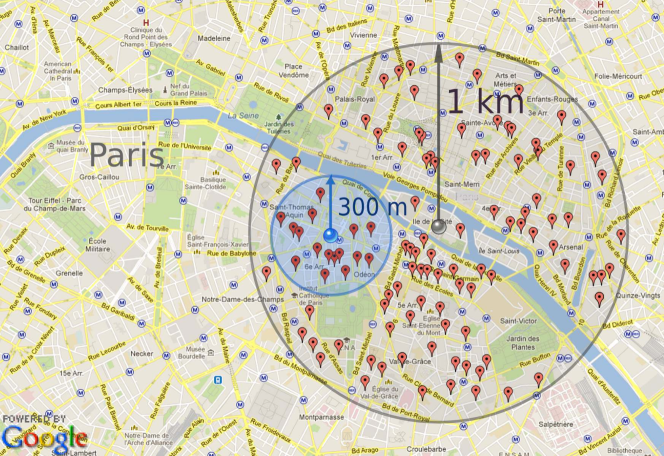
Figure 7: AOI and AOR of $\mathbf{300}$ m and $\mathbf{1}$ km radius respectively.

1. Implement the Planar Laplace mechanism (Figure 6) on the client application in order to report to the LBS server the user’s obfuscated location $z$ rather than his real location $x$.

2. Due to the fact that the information retrieved from the server is about POI nearby $z$, the area of POI information retrieval should be increased. In this way, if the user wishes to obtain information about POI within, say, $300$ m of $x$, the client application should request information about POI within, say, $1$ km of $z$. Figure 7 illustrates this situation. We will refer to the blue circle as area of interest (AOI) and to the grey circle as area of retrieval (AOR).

3. Finally, the client application should filter the retrieved POI information (depicted by the pins within the area of retrieval in Figure 7) in order to provide to the user with the desired information (depicted by pins within the user’s area of interest in Figure 7).

Ideally, the AOI should always be fully contained in the AOR. Unfortunately, due to the probabilistic nature of our perturbation mechanism, this condition cannot be guaranteed (note that the AOR is centered on a randomly generated location that can be arbitrarily distant from the real location). It is also worth noting that the client application cannot dynamically adjust the radius of the AOR in order to ensure that it always contains the AOI as this approach would completely jeopardize the privacy guarantees: on the one hand, the size of the AOR would leak information about the user’s real location and, on the other hand, the LBS provider would know with certainty that the user is located within the retrieval area. Thus, in order to provide geo-indistinguishability, the AOR has to be defined independently from the randomly generated location.

Since we cannot guarantee that the AOI is fully contained in the AOR, we introduce the notion of accuracy, which measures the probability of such event. In the following, we will refer to an LBS application in abstract terms, as characterized by a location perturbation mechanism $K$ and a fixed AOR radius. We use $\mathit{rad}_{R}$ and $\mathit{rad}_{I}$ to denote the radius of the AOR and the AOI, respectively, and $\mathcal{B}(x,r)$ to denote the circle with center $x$ and radius $r$.

5.1 On the accuracy of LBSs

Intuitively, an LBS application is $(c,rad_{I})$-accurate if the probability of the AOI to be fully contained in the AOR is bounded from below by a confidence factor $c$. Formally:

Definition 5.1 (LBS application accuracy)

An LBS application $(K,\mathit{rad}_{R})$ is $(c,\mathit{rad}_{I})$-accurate iff for all locations $x$ we have that $\mathcal{B}(x,\mathit{rad}_{I})$ is fully contained in $\mathcal{B}(K(x),\mathit{rad}_{R})$ with probability at least $c$.

Given a privacy parameter $\epsilon$ and accuracy parameters ($c,\mathit{rad}_{I}$), our goal is to obtain an LBS application ($K,\mathit{rad}_{R}$) satisfying both $\epsilon$-geo-indistinguishability and ($c,\mathit{rad}_{I}$)-accuracy. As a perturbation mechanism, we use the Planar Laplace $\mathit{PL}_{\epsilon}$ (Figure 6), which satisfies $\epsilon$-geo-indistinguishability. As for $\mathit{rad}_{R}$, we aim at finding the minimum value validating the accuracy condition. Finding such minimum value is crucial to minimize the bandwidth overhead inherent to our proposal. In the following we will investigate how to achieve this goal by statically defining $\mathit{rad}_{R}$ as a function of the mechanism and the accuracy parameters $c$ and $\mathit{rad}_{I}$.

For our purpose, it will be convenient to use the notion of ($\alpha$, $\delta$)-usefulness, which was introduced in [7]. A location perturbation mechanism $K$ is ($\alpha$, $\delta$)-useful if for every location $x$ the reported location $z=K(x)$ satisfies $d(x,z)\leq\alpha$ with probability at least $\delta$. In the case of the Planar Laplace, it is easy to see that, by definition, the $\alpha$ and $\delta$ values which express its usefulness are related by $C_{\epsilon}$ , the cdf of the Gamma distribution:

Observation 5.1

For any $\alpha>0$, $\mathit{PL}_{\epsilon}$ is ($\alpha$, $\delta$)-useful if $\alpha\leq C^{-1}_{\epsilon}(\delta)$.

Figure 8 illustrates the ($\alpha$, $\delta$)-usefulness of $\mathit{PL}_{\epsilon}$ for $r\!=\!0.2$ (as in our running example) and various values of $\ell$ (recall that $\ell=\epsilon\,r$). It follows from the figure that a mechanism providing the privacy guarantees specified in our running example ($\epsilon$-geo-indistinguishability, with $\ell\!=\!\ln(4)$ and $r\!=\!0.2$) generates an approximate location $z$ falling within $1$ km of the user’s location $x$ with probability $0.992$, falling within $690$ meters with probability $0.95$, falling within $560$ meters with probability $0.9$, and falling within $390$ meters with probability $0.75$.

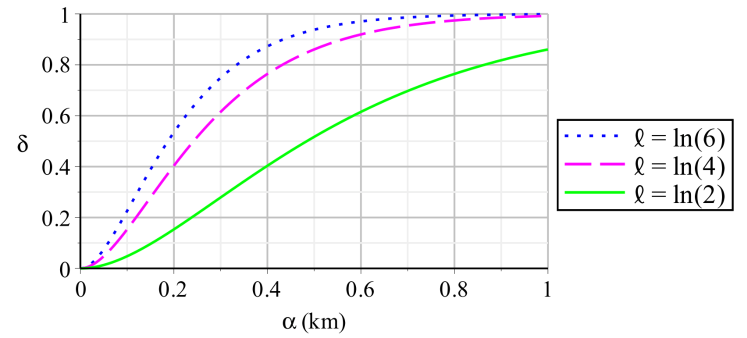
Figure 8: $(\alpha,\delta)$-usefulness for $r=0.2$ and various values of $\ell$.

We now have all the necessary ingredients to determine the desired $\mathit{rad}_{R}$: By definition of usefulness, if $\mathit{PL}_{\epsilon}$ is ($\alpha$, $\delta$)-useful then the LBS application $(\mathit{PL}_{\epsilon},\mathit{rad}_{R})$ is $(\delta,\mathit{rad}_{I})$-accurate if $\alpha\leq\mathit{rad}_{R}-\mathit{rad}_{I}$. The converse also holds if $\delta$ is maximal. By Observation 5.1, we then have:

Proposition 5.2

The LBS application $(\mathit{PL}_{\epsilon},\mathit{rad}_{R})$ is $(c$, $\mathit{rad}_{I})$-accurate if $\mathit{rad}_{R}\geq\mathit{rad}_{I}+C_{\epsilon}^{-1}(c)$.

Therefore, it is sufficient to set $\mathit{rad}_{R}=\mathit{rad}_{I}+C_{\epsilon}^{-1}(c)$.

Coming back to our running example ($\epsilon=\ln(4)/0.2$ and $\mathit{rad}_{I}=0.3$), taking a confidence factor $c$ of, say, $0.95$, leads to a $(0.69,0.95)$-useful mechanism (because $C_{\epsilon}^{-1}(c)=0.69$). Thus, $(\mathit{PL}_{\epsilon},0.99)$ is both $\nicefrac{{\ln(4)}}{{0.2}}$-geo-indistinguishable and ($0.95,0.3$)-accurate.

5.2 Bandwidth overhead analysis

As expressed by Proposition 5.2, in order to implement an LBS application enhanced with geo-indistinguishability and accuracy it suffices to use the Planar Laplace mechanism and retrieve POIs for an enlarged radius $\mathit{rad}_{R}$. For each query made from a location $x$, the application needs to (i) obtain $z=\mathit{PL}_{\epsilon}(x)$, (ii) retrieve POIs for AOR $=\mathcal{B}(z,\mathit{rad}_{R})$, and (iii) filter the results from AOR to AOI (as explained in step 3 above). Such implementation is straightforward and computationally efficient for modern smart-phone devices. In addition, it provides great flexibility to application developer and/or users to specify their desired/allowed level of privacy and accuracy. This, however, comes at a cost: bandwidth overhead.

In the following we turn our attention to investigating the bandwidth overhead yielded by our approach. We will do so in two steps: first we investigate how the AOR size increases for different privacy and LBS-specific parameters, and then we investigate how such increase translates into bandwidth overhead.

Figure 9 depicts the overhead of the AOR versus the AOI (represented as their ratio) when varying the level of confidence ($c$) and privacy ($\ell$) and for fixed values $\mathit{rad}_{I}=0.3$ and $r=0.2$. The overhead increases slowly for levels of confidence up to $0.95$ (regardless of the level of privacy) and increases sharply thereafter, yielding to a worst case scenario of a about $50$ times increase for the combination of highest privacy ($\ell=\log(2)$) and highest confidence ($c=0.99$).

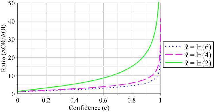
Figure 9: AOR vs AOI ratio for various levels of privacy and accuracy (using fixed $r=0.2$ and $rad_{I}=0.3$).

In order to understand how the AOR increase translates into bandwidth overhead, we now investigate the density (in km²) and size (in KB) of POIs by means of the Google Places API [2]. This API allows to retrieve POIs’ information for a specific location, radius around the location, and POI’s type (among many other optional parameters). For instance, the HTTPS request:

ΨΨhttps://maps.googleapis.com/maps/api/place/nearby
ΨΨΨsearch/json?location=48.85412,2.33316 &
ΨΨΨradius=300 & types=restaurant & key=myKey
Ψ

returns information (in JSON format) including location, address, name, rating, and opening times for all restaurants up to $300$ meters from the location ($48.85412$, $2.33316$) – which corresponds to the coordinates of Café Les Deux Magots in Paris.

We have used the APIs nearbysearch and radarsearch to calculate the average number of POIs per km² and the average size of POIs’ information (in KB) respectively. We have considered two queries: restaurants in Paris, and restaurants in Buenos Aires. Our results show that there is an average of $137$ restaurants per km² in Paris and $22$ in Buenos Aires, while the average size per POI is $0.84$ KB.

Combining this information with the AOR overhead depicted in Figure 9, we can derive the average bandwidth overhead for each query and various combinations of privacy and accuracy levels. For example, using the parameter combination of our running example (privacy level $\epsilon=\log(4)/0.2$, and accuracy level $c=0.95,\mathit{rad}_{I}=0.3$) we have a $10.7$ ratio for an average of $38$ ($\backsimeq(137/1000^{2})\times(300^{2}\times\pi)$) restaurants in the AOI. Thus the estimated bandwidth overhead is $39\times(10.7-1)\times 0.84$KB $\backsimeq 318$ KB.

Table 1 shows the bandwidth overhead for restaurants in Paris and Buenos Aires for the various combinations of privacy and accuracy levels. Looking at the worst case scenario, from a bandwidth overhead perspective, our combination of highest levels of privacy and accuracy (taking $\ell=\log(2)$ and $c=0.99$) with the query for restaurants in Paris (which yields to a large number of POIs – significantly larger than average) results in a significant bandwidth overhead (up to $1.7$MB). Such overhead reduces sharply when decreasing the level of privacy (e.g., from $1.7$ MB to $557$ KB when using $\ell=\log(4)$ instead of $\ell=\log(2)$). For more standard queries yielding a lower number of POIs, in contrast, even the combination of highest privacy and accuracy levels results in a relatively insignificant bandwidth overhead.

Restaurants		Accuracy
in Paris		$\mathit{rad}_{I}=0.3$
		$c=0.9$	$c=0.95$	$c=0.99$
Privacy	$\ell\!=\!\log(6)$	$162$ KB	$216$ KB	$359$ KB
$r\!=\!0.2$	$\ell\!=\!\log(4)$	$235$ KB	$318$ KB	$539$ KB
	$\ell\!=\!\log(2)$	$698$ KB	$974$ KB	$1.7$ MB

Restaurants		Accuracy
in Buenos Aires		$\mathit{rad}_{I}=0.3$
		$c=0.9$	$c=0.95$	$c=0.99$
Privacy	$\ell\!=\!\log(6)$	$26$ KB	$34$ KB	$54$ KB
$r\!=\!0.2$	$\ell\!=\!\log(4)$	$38$ KB	$51$ KB	$86$ KB
	$\ell\!=\!\log(2)$	$112$ KB	$156$ KB	$279$ KB

Table 1: Bandwidth overhead for restaurants in Paris and in Buenos Aires for various levels of privacy and accuracy.

Concluding our bandwidth overhead analysis, we believe that the overhead necessary to enhance an LBS application with geo-indistinguishability guarantees is not prohibitive even for scenarios resulting in high bandwidth overhead (i.e., when combining very high privacy and accuracy levels with queries yielding a large number of POIs). Note that $1.7$MB is comparable to $35$ seconds of Youtube streaming or $80$ seconds of standard Facebook usage [3]. Nevertheless, for cases in which minimizing bandwidth consumption is paramount, we believe that trading bandwidth consumption for privacy (e.g., using $\ell=\log(4)$ or even $\ell=\log(6)$) is an acceptable solution.

5.3 Further challenges: using an LBS multiple times

As discussed in Section 3.3, geo-indistinguishability can be naturally extended to multiple locations. In short, the idea of being $\ell$-private within $r$ remains the same but for all locations simultaneously. In this way the locations, say, $x_{1}$, $x_{2}$ of a user employing the LBS twice remain indistinguishable from all pair of locations at (point-wise) distance at most $r$ (i.e., from all pairs $x_{1}^{\prime}$, $x_{2}^{\prime}$ such that $d(x_{1},x^{\prime}_{1})\leq r$ and $d(x_{2},x^{\prime}_{2})\leq r$).

A simple way of obtaining geo-indistinguishability guarantees when performing multiple queries is to employ our technique for protecting single locations to independently generate approximate locations for each of the user’s locations. In this way, a user performing $n$ queries via a mechanism providing $\epsilon$-geo-indistinguishability enjoys $n\epsilon$-geo-indistinguishability (see Section 3.3).

This solution might be satisfactory when the number of queries to perform remains fairly low, but in other cases impractical, due to the privacy degradation. It is worth noting that the canonical technique for achieving standard differential privacy (based on adding noise according to the Laplace distribution) suffers of the same privacy degradation problem ($\epsilon$ increases linearly on the number of queries). Several articles in the literature focus on this problem (see [32] for instance). We believe that the principles and techniques used to deal with this problem for standard differential privacy could be adapted to our scenario (either directly or motivationally).

6 Comparison with other methods

In this section we compare the performance of our mechanism with that of other ones proposed in the literature. Of course it is not interesting to make a comparison in terms of geo-indistinguishability, since other mechanisms usually do not satisfy this property. We consider, instead, the (rather natural) Bayesian notion of privacy proposed in [36], and the trade-off with respect to the quality of service measured according to [36], and also with respect to the notion of accuracy illustrated in the previous section.

The mechanisms that we compare with ours are:

1. The obfuscation mechanism presented in [36]. This mechanism works on discrete locations, called regions, and, like ours, it reports a location (region) selected randomly according to a probability distribution that depends on the user’s location. The distributions are generated automatically by a tool which is designed to provide optimal privacy for a given quality of service and a given adversary (i.e., a given prior, representing the side knowledge of the adversary). It is important to note that in presence of a different adversary the optimality is not guaranteed. This dependency on the prior is a key difference with respect to our approach, which abstracts from the adversary’s side information.

2. A simple cloaking mechanism. In this approach, the area of interest is assumed to be partitioned in zones, whose size depends on the level of privacy we want yo achieve. The mechanism then reports the zone in which the exact location is situated. This method satisfies $k$-anonymity where $k$ is the number of locations within each zone.

In both cases we need to divide the area of interest into a finite number of regions, representing the possible locations. We consider for simplicity a grid, and, more precisely, a $9\times 9$ grid consisting of $81$ square regions of $100$ m of side length. In addition, for the cloaking method, we overlay a grid of $3\times 3=9$ zones. Figure 10 illustrates the setting: the regions are the small squares with black borders. In the cloaking method, the zones are the larger squares with blue borders. For instance, any point situated in one of the regions $1,2,3,10,11,12,19,20$ or $21$, would be reported as zone $1$. We assume that each zone is represented by the central region. Hence, in the above example, the reported region would be $11$.

Privacy and Quality of Service

As already stated, we will use the metrics for privacy and for the quality of service proposed in [36].

The first metric is called Location Privacy ($\mathit{LP}$) in [36]. The idea is to measure it in terms of the expected estimation error of a “rational” Bayesian adversary. The adversary is assumed to have some side knowledge, expressed in terms of a probability distribution on the regions, which represents the a priori probability that the user’s location is situated in that region. The adversary tries to make the best use of such prior information, and combines it with the information provided by the mechanism (the reported region), so to guess a location (remapped region) which is as close as possible to the one where the user really is. More precisely, the goal is to infer a region that, in average, minimizes the distance from the user’s exact location.

Formally, $\mathit{LP}$ is defined as:

$$\mathit{LP}=\sum_{r,r^{\prime},\hat{r}\in R}\pi(r)K(r)(r^{\prime})h(\hat{r}|r^{\prime})d(\hat{r},r)$$

where $R$ is the set of all regions, $\pi$ is the prior distribution over the regions, $K(r)(r^{\prime})$ gives the probability that the real region $r$ is reported by the mechanism as $r^{\prime}$, $h(\hat{r}|r^{\prime})$ represents the probability that the reported region $r^{\prime}$ is remapped into $\hat{r}$, in the optimal remapping $h$, and $d$ is the distance between regions. “Optimal” here means that $h$ is chosen so to minimize the above expression, which, we recall, represents the expected distance between the user’s exact location and the location guessed by the adversary.

As for the quality of service, the idea in [36] is to quantify its opposite, the Service Quality Loss (SQL), in terms of the expected distance between the reported location and the user’s exact location. In other words, the service provider is supposed to offer a quality proportional to the accuracy of the location that he receives. Unlike the adversary, he is not expected to have any prior knowledge and he is not expected to guess a location different from the reported one. Formally:

$$\mathit{SQL}=\sum_{r,r^{\prime}\in R}\pi(r)K(r)(r^{\prime})d(r^{\prime},r)$$

where $\pi$, $K(r)(r^{\prime})$ and $d$ are as above.

It is worth noting that for the optimal mechanism in [36] SQL and LP coincide (when the mechanism is used in presence of the same adversary for which it has been designed), i.e. the adversary does not need to make any remapping.

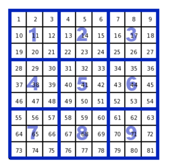
Figure 10: The division of the map into regions and zones.

Comparing the $\mathit{LP}$ for a given $\mathit{SQL}$

In order to compare the three mechanisms, we set the parameters of each mechanism in such a way that the SQL is the same for all of them, and we compare their LP. As already noted, for the optimal mechanism in [36] SQL and LP coincide, i.e. the optimal remapping is the identity, when the mechanism is used in presence of the same adversary for which it has been designed. It turns out that, when the adversary’s prior is the uniform one, SQL and LP coincide also for our mechanism and for the cloaking one.

We note that for the cloaking mechanism the SQL is fixed and it is $107.03$ m. In our experiments we fix the value of SQL to be that one for all the mechanisms. We find that in order to obtain such SQL for our mechanism we need to set $\epsilon=0.0162$ (the difference with $\epsilon^{\prime}$ in this case is negligible). The mechanism of [36] is generated by using the tool explained in the same paper.

Figure 11 illustrates the priors that we consider here: in each case, the probability distribution is accumulated in the regions in the purple area, and distributed uniformly over them. Note that it is not interesting to consider the uniform distribution over the whole map, since, as explained before, on that prior all the mechanisms under consideration give the same result.

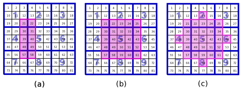
Figure 11: Priors considered for the experiments.

Figure 12 illustrates the results we obtain in terms of LP, where (a), (b) and (c) correspond to the priors in Figure 11. The optimal mechanism is considered in two instances: the one designed exactly for the prior for which it is used (“optimal-rp”, where “rp” stands for real prior), and the one designed for the uniform distribution on all the map (“optimal-unif”, which is not necessarily optimal for the priors considered here). As we can see, the Planar Laplace mechanism offers the best LP among the mechanisms which do not depend on the prior, or, as in the case of optimal-unif, are designed with a fixed prior. When the prior has a more circular symmetry the performance approaches the one of optimal-rp (the optimal mechanism).

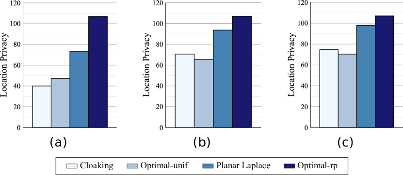
Figure 12: Location Privacy for $\boldsymbol{SQL=107.03}$ m.

Comparing the $\mathit{LP}$ for a given accuracy

The SQL metric defined above is a reasonable metric, but it does not cover all natural notions of quality of service. In particular, in the case of LBSs, an important criterion to take into account is the additional bandwidth usage. Therefore, we make now a comparison using the notion of accuracy, which, as explained in previous section, provides a good criterion to evaluate the performance in terms of bandwidth. Unfortunately we cannot compare our mechanism to the one of [36] under this criterion, because the construction of the latter is tied to the SQL. Hence, we only compare our mechanism with the cloaking one.

We recall that an LBS application $(K,\mathit{rad}_{R})$ is $(c,\mathit{rad}_{I})$-accurate if for every location $x$ the probability that the area of interest (AOI) is fully contained in the area of retrieval (AOR) is at least $c$. We need to fix $\mathit{rad}_{I}$ (the radius of the AOI), $\mathit{rad}_{R}$ (the radius of the AOR), and $c$ so that the condition of accuracy is satisfied for both methods, and then compute the respective LP measures. Let us fix $\mathit{rad}_{I}=200$ m, and let us choose a large confidence factor, say, $c=0.99$. As for $\mathit{rad}_{R}$, it will be determined by the cloaking method.

Since the cloaking mechanism is deterministic, in order for the condition to be satisfied the AOR for a given location $x$ must extend around the zone of $x$ by at least $\mathit{rad}_{I}$, In fact, $x$ could be in the border of the zone. Given that the cloaking method reports the center of the zone, and that the distance between the center and the border (which is equal to the distance between the center and any of the corners) is $\sqrt{2}\cdot 150$ m, we derive that $\mathit{rad}_{R}$ must be at least $(200+\sqrt{2}\cdot 150)$ m. Note that in the case of this method the accuracy is independent from the value of $c$. It only depends on the difference between $\mathit{rad}_{R}$ and $\mathit{rad}_{I}$, which in turns depends on the length $s$ of the side of the region: if the difference is at least $\sqrt{2}\cdot\nicefrac{{s}}{{2}}$, then the condition is satisfied (for every possible $x$) with probability $1$. Otherwise, there will be some $x$ for which the condition is not satisfied (i.e., it is satisfied with probability $0$).

In the case of our method, on the other hand, the accuracy condition depends on $c$ and on $\epsilon$. More precisely, as we have seen in previous section, the condition is satisfied if and only if $C_{\epsilon}^{-1}(c)\leq\mathit{rad}_{R}-\mathit{rad}_{I}$. Therefore, for fixed $c$, the maximum $\epsilon$ only depends on the difference between $\mathit{rad}_{R}$ and $\mathit{rad}_{I}$ and is determined by the equation $C_{\epsilon}^{-1}(c)=\mathit{rad}_{R}-\mathit{rad}_{I}$. For the above values of $\mathit{rad}_{I}$, $\mathit{rad}_{R}$, and $c$, it turns out that $\epsilon=0.016$.

We can now compare the LP of the two mechanisms with respect to the three priors above. Figure 13 illustrates the results. As we can see, our mechanism outperforms the cloaking mechanism in all the three cases.

For different values of $\mathit{rad}_{I}$ the situation does not change: as explained above, the cloaking method always forces $\mathit{rad}_{R}$ to be larger than $\mathit{rad}_{I}$ by (at least) $\sqrt{2}\cdot 150$ m, and $\epsilon$ only depends on this value. For smaller values of $c$, on the contrary, the situation changes, and becomes more favorable for our method. In fact, as argued above, the situation remains the same for the cloacking method (since its accuracy does not depend on $c$), while $\epsilon$ decreases (and consequently $\mathit{LP}$ increases) as $c$ decreases. In fact, for a fixed $r=\mathit{rad}_{R}-\mathit{rad}_{I}$, we have $\epsilon=C^{-1}_{r}(c)$. This follows from $r=C^{-1}_{\epsilon}(c)$ and from the fact that $r$ and $\epsilon$, in the expression that defines $C_{\epsilon}(r)$, are interchangeable.

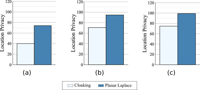
Figure 13: Location Privacy for $\mathit{rad}_{R}=(\sqrt{2}\cdot 150+200)$ m and $c=0.99$.

7 Related Work

Much of the related work has been already discussed in Section 2, here we only mention the works that were not reported there. There are excellent works and surveys [37, 26, 34] that summarize the different threats, methods, and guarantees in the context of location privacy.

LISA [9] provides location privacy by preventing an attacker from relating any particular point of interest (POI) to the user’s location. That way, the attacker cannot infer which POI the user will visit next. The privacy metric used in this work is $m$-unobservability. The method achieves $m$-unobservability if, with high probability, the attacker cannot relate the estimated location to at least $m$ different POIs in the proximity.

SpaceTwist [39] reports a fake location (called the “anchor”) and queries the geolocation system server incrementally for the nearest neighbors of this fake location until the $k$-nearest neighbors of the real location are obtained.

In a recent paper [29] it has been shown that, due to finite precision and rounding effects of floating-point operations, the standard implementations of the Laplacian mechanism result in an irregular distribution which causes the loss of the property of differential privacy. In [18] the study has been extended to the planar Laplacian, and to any kind of finite-precision semantics. The same paper proposes a solutions for the truncated version of the planar laplacian, based on a snapping meccanism, which maintains the level of privacy at the cost of introducing an additional amount of noise.

8 Conclusion and future work

In this paper we have presented a framework for achieving privacy in location-based applications, taking into account the desired level of protection as well as the side-information that the attacker might have. The core of our proposal is a new notion of privacy, that we call geo-indistinguishability, and a method, based on a bivariate version of the Laplace function, to perturbate the actual location. We have put a strong emphasis in the formal treatment of the privacy guarantees, both in giving a rigorous definition of geo-indistinguishability, and in providing a mathematical proof that our method satisfies such property. We also have shown how geo-indistinguishability relates to the popular notion of differential privacy. Finally, we have illustrated the applicability of our method on a POI-retrieval service, and we have compared it with other mechanisms in the literature, showing that it outperforms those which do not depend on the prior.

In the future we aim at extending our method to cope with more complex applications, possibly involving the sanitization of several (potentially related) locations. One important aspect to consider when generating noise on several data is the fact that their correlation may degrade the level of protection. We aim at devising techniques to control the possible loss of privacy and to allow the composability of our method.

9 Acknowledgements

This work was partially supported by the European Union 7th FP under the grant agreement no. 295261 (MEALS), by the projects ANR-11-IS02-0002 LOCALI and ANR-12-IS02-001 PACE, and by the INRIA Large Scale Initiative CAPPRIS. The work of Miguel E. Andrés was supported by a QUALCOMM grant. The work of Nicolás E. Bordenabe was partially funded by the French Defense Procurement Agency (DGA) by a PhD grant.

In this appendix we provide the technical details that have been omitted from the main body of the paper.

See 4.1

Proof .1.

The case in which ${x}_{0}={x}^{\prime}_{0}$ is trivial. We consider therefore only the case in which ${x}_{0}\neq{x}^{\prime}_{0}$. Note that in this case $d({x}_{0},{x}^{\prime}_{0})\geq u$. We proceed by determining an upper bound on ${K}_{\epsilon^{\prime}}({x}_{0})({x})$ and a lover bound on ${K}_{\epsilon^{\prime}}({x}^{\prime}_{0})({x})$ for generic ${x}_{0}$, ${x}^{\prime}_{0}$ and ${x}$ such that $d({x}_{0},{x}),d({x}^{\prime}_{0},{x})\leq r_{\max}$. Let $S$ be the set of points for which $x$ is the closest point in $\mathcal{G}$, namely:

$$S=R({x})=\{{y}\in\mathbb{R}^{2}\,|\,\forall{x}^{\prime}\in{\cal G}.\;d({y},{x}^{\prime})\leq d({y},{x}^{\prime})\}$$

Ideally, the points remapped in ${x}$ would be exactly those in $S$. However, due to the finite precision of the machine, the points actually remapped in ${x}$ are those of $R_{\cal W}({x})$ (see Section 4.2). Hence the probability of ${x}$ is that of $S$ plus or minus the small rectangles $W$ of size $\delta_{r}\times r\,\delta_{\theta}$ at the border of $S$, where $r=d({x}_{0},{x})$, see Figure 14.

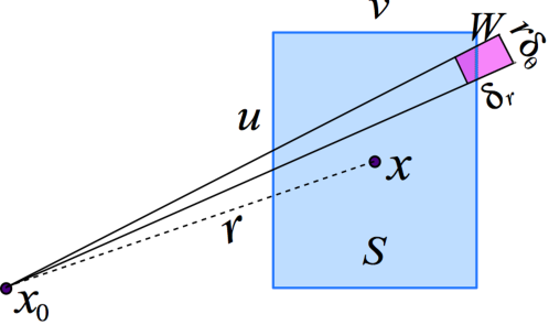
Figure 14: Bounding the probability of ${x}$ in the discrete Laplacian.

Let us denote by $S_{W}$ the total area of these small rectangles $W$ on one of the sides of $S$. Since $d({x}_{0},{x})\leq r_{\max}<\nicefrac{{u}}{{\delta_{\theta}}}$, and $\delta_{r}<r_{\max}\delta_{\theta}$, we have that $S_{W}$ is less than $\nicefrac{{1}}{{q}}$ of the area of $S$, where $q=\nicefrac{{u}}{{r_{\max}\delta_{\theta}}}$. The probability density on this area differs at most by a factor $e^{\epsilon^{\prime}u}$ from that of the other points in $S$. Finally, note that on two sides of $S$ the rectangles $W$ contribute positively to ${K}_{\epsilon^{\prime}}({x}_{0})({x})$, while on two sides they contribute negatively. Summarizing, we have:

$${K}_{\epsilon^{\prime}}({x}_{0})({x})\;\leq\;(1+\frac{2\,e^{\epsilon^{\prime}u}}{q})\int_{S}D_{\epsilon^{\prime}}({x}_{0})({x}_{1})ds$$ (3)

and

$$(1-\frac{2\,e^{\epsilon^{\prime}u}}{q})\int_{S}D_{\epsilon^{\prime}}({x}^{\prime}_{0})({x}_{1})ds\;\leq\;{K}_{\epsilon^{\prime}}({x}^{\prime}_{0})({x})$$ (4)

Observe now that

$$\frac{D_{\epsilon^{\prime}}({x}_{0})({x}_{1})}{D_{\epsilon^{\prime}}({x}^{\prime}_{0})({x}_{1})}=e^{-{\epsilon^{\prime}}(d({x}_{0},{x}_{1})-d({x}^{\prime}_{0},{x}_{1}))}$$

By triangular inequality we obtain

$$D_{\epsilon^{\prime}}({x}_{0})({x}_{1})\leq e^{\epsilon^{\prime}\,d({x}_{0},{x}^{\prime}_{0})}{D_{\epsilon^{\prime}}({x}^{\prime}_{0})({x}_{1})}$$

from which we derive

$$\int_{S}D_{\epsilon^{\prime}}({x}_{0})({x}_{1})ds\leq e^{\epsilon^{\prime}\,d({x}_{0},{x}^{\prime}_{0})}\int_{S}{D_{\epsilon^{\prime}}({x}^{\prime}_{0})({x}_{1})}ds$$ (5)

from which, using (3), (5), and (4), we obtain

$${K}_{\epsilon^{\prime}}({x}_{0})({x})\leq e^{\epsilon^{\prime}\,d({x}_{0},{x}^{\prime}_{0})}\,{K}_{\epsilon^{\prime}}({x}^{\prime}_{0})({x})\,\frac{q+2\,e^{\epsilon^{\prime}u}}{q-2\,e^{\epsilon^{\prime}u}}$$ (6)

Assume now that

$$\epsilon^{\prime}+\frac{1}{u}\ln\,\frac{q+2\,e^{\epsilon^{\prime}u}}{q-2\,e^{\epsilon^{\prime}u}}\leq\epsilon$$

Since we are assuming $d({x}_{0},{x}^{\prime}_{0})\geq u$, we derive:

$$e^{\epsilon^{\prime}\,d({x}_{0},{x}^{\prime}_{0})}\,\frac{q+2\,e^{\epsilon^{\prime}u}}{q-2\,e^{\epsilon^{\prime}u}}\leq e^{\epsilon\,d({x}_{0},{x}^{\prime}_{0})}$$ (7)

Finally, from (6) and (7), we conclude.

See 4.2

Proof .2.

The proof proceeds like the one for Theorem 4.1, except when $R({x})$ is on the border of $\mathcal{A}$. In this latter case, the probability on ${x}$ is given not only by the probability on $R({x})$ (plus or minus the small rectangles $W$ – see the proof of Theorem 4.1), but also by the probability of the part $C$ of the cone determined by ${o}$, $R({x})$, and lying outside $\mathcal{A}$ (see Figure 15).

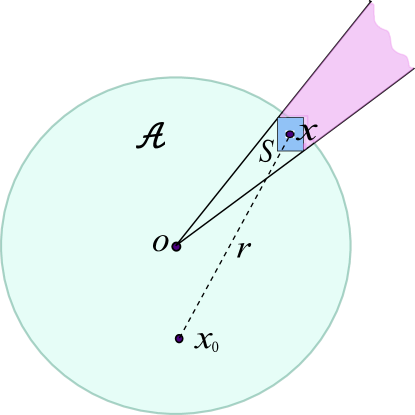
Figure 15: Probability of ${x}$ in the truncated discrete laplacian.

Following a similar reasoning as in the proof of Theorem 4.1 we get

$${K}^{T}_{\epsilon^{\prime}}({x}_{0})({x})\;\leq\;(1+\frac{2\,e^{\epsilon^{\prime}u}}{q})\int_{S\cup C}D_{\epsilon^{\prime}}({x}_{0})({x}_{1})ds$$

and

$$(1-\frac{2\,e^{\epsilon^{\prime}u}}{q})\int_{S\cup C}D_{\epsilon^{\prime}}({x}^{\prime}_{0})({x}_{1})ds\;\leq\;{K}^{T}_{\epsilon^{\prime}}({x}^{\prime}_{0})({x})$$

The rest follows as in the proof of Theorem 4.1.

References

- [1] Pew Internet & American Life Project. http://pewinternet.org/Reports/2012/Location-based-services.aspx.
- [2] Google Places API. https://developers.google.com/places/documentation/.
- [3] Vodafone Mobile data usage Stats. http://www.vodafone.ie/internet-broadband/internet-on-your-mobile/usage/.
- [4] M. Andrés, N. Bordenabe, K. Chatzikokolakis, and C. Palamidessi. Geo-indistinguishability: Differential privacy for location-based systems. Technical report, 2012. http://arxiv.org/abs/1212.1984.
- [5] C. A. Ardagna, M. Cremonini, E. Damiani, S. D. C. di Vimercati, and P. Samarati. Location privacy protection through obfuscation-based techniques. In Proc. of DAS, volume 4602 of LNCS, pages 47–60. Springer, 2007.
- [6] B. Bamba, L. Liu, P. Pesti, and T. Wang. Supporting anonymous location queries in mobile environments with privacygrid. In Proc. of WWW, pages 237–246. ACM, 2008.
- [7] A. Blum, K. Ligett, and A. Roth. A learning theory approach to non-interactive database privacy. In Proc. of STOC, pages 609–618. ACM, 2008.
- [8] K. Chatzikokolakis, M. E. Andrés, N. E. Bordenabe, and C. Palamidessi. Broadening the scope of Differential Privacy using metrics. In Proc. of PETS, volume 7981 of LNCS, pages 82–102. Springer, 2013.
- [9] Z. Chen. Energy-efficient Information Collection and Dissemination in Wireless Sensor Networks. PhD thesis, University of Michigan, 2009.
- [10] R. Cheng, Y. Zhang, E. Bertino, and S. Prabhakar. Preserving user location privacy in mobile data management infrastructures. In Proceedings of the 6th Int. Workshop on Privacy Enhancing Technologies, volume 4258 of LNCS, pages 393–412. Springer, 2006.
- [11] R. Dewri. Local differential perturbations: Location privacy under approximate knowledge attackers. IEEE Trans. on Mobile Computing, 99(PrePrints):1, 2012.
- [12] J. E. Dobson and P. F. Fisher. Geoslavery. Technology and Society Magazine, IEEE, 22(1):47–52, 2003.
- [13] M. Duckham and L. Kulik. A formal model of obfuscation and negotiation for location privacy. In Proc. of PERVASIVE, volume 3468 of LNCS, pages 152–170. Springer, 2005.
- [14] C. Dwork. Differential privacy. In Proc. of ICALP, volume 4052 of LNCS, pages 1–12. Springer, 2006.
- [15] C. Dwork. A firm foundation for private data analysis. Communications of the ACM, 54(1):86–96, 2011.
- [16] C. Dwork, M. Hardt, T. Pitassi, O. Reingold, and R. S. Zemel. Fairness through awareness. In Proc. of ITCS, pages 214–226. ACM, 2012.
- [17] C. Dwork, F. Mcsherry, K. Nissim, and A. Smith. Calibrating noise to sensitivity in private data analysis. In Proc. of TCC, volume 3876 of LNCS, pages 265–284. Springer, 2006.
- [18] I. Gazeau, D. Miller, and C. Palamidessi. Preserving differential privacy under finite-precision semantics. In Proc. of QAPL, volume 117 of EPTCS, pages 1–18. OPA, 2013.
- [19] B. Gedik and L. Liu. Location privacy in mobile systems: A personalized anonymization model. In Proc. of ICDCS, pages 620–629. IEEE, 2005.
- [20] G. Ghinita, P. Kalnis, A. Khoshgozaran, C. Shahabi, and K.-L. Tan. Private queries in location based services: anonymizers are not necessary. In Proc. of SIGMOD, pages 121–132. ACM, 2008.
- [21] M. Gruteser and D. Grunwald. Anonymous usage of location-based services through spatial and temporal cloaking. In Proc. of MobiSys. USENIX, 2003.
- [22] S.-S. Ho and S. Ruan. Differential privacy for location pattern mining. In Proc. of SPRINGL, pages 17–24. ACM, 2011.
- [23] B. Hoh and M. Gruteser. Protecting location privacy through path confusion. In Proc. of SecureComm, pages 194–205. IEEE, 2005.
- [24] A. Khoshgozaran and C. Shahabi. Blind evaluation of nearest neighbor queries using space transformation to preserve location privacy. In Proc. of SSTD, volume 4605 of LNCS, pages 239–257. Springer, 2007.
- [25] H. Kido, Y. Yanagisawa, and T. Satoh. Protection of location privacy using dummies for location-based services. In Proc. of ICDE Workshops, page 1248, 2005.
- [26] J. Krumm. A survey of computational location privacy. Personal and Ubiquitous Computing, 13(6):391–399, 2009.
- [27] K. Lange and J. S. Sinsheimer. Normal/independent distributions and their applications in robust regression. J. of Comp. and Graphical Statistics, 2(2):175–198, 1993.
- [28] A. Machanavajjhala, D. Kifer, J. M. Abowd, J. Gehrke, and L. Vilhuber. Privacy: Theory meets practice on the map. In Proc. of ICDE, pages 277–286. IEEE, 2008.
- [29] I. Mironov. On significance of the least significant bits for differential privacy. In Proc. of CCS, pages 650–661. ACM, 2012.
- [30] M. F. Mokbel, C.-Y. Chow, and W. G. Aref. The new casper: Query processing for location services without compromising privacy. In Proc. of VLDB, pages 763–774. ACM, 2006.
- [31] J. Reed and B. C. Pierce. Distance makes the types grow stronger: a calculus for differential privacy. In Proc. of ICFP, pages 157–168. ACM, 2010.
- [32] A. Roth and T. Roughgarden. Interactive privacy via the median mechanism. In Proc. of STOC, pages 765–774, 2010.
- [33] P. Shankar, V. Ganapathy, and L. Iftode. Privately querying location-based services with SybilQuery. In Proc. of UbiComp, pages 31–40. ACM, 2009.
- [34] K. G. Shin, X. Ju, Z. Chen, and X. Hu. Privacy protection for users of location-based services. IEEE Wireless Commun, 19(2):30–39, 2012.
- [35] R. Shokri, G. Theodorakopoulos, J.-Y. L. Boudec, and J.-P. Hubaux. Quantifying location privacy. In Proc. of S&P, pages 247–262. IEEE, 2011.
- [36] R. Shokri, G. Theodorakopoulos, C. Troncoso, J.-P. Hubaux, and J.-Y. L. Boudec. Protecting location privacy: optimal strategy against localization attacks. In Proc. of CCS, pages 617–627. ACM, 2012.
- [37] M. Terrovitis. Privacy preservation in the dissemination of location data. SIGKDD Explorations, 13(1):6–18, 2011.
- [38] M. Xue, P. Kalnis, and H. Pung. Location diversity: Enhanced privacy protection in location based services. In Proc. of LoCA, volume 5561 of LNCS, pages 70–87. Springer, 2009.
- [39] M. L. Yiu, C. S. Jensen, X. Huang, and H. Lu. Spacetwist: Managing the trade-offs among location privacy, query performance, and query accuracy in mobile services. In Proc. of ICDE, pages 366–375. IEEE, 2008.