Quenches and lattice simulators for particle creation

Abstract

In this paper we propose a framework for simulating approximate thermal particle production in condensed matter systems. The procedure we describe can be realized by means of a quantum quench of a parameter in the model.

In order to support this claim, we study quadratic fermionic systems in one and two dimensions by means of analytical and numerical techniques. In particular, we are able to show that a class of observables associated to Unruh–de Witt detectors are very relevant for this type of setup and that exhibit approximate thermalization.

I Introduction

The relative weakness of the gravitational field makes difficult any direct test of some of the phenomena that should characterize quantum field theory (QFT) in curved spacetimes, namely various instances of particle creation from the quantum vacuum. For the same reason, the regime in which quantum gravitational phenomena deviate significantly from the predictions of Einstein gravity (viewed as the effective field theory description of a full-fledged quantum gravity theory) seems to be still out of reach. Therefore simulators, i.e. models offering analogies with gravitational systems, could help us to develop concepts, methods and insights for the investigation of the relationship between quantum mechanics and the geometry of spacetime.

Since the seminal work of Unruh Unruh , who showed how four dimensional Lorentzian geometries can be simulated in hydrodynamical systems, the area of analogue models has flourished AnalogueReview , providing nowadays a rather large number of (classical and quantum) models based on condensed matter systems, which are able to simulate QFT in curved spaces. Furthermore, we have by now numerical and experimental results Weinfurtner:2008if ; Carusotto ; stimulated ; HawkingFilaments ; HorstmannLett ; HorstmannLong ; Rubino:2011zq which allow us to discuss concretely the validity of the theoretical predictions for phenomena like Hawking radiation and cosmological particle creation.

Most of the analogues are based on continuous approximations, hence applying methods of continuuum field theories. However, this is not the only possibility that we have. It has been already proposed to use lattice systems to model new interesting situations. For instance, the use of optical lattices has been advocated in HuRey1 and SchuetzSzpak1 ; SchuetzSzpak2 in order to explore regimes in which conventional continuum mean field descriptions fail or in which the quantum vacuum is explored in the strong external field limit, regimes difficult to achieve and to control in other quantum systems like BECs.

Another motivation for discrete analogues comes from the number of discrete Quantum Gravity proposals. In particular, the possibility that at a microscopic level continuum spacetime might be replaced by a completely combinatorial structure in the shape of a random graph (variously decorated with geometric data) is a widespread idea Approaches . Despite the variety of proposals, the manipulation of random graphs (or random complexes) within a reparametrization invariant framework presents difficulties which are so far not completely under control, especially if we try to obtain a quantitative explanation of the emergence of classical continuum spacetime and its dynamics.

In fact, in QGp1 ; QGp2 ; QGp3 ; QGp4 it has been proposed to address a simpler problem, that is the emergence of space alone, as the outcome of the collective dynamics a certain specific class of (quantum) Hamiltonians for (quantum) graphs: Quantum Graphity. Since in such a framework there is a preferred foliation related to the presence of a preferred notion of time (here radically different from space), the inclusion of Lorentz invariance (and of the full four dimensional diffeomorphism invariance) is problematic. Nonetheless, they represent ideal candidates to discuss in an explicit way at least some general features of the otherwise vague idea that space, time and geometry are emerging from pregeometric degrees of freedom. For such a purpose, different models have been introduced so far, with the objective of elucidating the way in which the dimensionality of the graphs is dynamically controlled, as well as the properties of the phase transition from the disordered, pregeometric phase to the ordered, geometric one QGp4 ; Conrady ; Chen . Possible cosmological effects due to their fundamental discrete structures have been considered recently in Quach .

As we shall argue in detail in the rest of the paper, these systems might still offer interesting insights as far as quantum field theory in curved spaces is concerned. In particular, we will show how these models can be used to simulate particle creation phenomena (either in a black hole-like configuration, like in BlackOnions , or in a cosmological setting) by analogy with Unruh effect, tying it to quench experiments, which are indeed the natural experimental setup.

Concretely, we will work with a Fermi–Hubbard model on a fixed lattice with an additional term in the Hamiltonian, which does not conserve the particle number. A similar model appeared already in the literature of Lieb–Robinson bounds and has been experimentally probed optlattnat .

The model which we consider has been initially derived from Quantum Graphity Hamma , as an effective description in which the graph is essentially frozen in a given configuration. The derivation is explained in Section IV in the section dedicated to Quantum Graphity. The application of our setup to quantum graphity’s trapped surfaces, for the sake of clarity, is at the very end of the paper, as in principle this setup could apply to other physical models.

The paper is organized as follows. Section II is devoted to the detailed explanation of the model and of the calculations that will be presented, in particular with respect to the notion of particle and detectors. In section III we first show the numerical results on the thermality of the detected particles, for various 2-dimensional square-shaped lattices and for the 1-dimensional ring. The latter is treated analytically in full detail. A subsection is devoted to the clarification of the results from the point of view of quantum quenches. Section IV explains the application to quantum graphity’s trapped surfaces, with emphasis on the subtle but important differences with the case of true black holes. Some final remarks conclude the paper.

II The analogy

II.1 Time independent Hamiltonians: detectors

Contrary to what could happen in a general relativistic context, in non-relativistic quantum mechanics, the notion of ground state (vacuum) and excited states (particles) is globally defined (see, e.g. , BirrellDavies ). Moreover, if we consider static configurations (i.e. time-independent Hamiltonians), any energy eigenstate is preserved by the unitary time evolution and, thus, particle creation effects cannot take place.

In order to overcome this obstacle and make radiation effects possible, it is necessary that the notion of particle that the detector measures does not correspond to the excitations of the Hamiltonian. This is not so unnatural since detectors are local objects, and therefore, there is no reason to think that they are be able to capture the precise structure of the eigenstates of the global Hamiltonian.

In particular, we need to introduce a notion of particle (with an associated momentum $k$ and energy $\epsilon(k)$) given in terms of some ladder operators $\eta_{k}$. Once the notion of particle that the detector measures is established, we can determine the momentum distribution (number of particles with momentum $k$) of the ground state of the system

$$n(k)=\langle GS|\eta_{k}^{\dagger}\eta_{k}|GS\rangle,$$ (1)

and see whether it follows a thermal distribution.

The notion of particle $\eta_{k}$, together with its associated momentum $k$ and energy $\epsilon(k)$, define a test Hamiltonian $H_{UDW}=\sum_{k}\epsilon(k)\eta_{k}^{\dagger}\eta_{k}$. The momentum distribution (1) that the detector measures is given by the overlap between the ground state of the system and the eigenstates states of the test Hamiltonian $H_{UDW}$.

II.2 Time dependent Hamiltonians: quenches

Another possibility for simulating particle creation phenomena is to consider time dependent Hamiltonians. If some parameter of the Hamiltonian changes fast enough, the adiabatic approximation breaks down and the system leaves its ground state. The populations of the excited states become non trivial and hence radiation is produced.

An example of such a process is a time dependent tunnelling amplitude between the sites of the lattice. This can be interpreted as a time dependent scale factor of the spatial geometry, giving the possibility to study, along the very same lines described for a black hole configuration, analogue cosmological particle production phenomena.

A particularly interesting case of a time dependent Hamiltonian is the quench setting. A quench experiment consists of preparing a quantum system in the ground state of a certain Hamiltonian, and, suddenly, changing the Hamiltonian such that the quantum state does not correspond to an eigenstate of the new Hamiltonian anymore. The system, then, is out of equilibrium an evolves non-trivially in time. The goal of quench experiments is to study the time evolution of systems and in particular, its possible relaxation to equilibrium.

Let us notice that the process of equilibration after a quantum quench for the whole system is, strictly speaking, never possible. This is due to the fact that the system evolves according to a unitary evolution. Nevertheless, what we mean by equilibration is the relaxation of the expectation values of a certain family of observables to constant quantities. The question whether the equilibrium state after a quench corresponds or not to a thermal state has been studied in several works calabrfag ; foinifluctdiss ; essevfag ; calabrese06 ; calabrese07 .

If the Hamiltonian is quenched to the Hamiltonian that defines the notion of particle in the detector setting $H_{UDW}$, then the momentum distribution of the system at any time after the quench is identical to the momentum distribution measured by the detector in the time independent case, and hence, both settings become equivalent. This is due to the fact that the observables $\eta_{k}^{\dagger}\eta_{k}$ commutes with the Hamiltonians considered before and after the quench.

The equivalence between the two settings suggests the use of quench experiments to simulate particle production also in the detector framework. Furthermore, the fact that the momentum distribution does not change along the evolution dictated by $\hat{H}_{UDW}$ allows to measure it at the most convenient time.

II.3 The model

The Hamiltonian we will consider in the present paper is the following Fermi–Hubbard model:

$$H(\Gamma,\lambda)=-J\sum_{i,j=1}^{N_{v}}A_{ij}^{(\Gamma)}a^{\dagger}_{i}a_{j}+\frac{\lambda}{2}\sum_{i,j=1}^{N_{v}}B_{ij}^{(\Gamma)}\left(a^{\dagger}_{i}a^{\dagger}_{j}+\textrm{h.c.}\right),$$ (2)

where $a_{i}$,$a^{\dagger}_{i}$ are annihilation/creation fermionic operators that annihilate/create a particle in the vertex $i$ of the background graph $\Gamma$. The matrices $A_{ij}^{(\Gamma)}$ and $B_{ij}^{(\Gamma)}$ are, respectively, the adjacency matrix of $\Gamma$ and its antisymmetrized form. The sum runs over all the $N_{v}$ vertices of the graph $\Gamma$. The coupling $J$ is the tunneling of the particles between two connected sites and $\lambda$ controls the strength of the Hamiltonian terms that do not conserve the number of particles.

In quantum graphity, the role of curvature in a continuous space-manifold is played by the connectivity of a dynamic graph, while the backreaction of matter on geometry, in graphity models, is controlled usually by a term in the Hamiltonian that annihilates particles and creates links of the graph, with the idea that the larger is the number of particles in a region, the larger is the effect on the connectivity of the curvature.

We derived this model as an effective description of Quantum Graphity in the limit of a very dilute matter content and a weak backreaction term between the particles and the graph (see Sec. IV). This violation of the number of particles related to the connectivity of the graph is produced in Hamiltonian (2) by the second term proportional to $\lambda$. In a more rigorous way, Hamiltonian (2) is exactly obtained from the quantum graphity Hamiltonian after freezing the evolution of the graph and assuming that this is in a superpositon state (see Sec. IV for details).

Let us mention that a similar effective model has been studied both theoretically and experimentally in the context of optical lattices optlattnat in order to give experimental evidence to the Lieb–Robinson bounds. We thus expect that the results of our paper could be potentially tested experimentally, given that the experimenter should be able to measure our observables.

II.4 Detector and notion of particle

In order to study particle creation effects, we need to specify the notion of particle (and its corresponding energy) that our detector will measure. In a continuous flat space, we can define particles as plane waves with a well defined momentum $\vec{k}$ and energy $\hbar^{2}k^{2}/(2m)$. We have to generalize this idea of particle to graphs.

The simplest graph one can consider is the discretization of the line or a ring lattice (in which we have under control irrelevant IR divergences). In the ring graph in particle, it is natural to define the annihilation operator of a particle with momentum $k$ as the discrete Fourier transform of the annihiliation operators in position $a_{j}$,

$$\eta_{k}=\frac{1}{\sqrt{L}}\sum_{j=0}^{L-1}\mathrm{e}^{\mathrm{i}2\pi jk/L}a_{j}\,,$$

with $L$ the number of sites of the ring. Notice that these are precisely the eigenmodes of the hopping Hamiltonian

$$H_{\textrm{Ring}}=-\sum_{j=0}^{L-1}(a_{j}^{\dagger}a_{j+1}+\textrm{h. c})=\sum_{k=0}^{L-1}\epsilon(k)\eta_{k}^{\dagger}\eta_{k}\,,$$

where $\epsilon(k)=-2\cos(2\pi k/L)$ gives us the energy of the mode $k$. In the continuum limit, both the wave function and the dispersion relation are recovered in their standard form.

Thus, when other lattice configurations are considered (torus, cylinder, etc.), it is natural to define particles as the eigenmodes of the hopping Hamiltonian supported on a regular graph. This hopping Hamiltonian is written as

$$\hat{H}_{UDW}=\sum_{i,j=1}^{N_{v}}A_{ij}^{(\Gamma_{0})}a_{i}^{\dagger}a_{j}=\sum_{k=1}^{N_{v}}\epsilon(k)\eta^{\dagger}_{k}\eta_{k},$$ (3)

where $A_{ij}^{(\Gamma_{0})}$ is the adjacency matrix of the regular graph $\Gamma_{0}$. The eigenmodes of $\hat{H}_{UDW}$, labelled by $k$, and with energy $\epsilon(k)$, define our notion of particle. These are created and annihilated by the operators $\eta_{k}^{\dagger}$ and $\eta_{k}$, and are the excitation the detector measures.

Let us mention that while $\Gamma_{0}$ is a regular graph, in general, the graph $\Gamma$ that defines Hamiltonian (2) does not have to, since it will have regions with a higher or a lower connectivity. Roughly speaking, we can construct $\Gamma$ by taking the flat graph $\Gamma_{0}$, and adding or removing links to/from it.

II.5 Calculation

The aim of our calculation is to probe how many particles (as the ones defined as in the previous section) will be present in the ground state of the Hamiltonian of (2). Therefore, we need to compute

$$n(k)=\langle GS|\eta^{\dagger}_{k}\eta_{k}|GS\rangle\,,$$ (4)

and check whether the ground state, with respect to this notion of particle, appears as a thermal state, i.e.  the momentum distribution (4) follows a Fermi–Dirac distribution.

In order for the computation of (4) to make sense, the Hilbert space of the full Hamiltonian and the one of the detector have to have some overlap (in terms of unitary mappings from one to the other). It is sufficient that the two different Hamiltonians are defined as operators on the same Hilbert space, i.e.  the graphs have the same number of nodes.

The Hamiltonian (2) is a standard quadratic model, hence, it can be diagonalized as

$$H=\sum_{j=0}^{L-1}\omega(j)\psi_{j}^{\dagger}\psi_{j},$$ (5)

by means of a Bogoliubov transformation of the fundamental particle operators, $a_{i}^{\dagger},a_{j}$. In turn, these are related by another Bogoliubov transformations to the operators $\eta,\eta^{\dagger}$. Then, the operators $\eta,\eta^{\dagger}$ will be connected to the $\psi,\psi^{\dagger}$ by the Bogoliubov transformation that is the composition of the Bogoliubov transformations that relate $\psi,\psi^{\dagger}$ to $a,a^{\dagger}$ and $a,a^{\dagger}$ to $\eta,\eta^{\dagger}$. It can be written formally as

$$\eta_{k}=\sum_{j=0}^{L-1}\left(\alpha_{kj}\psi_{j}+\beta_{kj}\psi^{\dagger}_{j}\right)\,,$$ (6)

where $\alpha_{kj}$ and $\beta_{kj}$ are the Bogoliubov coefficents. Particle creation effects will be clearly related to them.

Notice that in general the ground state of these fermionic models is not just the Fock vacuum of the quasiparticles (the eigenmodes of the given Hamiltonian), but it is a Fermi sphere due to the appearance of some negative energy modes in the spectrum (actually, this is the reason why we are using a Fermionic model, since a Bosonic one would lead to instabilities). This implies that the momentum distribution $n(k)$ will receive a contribution just by the very presence of real quasiparticles in the Fermi sphere.

III Analysis

In this section we present numerical and analytical results which support the claim of having particle production, at least in the sense of detectors. The key ingredient is the mismatch between the eigenspaces of the Hamiltonian governing time evolution and the eigenspaces of the Hamiltonian with which we set up the detector.

III.1 Numerical results

We study here three different lattice geometries: a cylinder, a torus, and a ring. We evaluate the populations $\langle\eta_{k}^{\dagger}\eta_{k}\rangle$ in the ground state of the eigenmodes of the Hamiltonian $\hat{H}_{UDW}$ that defines our notion of particles, that is, the Hamiltonian with $\lambda=0$. Finally, we check if the distribution of the occupations with respect to the energy is thermal.

In Fig. 1, the populations obtained in the three geometries are plotted with respect to the energy for $\lambda=0.3$. We observe that the observable is close to thermal in all cases. In particular, both for the cylinder and the torus, the energy modes as measured by a Unruh–de Witt detector are populated according to a Maxwell–Boltzmann distribution,

$$n_{MB}(k)\propto\mathrm{e}^{-\beta\epsilon(k)}\,,$$ (7)

and therefore in the plan $(\log n(k),\epsilon(k))$ we see a straight line with slope $-\beta$. For the case of a a circle, we observe a Fermi–Dirac distribution,

$$n_{FD}(k)=\frac{1}{\mathrm{e}^{\beta\epsilon(k)}+1}\,,$$ (8)

and the logarithm of the populations $\log(1/n(k)-1)$ scales linearly with $\epsilon(k)$.

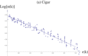
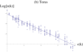
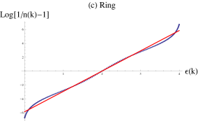
Figure 1: Functions of the number of quasiparticles $n(k)=\langle\eta_{k}^{\dagger}\eta_{k}\rangle$, evaluated numerically, in the ground state of the system with $\lambda=0.3$ for three different lattices: (a) cylinder [20x20], (b) torus [16x16] and (c) ring [300].

For different values of the parameter $\lambda$ and size of the system, we numerically evaluated the Bogoliubov transformation between the modes and their populations $n(k)$. In all cases, there are striking numerical evidences that:

• The temperature is well defined in the large lattice size limit (thermodynamic limit).

• The temperature (inverse of the slope in the plots of Fig. 1) scales proportionally to $\lambda$, i.e.

  $$T\propto\lambda\,.$$

• The higher the $\lambda$, the better is the alignment of the points on a straight line, that is, the more thermal the behavior of the radiation.

In order to better understand the thermal nature of these distributions, we solve in the next section the 1-dimensional chain with periodic boundary conditions analytically.

III.2 Analytical solution of the 1-dimensional lattice

In the one dimensional case, the Hamiltonian (2) becomes

$$H=-J\sum_{m=0}^{L-1}\left(a^{\dagger}_{m}a_{m+1}+\textrm{h. c.}\right)+\lambda\sum_{m=0}^{L-1}\left(a_{m}a_{m+1}+\textrm{H. c.}\right),$$ (9)

where $L$ is the length of lattice (chosen to be odd) and the periodic boundary conditions are imposed by the identification of $a_{0}$ with $a_{L}$. Let us point out that this Hamiltonian is equivalent to the XY model in an external magnetic field fradkin .

In order to diagonalize this model, let us exploit its translational invariance and introduce the Fourier modes

$$\eta_{k}=\frac{1}{\sqrt{L}}\sum_{m=0}^{L-1}\mathrm{e}^{-\mathrm{i}\frac{2\pi k}{L}m}a_{m}\,.$$ (10)

We note that according to this definition the mode $\eta_{-k}=\eta_{L-k}$. From now on, we will use both $[-(L-1)/2,(L-1)/2]$ and $[0,L-1]$ as the range of $k$ depending on the simplicity of the notation. In terms of these modes, the Hamiltonian (9) reads

$$H = -J\sum_{k=0}^{L-1}2\cos\left(\frac{2\pi}{L}k\right)\eta_{k}^{\dagger}\eta_{k}$$

$$+ \ \lambda\sum_{k=0}^{L-1}\left(\mathrm{e}^{-\mathrm{i}\frac{2\pi}{L}k}\eta_{k}\eta_{L-k}+h.c.\right)\,.$$

Reshuffling some terms and using the canonical anticommutation relations, the Hamiltonian can be written as

$$H=\sum_{k=0}^{L-1}2\epsilon(k)\eta_{k}^{\dagger}\eta_{k}+\mathrm{i}\sigma(k)(\eta_{k}\eta_{L-k}-\eta_{L-k}^{\dagger}\eta_{k}^{\dagger})\,,$$ (11)

where

$$\epsilon(k) =-J\cos\left(\frac{2\pi}{L}k\right)$$ (12)

$$\sigma(k) =-\lambda\sin\left(\frac{2\pi}{L}k\right)\,.$$ (13)

Let us note that while $\epsilon(k)$ is a symmetric function $\epsilon(k)=\epsilon(L-k)$, $\sigma(k)$ is anti-symmetric, $\sigma(k)=-\sigma(L-k)$.

Thus, the Hamiltonian (9) is decomposed in $(L-1)/2$ independent Hamiltonians

$$H=\sum_{k=0}^{L-1}H_{k}\,,$$ (14)

with

$$H_{k}=\epsilon(k)(\eta_{k}^{\dagger}\eta_{k}+\eta_{-k}^{\dagger}\eta_{-k})+\mathrm{i}\sigma(k)(\eta_{k}^{\dagger}\eta_{-k}^{\dagger}-\eta_{-k}\eta_{k})\,,$$ (15)

or, in matrix notation,

$$H_{k}=\left(\begin{array}[]{cc}\eta_{k}^{\dagger}&\eta_{-k}\end{array}\right)\left(\begin{array}[]{cc}\epsilon(k)&\mathrm{i}\sigma(k)\\ -\mathrm{i}\sigma(k)&-\epsilon(k)\end{array}\right)\left(\begin{array}[]{c}\eta_{k}\\ \eta_{-k}^{\dagger}\end{array}\right).$$ (16)

III.2.1 Diagonalization

First of all, let us note that

$$\left(\begin{array}[]{cc}\epsilon(k)&-\mathrm{i}\sigma(k)\\ \mathrm{i}\sigma(k)&-\epsilon(k)\end{array}\right)=\sigma(k)\sigma_{y}+\epsilon(k)\sigma_{z}\,,$$ (17)

where $\sigma_{y,z}$ are the standard Pauli matrices. In the vector space formed by the $(1,\sigma_{x},\sigma_{y},\sigma_{z})$, we have to rotate the vector $(0,0,\sigma,\epsilon)$ in order to get a vector of the form $(0,0,0,\omega)$. Hence, one immediately realizes that the diagonalizing matrix is a rotation of an angle

$$\theta(k)=\arctan\left(\frac{\sigma(k)}{\epsilon(k)}\right)\,,$$ (18)

around the X axis,

$$U=\exp\left(\mathrm{i}\frac{\theta}{2}\sigma_{x}\right)=\cos(\theta/2)\mathbb{I}+\mathrm{i}\sin(\theta/2)\sigma_{x}\,.$$ (19)

From Eqs. (16) and (19), each Hamiltonian $H_{k}$ can be diagonalized with a Bogoliubov transformation of the form:

$$\psi_{k}=\cos\left(\frac{\theta(k)}{2}\right)\eta_{k}-\mathrm{i}\sin\left(\frac{\theta(k)}{2}\right)\eta^{\dagger}_{-k}\,.$$ (20)

The Hamiltonian in terms of its eigenmodes reads

$$H=\sum_{k}\omega(k)\psi_{k}^{\dagger}\psi_{k}\,,$$ (21)

with

$$\omega_{k}=\textrm{sign}(\epsilon_{k})\sqrt{\epsilon^{2}(k)+\sigma^{2}(k)}\,.$$ (22)

The eigenvalues have then multiplicity two

$$\omega(k)=\omega(L-k)=\omega(-k)\,,$$ (23)

that is, the energy of a quasiparticle with momentum $k$ is the same as the energy a quasiparticle with momentum $-k$.

Figure 2: Dispersion relation $\epsilon(k)$ for different values of $J$ and $\lambda$; $\lambda=0$ (continuous), $|J|>|\lambda|$ (dashed), $|J|=|\lambda|$ (square function), $|\lambda|>|J|$ (points).

III.2.2 Ground state

For simplicity, we fix $J=1$ and consider $\lambda>0$ in units of $J$ by rescaling the Hamiltonian. The ground state of the system with $\lambda=0$ is a Fermi sphere, and the first excited states are gapless modes ($\epsilon(k)\propto(k-k_{F})$). In the limit of large $L$, this is a conductor. This is a direct consequence of the Goldstone theorem: the Fermi sphere ground state spontaneously breaks the global $U(1)$ symmetry of the original Hamiltonian, i.e.

$$H(a,a^{\dagger})=H(\mathrm{e}^{\mathrm{i}\alpha}a,\mathrm{e}^{-\mathrm{i}\alpha}a^{\dagger})\,.$$

However, as expected from the fact that the $\lambda$ term breaks the global $U(1)$ symmetry of the standard action, the first excited states are separated from the Fermi surface by a gap of $2\lambda$. In the limit of $L$ large, and large $\lambda$, this is an insulator. We can write then the ground state as

$$|GS\rangle=\prod_{|k|<k_{F}}\psi_{k}^{\dagger}|0\rangle_{\psi}\,,$$ (24)

where $|0\rangle_{\psi}$ is the Fock vacuum for the $\psi_{k}$ operators, and $k_{F}=(L-1)/4$ is the the radius of the Fermi sphere ($\omega(k)<0$ for $|k|<k_{F}$).

From Eq. (24), we can derive the structure of the ground state in terms of the operators $\eta_{k}$ and $\eta_{k}^{\dagger}$ (up to a global phase)

$$|GS\rangle= \prod_{k=0}^{k_{F}}(\sin(\theta(k)/2)-\mathrm{i}\cos(\theta(k)/2)\eta^{\dagger}_{k}\eta^{\dagger}_{-k})$$

$$\times\prod_{k=k_{F}+1}^{(L-1)/2}(\cos(\theta(k)/2)+\mathrm{i}\sin(\theta(k)/2)\eta^{\dagger}_{k}\eta^{\dagger}_{-k})|0\rangle_{\eta}\,,$$ (25)

and the occupation of the mode $k$ reads

$$n(k):=\langle GS|\eta_{k}^{\dagger}\eta_{k}|GS\rangle=\left\{\begin{array}[]{ll}\cos^{2}(\theta(k)/2)&\textrm{if $k\leq k_{F}$}\\ \sin^{2}(\theta(k)/2)&\textrm{if $k>k_{F}$}\end{array}\right.\,.$$

This piecewise function can be written in a more compact form by using the sine and cosine half angle formulas,

$$n(k)=\frac{1}{2}\frac{\sigma^{2}(k)}{\omega^{2}(k)+\epsilon(k)|\omega(k)|}\,.$$ (26)

Let us note that, fixed $\lambda$, the momentum distribution $n(k)$ only depends on its energy, since $\sigma$ and $\omega$ can be expressed in terms of $\epsilon$ via $\sigma^{2}=\lambda^{2}(1-\epsilon^{2})$ and $\omega^{2}=\sigma^{2}+\epsilon^{2}$.

This has a nice interpretation. Due to the presence of the Bogoliubov transformation, the Fermi sphere appears to be slightly depopulated, with the particles being radiated into the higher energy levels.

III.2.3 Analogue thermal particle production

In order to check whether the momentum distribution of the radiation measured by our detector in Eq. (26) is thermal, we have to compare it with the Fermi–Dirac distribution defined in Eq. (8).

In Fig. 3(a), the quantity $\log(n(k)^{-1}-1)$ is plotted with respect to $\epsilon(k)$ for several values of $\lambda$. If the radiation is thermal, these points should be fit by a straight line that passes through the origin an has slope $\beta$. This is precisely the behavior observed. In Fig. 3(b), the real population (continuous line) of each quasiparticle with momentum $k$ is compared to the population provided by the Fermi–Dirac distribution (dashed-line). Both distributions are very close to each other.

(a)

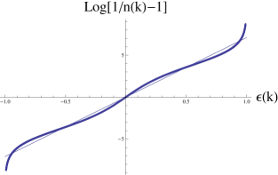
(b)

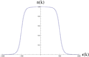
Figure 3: (a) Linear fit of the points $\left(\log(n(k)^{-1}-1),\epsilon(k)\right)$ where $n(k)$ is the momentum distribution of the modes $\eta_{k}$ in the ground state of the Hamiltonian (9) and $\epsilon(k)$ is the energy of each mode. Its alignment implies that the occupations of the modes $k$ follow a Fermi–Dirac distribution with inverse temperature corresponding to the slope. (b) Comparison between the real (continuous line) and the Fermi–Dirac (dashed line) distributions.

In order to get an analytical expression for the temperature of the radiation, let us notice that, if the distribution is a Fermi–Dirac, then

$$\beta=-4\left.\frac{\textrm{d}n}{\textrm{d}\epsilon}\right|_{\epsilon=0}\,.$$ (27)

In our case, the $n(k)$ distribution is very close to a Fermi–Dirac, and therefore, the inverse temperature given by Eq. (27) can be approximated from Eqs. (12) and (26),

$$\beta\simeq\frac{2}{\lambda},$$ (28)

matching the expectation that $T\propto\lambda$.

III.3 Comment on Thermalization

From the results of the last section we conclude that the momentum distribution of the particles that the detector would measure is very close to thermal. Let us note that, although the observables seem those of a thermal system, this does not mean that system is thermal. There are other observables (apart from the number of particles $\eta_{k}^{\dagger}\eta_{k}$ considered previously) for which the system will not look like thermal. But then, why does the momentum distribution $n(k)$ follow a thermal distribution?

In order to understand the origin of this thermal behavior, it is useful to write the state of the system in terms of the eigenbasis of the Hamiltonian. In Ref. Riera2012 , thermalization of local observables is explained by assuming a narrow energy distribution together with typicality arguments Linden2009 . In Ref. Srednicki1994 ; Rigol2008 , thermalization is a consequence of a narrow energy distribution and the Eigenstate Thermalization Hypothesis. In both cases, the temperature of the equilibrium state is determined by the position of the microcanonical energy window in the spectrum of the Hamiltonian. Determining the energy distribution of the state could explain the approximated thermalization observed by means of one of these mechanisms.

Let us write the Hamiltonian (3) that defines our notion of particle in its spectral representation for the 1-dimensional case case,

$$\hat{H}_{UDW}=\sum_{k=0}^{L-1}\epsilon(k)\eta^{\dagger}_{k}\eta_{k}=\sum_{{\bf m}\in\{0,1\}^{L}}E_{{\bf m}}|{\bf m}\rangle\!\langle{\bf m}|\,,$$ (29)

where its eigenbasis $\{|{\bf m}\rangle\}$ is the Fock basis of the $k$ modes,

$$|{\bf m}\rangle=\prod_{k=0}^{L-1}(\eta_{k}^{\dagger})^{m_{k}}|0\rangle_{\eta}\,,$$ (30)

with ${\bf m}$ the bit-string of occupations with components $m_{k}=\{0,1\}$ $\forall$ $k$. The energy $E_{{\bf m}}$ of each eigenstate $|{\bf m}\rangle$ is given by

$$E_{{\bf m}}=\sum_{k=0}^{L-1}\epsilon(k)m_{k}\,.$$ (31)

The first sum in Eq. (29) runs over the $L$ different $k$-modes, while the second one is performed over all the $2^{L}$ elements of the eigenbasis of the Hamiltonian. The state of the system in this basis becomes:

$$|GS\rangle=\sum_{{\bf m}\in\{0,1\}^{L}}c_{{\bf m}}|{\bf m}\rangle,$$ (32)

with $c_{{\bf m}}=\langle{\bf m}|GS\rangle$. These coefficents can then be derived from Eq. (III.2.2) and written as

$$c_{{\bf m}} =\mathrm{e}^{\mathrm{i}\varphi_{{\bf m}}}\prod_{k=1}^{k_{F}}\sin(\theta(k)/2)^{1-m_{k}}\cos(\theta(k)/2)^{m_{k}}\delta_{m_{k},m_{-k}}$$

$$\times\prod_{k=k_{F}+1}^{(L-1)/2}\sin(\theta(k)/2)^{m_{k}}\cos(\theta(k)/2)^{1-m_{k}}\delta_{m_{k},m_{-k}}\,\,,$$ (33)

where $\varphi_{{\bf m}}$ is a phase given by

$$\varphi_{{\bf m}}=\frac{\pi}{2}\left(3\sum_{k=1}^{k_{F}}m_{k}+\sum_{k=k_{F}+1}^{(L-1)/2}m_{k}\right)\,.$$ (34)

The Kronecker delta $\delta_{m_{k},m_{-k}}$ comes from the fact that $|GS\rangle$ is a superposition of only those Fock states with both modes $k$ and $-k$ either simultaniously occupied or empty (see Eq. (III.2.2)). This implies that only $2^{L/2}$ coefficents among the $2^{L}$ possible ones are non-trivial.

In Fig. 4, the absolute value of the coefficients of the initial state in the Hamiltonian eigenbasis given by Eq. (33) are plotted with respect to the energy. We observe that they decrease exponentially. The coefficient of the exponential decay can be numerically determined, and we have to check that for any value of $\lambda$ it coincides with $\beta/2$. The initial state can be then very well approximated by

$$|GS\rangle\simeq\sum_{{\bf m}\in M}\mathrm{e}^{\mathrm{i}\varphi_{{\bf m}}}\mathrm{e}^{-\beta/2E_{{\bf m}}}|{\bf m}\rangle\,,$$ (35)

where the sum only runs over the set of bit-strings $M$ defined by

$$M=\left\{{\bf m}\in\{0,1\}^{L}\,|\,m_{k}=m_{-k}\,\,\forall\,\,k\right\}\,.$$ (36)

Any observable $\hat{A}$ which equilibrates, will equilibrate towards its time average expected value,

$$\bar{A}=\lim_{\tau\to\infty}\frac{1}{\tau}\int_{0}^{\tau}\textrm{d}t\langle\hat{A}(t)\rangle=\textrm{Tr}(\hat{A}\omega)\,,$$ (37)

where $\omega$ is the time average state defined by

$$\omega=\lim_{\tau\to\infty}\frac{1}{\tau}\int_{0}^{\tau}\textrm{d}t\,\mathrm{e}^{-\mathrm{i}\hat{H}_{UDW}t}|GS\rangle\!\langle GS|\mathrm{e}^{\mathrm{i}\hat{H}_{UDW}t}\,.$$ (38)

Notice that $\omega$ is the apparent equilibrium state. We say “apparent” because the system is never in $\omega$, however, all those observables which equilibrate, do it towards the expected value that would be measured if the system was in $\omega$. Let us point out that in the case that the Hamiltonian has no degeneracies, $\omega$ is the completely dephased state in the Hamiltonian eigenbasis and it maximizes the von Neumann entropy given the constants of motion Gogolin2011 . Thus, the time average state $\omega$ reads in our case

$$\omega=\sum_{{\bf m}\in M}\frac{\mathrm{e}^{-\beta E_{\bf m}}}{Z_{M}}|{\bf m}\rangle\!\langle{\bf m}|\,,$$ (39)

with $Z_{M}=\sum_{{\bf m}\in M}\mathrm{e}^{-\beta E_{\bf m}}$.

Now we can understand the origin of the Fermi–Dirac distribution of the populations of each mode

$$n(k)=\textrm{Tr}(\hat{\eta}^{\dagger}_{k}\eta_{k}\omega)=\sum_{{\bf m}\in\{M|m_{k}=1\}}\frac{\mathrm{e}^{-\beta E_{\bf m}}}{Z_{M}}=\frac{1}{\mathrm{e}^{\beta\epsilon(k)}+1}\,,$$

where we have used that

$$\mathrm{e}^{-\beta E_{\bf m}}=\mathrm{e}^{-\beta\epsilon(k)m_{k}}\mathrm{e}^{-\beta\sum_{k^{\prime}\neq k}\epsilon(k^{\prime})m_{k^{\prime}}}\,.$$

Let us remark that $\omega$ in Eq. (39) is not a thermal state, since the sum does not run over all the eigenstates of the Hamiltonian, but only over those that have $m_{k}=m_{-k}$. Nevertheless, in practice, all the observables that do not contain correlations bewteen the modes $k$ and $-k$ will give the same value as if the system was in a Gibbs state.

In conclusion, we have seen that the thermal spectrum of the radiation is a consequence of the exponential decay of the energy distribution, that is, of the fact that the coefficients of the initial state written in the Hamiltonian eigenbasis decay exponentially (see Fig. 4 and Eq. (35)). This exponential decaying is not generic at all, in the sense that, most of Bogoliubov transformations relating the eigenbasis of two different Hamiltonians (even if they have the same locality structure) will not produce it. This represents another mechanism towards thermalization, where no bath is necessary and where the temperature is not given by a macroscopic energy scale (the position of the microcanonical window of energies in the spectrum) but by the intensive parameter which is quenched. It is an open question beyond the scope of this article to understand what properties two Hamiltonians have to share in order for the coefficents of an eigenstate of one Hamiltonian, spanned in the eigenbasis of the other, to decay exponentially respect to the energy.

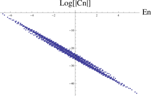
Figure 4: Coefficients of the state of the system in the Hamiltonian eigenbasis with respect to the energy in a logscale in the vertical axis. Their alignment in a straight line shows an exponential decay with the energy.

IV Application to trapping surfaces in Quantum Graphity

In this section we show how the model considered in the present paper can be derived from Quantum Graphity. Moreover, we will apply the procedure to the trapping surfaces considered previously in BlackOnions .

IV.1 Derivation

One of the most problematic features of Quantum Graphity models is their complexity. The dynamics of the graph makes the model hard to solve analytically. Thus, approximate techniques to understand the behavior of the system are required.

First of all, we briefly describe the structure of the Hubbard model on a dynamical graph introduced in Ref. QGp2 . The Hilbert space of the system is $\mathcal{H}_{\textrm{links}}\otimes\mathcal{H}_{\textrm{particles}}$ with $\mathcal{H}_{\textrm{links}}=\bigotimes_{i=1}^{N_{v}(N_{v}-1)/2}\mathbb{C}^{2}$, $\mathcal{H}_{\textrm{particles}}=\bigotimes_{i=1}^{N_{v}}\mathcal{H}_{i}$ and $\mathcal{H}_{i}$ the local Hilbert space of one site. Its Hamiltonian can be written as

$$H_{\textrm{total}}=H_{\textrm{links}}+H_{\textrm{particles}}+H_{\textrm{BR}}\,,$$ (40)

where $H_{\textrm{links}}$ describes the dynamics of the graph (space), $H_{\textrm{particles}}$ is the Hamiltonian for the particles (matter), and $H_{\textrm{BR}}$ corresponds to the backreaction interaction between space and matter. More explicitly, these Hamiltonians read

$$H_{\textrm{links}} =-U\sum_{(i,j)}\sigma^{z}_{(i,j)}\,,$$ (41)

$$H_{\textrm{particles}} =-t\sum_{(i,j)}P_{ij}\otimes(a^{\dagger}_{i}a_{j}+a_{i}a^{\dagger}_{j})\,,$$ (42)

$$H_{\textrm{BR}} =\lambda\sum_{(i,j)}\left(S^{-}_{(i,j)}\otimes a^{\dagger}_{i}a^{\dagger}_{j}+S^{+}_{(i,j)}\otimes a_{i}a_{j}\right),$$ (43)

where $P_{ij}=|1\rangle\!\langle 1|_{ij}$ is the projector onto the edge $(i,j)$, $S^{+}_{ij}=|1\rangle\langle 0|_{ij}$ and $S^{-}_{ij}=|0\rangle\langle 1|_{ij}$, and $U$, $t$, and $\lambda$ set the speed of the oscillations of the links, the tunneling rate and the backreaction strength respectivelly. Notice that in the Hamiltonian for the matter $H_{\textrm{particles}}$ the interaction among the particles has been neglected, but naturally it can be included. However, for the phenomena we are interested in, we do not really need interactions, and we can work with free fields. First of all, let us assume a situation in which matter degrees of freedom do not affect the graph, i.e. their coupling to the dynamical graph is small compared to hopping one. This means that the edges of the graph can be considered to be constant in time, and thus a fixed graph in the first approximation. However, we will still retain the quantum structure of the graph, i.e. links can be still in a superposition of on and off states. In this approximation, we can derive the Hamiltonian (2) from Quantum Graphity.

In order to see this, we consider the matrix-elements of the Hamiltonian (40) applied to a particular quantum graph, and realize that these are the same as those of the Hamiltonian in Eq. (2):

$$\langle\phi_{m}|H|\phi_{n}\rangle=\left(\langle\phi_{m}|\otimes\langle\psi_{\textrm{space}}|\right)H_{\textrm{total}}\left(|\phi_{n}\rangle\otimes|\psi_{\textrm{space}}\rangle\right)\,,$$ (44)

with the quantum state for the links fixed to

$$|\psi_{\textrm{space}}\rangle=\prod_{i,j}Q^{A_{ij}}|0\rangle^{\otimes\frac{N_{v}(N_{v}-1)}{2}}\,,$$ (45)

where $Q$ is a Hadamard gate, $Q|0\rangle=1/\sqrt{2}(|0\rangle+|1\rangle)$, and $A_{ij}$ is the adjacency matrix of the graph.

The state $|\psi_{\textrm{space}}\rangle$ is then a product state of all the links in the state $|0\rangle$ except those links that we would like to have active in the effective model, which are in the superposition

$$|+\rangle=\frac{1}{\sqrt{2}}\left(|0\rangle+|1\rangle\right)=Q|0\rangle\,.$$ (46)

In order to prove Eq. (44) it is only necessary to realize that

$$\langle+|P|+\rangle =\langle+|S^{\pm}|+\rangle=\frac{1}{2}$$ (47)

$$\langle 0|P|0\rangle =\langle 0|S^{\pm}|0\rangle=0\,.$$ (48)

We argue then that the Hamiltonian of Eq. (2) can be considered as an effective model in the case in which the graph is in a equal superposition of on and off states.

Some comments are in order. First of all, let us notice that the bosonic model is unstable in the thermodynamic limit in which the number of nodes of the graph goes to infinity. This is due to the fact that the energy can be decreased by increasing the number of bosons in the graph. Morever, the model is reliable as an effective model of Quantum Graphity as long as the number of particles $N_{p}<2L+N_{i}$, where $L$ is the number of links and $N_{i}$ is the number of particles in the states $|\psi_{\textrm{total}}\rangle=|\psi_{graph}\rangle\otimes|\psi_{part}\rangle$. The reason is that in Quantum Graphity the quantity $Q=N-2L$ is conserved.

IV.2 Unruh–de Witt detectors

In order to apply the procedure we described in the first part of the paper to Quantum Graphity, it is necessary to introduce the proper interpretation to the Unruh–de Witt observables introduced previously. We use the fact that particle states are identified by the behavior of suitably defined detectors, i.e. devices that count the number of excitations associated to the measured quantum state. As in the case of QFT in curved spaces, these detectors will be associated to an observer, and hence an Hamiltonian with respect to which states are classified. In the case of QFT in curved spaces, particle production as the Unruh effect can be purely kinematical phenomena associated to the mismatch between the notion of particle associated to different observers, possessing, effectively, different Hamiltonians. Here we consider the ideal experiment of an observer that constructs his detector in a region where the background graph is essentially regular (flat), and hence moves towards a region of high connectivity, interpreted as a black hole analogue. The readings of these detectors will be then influenced by the change in the notion of particle, ultimately associated to the structure of the graph. The calculations, then, are the same as those in the first part of the paper, although the quench involves also the structure of the graph, apart from the parameter $\lambda$.

IV.3 Difficulties with the particle production interpretation

In Hamma ; BlackOnions it has been shown that certain graphs configurations might work effectively as black holes. It has been shown that curvature is related to variations in the connectivity of the graph. A rather extreme case is when the otherwise random graph contains a highly connected region, $\mathscr{B}$, i.e. a subset of nodes which are connected by a link with almost any other node of the subset itself. In a certain limit (related to the size of $\mathscr{B}$) this region becomes a trapped region, i.e. a region from which particles cannot escape, once they enter it.

As discussed in BlackOnions , this phenomenon is rather peculiar with respect to the usual classical intuition in terms of bundles of geodesics. Indeed, it can be shown that the lower energy eigenstates correspond to the case in which the particles are trapped into this region. Moreover, the gap between the ground state and the excited states (with zero angular momentum) is proportional to the local degree (connectivity) of the graph. The size of the gap is finite for finite graphs, and hence these regions are not completely trapping. However, the larger is the size of this region (and thus the gap), the larger energy needs to be transferred to a trapped particle to kick it out of it.

We are interested in the following question: can we see Hawking radiation? Unless we use this quench formalism, this is rather unlikely.

One way to see this is to say that, while the region $\mathscr{B}$ behaves as a trapping region, it is not associated to an ergoregion where negative energy modes can be stored. A more precise statement involves the unique well defined notion of ground state and particles so far available in these models. These are limitations typical of any ordinary non-relativistic approach to this problem and as such, also Quantum Graphity suffers of it.

However, we will ask the following practical question. How will a particle detector react when lowered near the region $\mathscr{B}$? An important point to make explicit here is that the detector will work as an external apparatus, i.e. is not assumed to be built in terms of the same matter fields living on the graph. If this black hole configuration were realized in a lab, the detector we are referring to will be a scanner, a particle counter operated from the experimenter in the lab, who would just count the clicks corresponding to suitably defined notion of particle. In turn a particle is defined as an excitation above the ground state of a given Hamiltonian.

Formally, the setup described in the previous sections apply straightforwardly to the trapped surface lattice described above. For increasing values of $\lambda$, the logarithm of the population number becomes more and more a straight line with negative slope. This result is consistent with the findings in the 1-dimensional model. We thus expect that this phenomenon might be, to a certain extent, independent from the dimensionality of the lattice or from its connectivity.

We performed simulations for the lattice with cylindrical topology and with a complete graph attached to one end of the cylinder. This graph has been as a model of trapped surface in BlackOnions . We report the results here for simplicity, as we do not believe the plots have particular relevance, other than showing a particular slow convergence. The parameter $M$ which is the number of nodes in the angular coordinate of the cylinder, is also the size of the complete graph. We observe that for increasing values of $M$, the temperature obtained from the fit of the logarithm of the population number is proportional to the value of $\lambda$. There is a reason for this, which we believe is easier to understand in the effective 1-dimensional model obtained in BlackOnions . In this case, the Hamiltonian for the modes with zero angular momentum is given, for $\lambda=0$:

$$H_{\textrm{eff}}=-\sum_{i=0}^{R}J_{i}(a_{i}^{\dagger}a_{i+1}+\textrm{h. c.})$$ (49)

where $J_{0}=MJ$ and $J_{i}=J$ for $i>1$. When $M\gg 1$, the effective Hamiltonian of the model is the one with a node $0$ disconnected from the rest of the graph. In the original 2-dimensional model, this means that the complete graph can be considered as disconnected from the rest of the graph and the ground state becomes the product of the ground state for the complete region and the one for the cylindrical lattice, which then reduces the analysis to the one of the cylindrical lattice. Thus, the complete graph, as a matter of fact, does not change the temperature of observed radiation but, indeed, the more the region is trapping, the more the temperature converges to the value of the flat one. This is in fact a negative result, as it means that the radiation observed by the Unruh–de Witt detectors are not related to the trapping region, but only the quenching of the parameter $\lambda$.

V Conclusions

In this paper we investigated the possibility of using quantum quenches for simulating effects of quantum field theory in curved spacetime. This research was inspired by ideas arised in the context of Quantum Graphity models, but can be placed also in the context of analogue models.

A certain number of analogue models have been proposed in order to simulate gravitational phenomena or effects of quantum field theory in the presence of curved geometries, e.g. Hawking radiation and cosmological particle production. In our case, our proposal is different from previous models since we do not rely on the appearance of effective causal horizons, but rather on a different origin of the mismatch between notion of particles as they are defined for different detectors.

In fact, we have shown that by considering Hamiltonians which do not conserve the particle number operator we can simulate approximate thermal particle production by means of a Quantum Quench. Quantum quenches are very interesting for many reasons. First of all, for many quantum mechanical systems it was shown that many observables thermalize in the long time regime after a quantum quench. The mechanism is still poorly understood, even though it is thought that this might be related to the eigenstates thermalization hypothesis Deutsch ; Srednicki . The setting we proposed is related, as we have seen, to the quantum quench of one parameter in the Hamiltonian. We proposed to consider first the ground state of a Fermi–Hubbard model and then to perform a sudden quench of a parameter associated to a particle number non-conserving term in the Hamiltonian. We have shown analytically and numerically that the expectation value of Unruh–de Witt detectors is very close to thermal. This can be achieved by relating the quenched and unquenched Hamiltonian through a Bogoliubov transformation.

Some comments are in order. First of all, the expectation values of the number of particle in each mode do not evolve in time, thus their value just after the quench is the same they would have long after it. This situation is similar to the one appearing in the context of quantum quenches, long after the quench, with the important difference that, contrarily to time-evolving observables, these can be measured right after the quench and do not need to wait the “relaxation” of the system.

The search for thermality is a very common aspect in quench settings. While the total system is in a pure state, the expectation value of some observable are very close to thermal in the long time regime. This is confirmed by our calculations and numerical simulations, as the inspection of the occupation number of modes corresponding to particles detected in analogue detectors. This could represent a new connection between the broad area of quantum systems in the laboratory and simulators for gravity.

However, the direct application to the case of black holes, as we have argued, is not appropriate, given that the same particle creation effect is present in backgrounds that do not possess obvious causal boundaries.

Indeed, when analyzing the case of black hole-like graphs appearing in Quantum Graphity, to see whether they could be emitters of Hawking radiation, we could show that the temperature of the Planck distribution did not depend on the size of the trapped-surface, but indeed converged to a value independent from the geometrical properties of the trapped surface. We gave an explanation for this, based on the fact that the effective coupling between the trapping region and the rest of the graph decreases with the size of the trapped surface.

Nonetheless, along the lines of Weinfurtner:2008if , the setup that we described in the present paper could be used to simulate cosmological particle production, making the parameters of the Hamiltonian functions of time, controlled by the experimenter.

Aknowledgements

The authors are indebted to Alioscia Hamma for useful comments in the early stages of the work and Maurizio Fagotti for several comments. This research was supported by an NSERC and the Humboldt Foundation. Research at Perimeter Institute is supported by the Government of Canada through Industry Canada and by the Province of Ontario through the Ministry of Research & Innovation. F.C. is indebted to the University of Waterloo, the Perimeter Institute for Theoretical Physics and the Albert Einstein Institute in Potsdam for the hospitality and financial support during the period this work has been carried on.

References

- [1] W.G. Unruh. Phys.Rev.Lett., 46:1351–1353, 1981.
- [2] S. Liberati C. Barcelo and M. Visser. Living Rev.Rel., 8:12, 2005.
- [3] M. Visser S. Weinfurtner, P. Jain and C. W. Gardiner. Class.Quant.Grav., 26:065012, 2009.
- [4] S. Fagnocchi I. Carusotto and A. Fabbri A. Recati, R. Balbinot. New J.Phys., 10:103001, 2008.
- [5] S. Weinfurtner et al. Phys.Rev.Lett., 106:021302, 2011.
- [6] F. Belgiorno, S. L. Cacciatori, M. Clerici, V. Gorini, G. Ortenzi, L. Rizzi, E. Rubino, V. G. Sala, and D. Faccio. Phys. Rev. L., 105(20):203901, November 2010.
- [7] et al. B. Horstmann. Phys.Rev.Lett., 104:250403, 2010.
- [8] B. Horstmann et al. New J.Phys., 13:045008, 2011.
- [9] E. Rubino, F. Belgiorno, S.L. Cacciatori, M. Clerici, V. Gorini, et al. New J.Phys., 13:085005, 2011.
- [10] A. M. Rey, B. L. Hu, E. Calzetta, A. Roura, and C. W. Clark. Phys. Rev. A, 69(3):033610, March 2004.
- [11] N. Szpak and R. Schützhold. Phys. Rev. A, 84(5):050101, November 2011.
- [12] N. Szpak and R. Schutzhold. New J.Phys., 14:035001, 2012.
- [13] D. Oriti. Approaches to quantum gravity: Toward a new understanding of space, time and matter. Cambridge University Press, Cambridge, 2009.
- [14] F. Markopoulou T. Konopka and L. Smolin. 2006.
- [15] S. Severini T. Konopka, F. Markopoulou. Phys.Rev., D77:104029, 2008.
- [16] T. Konopka. Phys.Rev., D78:044032, 2008.
- [17] F. Caravelli and F. Markopoulou. Phys.Rev., D84:024002, 2011.
- [18] P. Horava. Phys.Rev., D79:084008, 2009.
- [19] J. Ambjorn, A. Gorlich, J. Jurkiewicz, and R. Loll. Phys.Lett., B690:420–426, 2010.
- [20] F.Conrady. J.Statist.Phys., 142:898, 2011.
- [21] S. S. Plotkin S. Chen. 2012.
- [22] A. M. Martin J. Q. Quach, C.-H. Su and A. D. Greentree. Phys. Rev. D 86, 044001, 2012.
- [23] F. Markopoulou F. Caravelli, A. Hamma and A. Riera. Phys.Rev., D85:044046, 2012.
- [24] M. Cheneau, P. Barmettler, D. Poletti, M. Endres, P. Schauß, T. Fukuhara, C. Gross, I. Bloch, C. Kollath, and S. Kuhr. Nature (London), 481:484–487, January 2012.
- [25] A. Hamma et al. Phys.Rev., D81:104032, 2010.
- [26] N.D. Birrell and P.C.W. Davies. Quantum fields in curved space. 1982.
- [27] M. Fagotti P. Calabrese, F. H. L. Essler. Phys. Rev. Lett. 106, 227203, 2011.
- [28] A. Gambassi L. Foini, L. F. Cugliandolo. Phys. Rev. B 84, 212404, 2011.
- [29] M. Fagotti F. H. L. Essler, S. Evangelisti. Phys. Rev. Lett. 109, 247206, 2012.
- [30] P. Calabrese and J. Cardy. Phys. Rev. Lett. 96, 136801, 2006.
- [31] P. Calabrese and J. Cardy. J. Stat. Mech.: Theory Exp. P06008, 2007.
- [32] E. H. Fradkin. Field theories of condensed matter systems. 1991.
- [33] C. Gogolin A. Riera and J. Eisert. Phys. Rev. Lett. 108, 080402, 2012.
- [34] A. J. Short N. Linden, S. Popescu and A. Winter. Phys. Rev. E 79, 061103, 2009.
- [35] M. Srednicki. Phys. Rev. E 50 888, 1994.
- [36] V. Dunjko M. Rigol and M. Olshanii. Nature 452 854-858, 2008.
- [37] M. P. Mueller C. Gogolin and J. Eisert. Phys. Rev. Lett. 106, 040401, 2011.
- [38] J. M. Deutsch. Phys. Rev. A 43, 2046, 1991.
- [39] M. Srednicki. J. Phys. A 32, 1163, 1999.