Interaction of Traveling Waves with Mass-With-Mass Defects within a Hertzian Chain

Abstract

We study the dynamic response of a granular chain of particles with a resonant inclusion (i.e., a particle attached to a harmonic oscillator, or a mass-with-mass defect). We focus on the response of granular chains excited by an impulse, with no static precompression. We find that the presence of the harmonic oscillator can be used to tune the transmitted and reflected energy of a mechanical pulse by adjusting the ratio between the harmonic resonator mass and the bead mass. Furthermore, we find that this system has the capability of asymptotically trapping energy, a feature that is not present in granular chains containing other types of defects. Finally, we study the limits of low and high resonator mass, and the structure of the reflected and transmitted pulses.

I Introduction

Granular crystals consisting of tightly packed arrays of solid particles, elastically deforming upon contact, present interesting dynamical features that enabled fundamental physical discoveries and suggested new engineering applications. Most studies of granular crystals focused on the highly nonlinear dynamic response of these systems  nesterenko1 ; sen08 ; nesterenko2 ; coste97 ; dar06 ; hong05 ; fernando ; doney06 ; dev08 ; dar05 ; spadoni10 ; dar05b ; ahnert ; linden ; hascoet ; job ; vakakis ; theo ; chiaradef ; chiara_nature ; theocharis_pre ; sen . One-dimensional (1D) granular crystals have been studied in a number of analytical, numerical and experimental investigations; see in sen08 for a recent review of this topic. The ability to use a wide variety of materials and bead sizes, as well as the tunability of the response within the weakly or strongly nonlinear regime makes granular crystals a natural paradigm for physical explorations of wave phenomena and the effect of nonlinearity on them nesterenko2 ; coste97 . On the engineering side, this tunability makes such crystals promising candidates for numerous applications, including shock and energy absorbing materials dar06 ; hong05 ; fernando ; doney06 , actuating and focusing devices dev08 ; spadoni10 , and sound scramblers or filters dar05 ; dar05b ; chiara_nature .

To model the dynamics of granular chains, Hertzian interparticle interactions (proportional to the relative displacement of adjacent bead centers raised to the $3/2$ power in the case of spherical beads) have been established as the canonical approach nesterenko1 . These chains have been shown to support the emergence of nonlinear traveling waves, which have been described through different types of partial differential equation models (see, e.g., ahnert ) or even by binary collision particle models (see, e.g., linden ). Although these waves are treated as compactly supported in the continuum approximations, they decay with a doubly exponential power law english ; atanas (i.e. extremely fast, but their support is not genuinely compact).

Once a chain of particles is excited by an impulse, more than 99% of its energy is rapidly and spontaneously rearranged into one or more of such nonlinear traveling waves (TW) hinch . Examining the interaction of the resulting TWs with a defect has been of particular interest from the point of view of applications (e.g. for detecting cracks dev08 or for detecting other irregularities in a medium (see e.g., sen_etal05 and references therein). A pioneering study in this regard was the computational work of hascoet , which examined both the case of a light defect and the resulting symmetric emission of traveling waves in both directions by the defect, and that of a heavy defect, which produced a train of solitary waves asymmetrically to the right of the defect. The theme of impact upon a light defect has been revisited in the work of job where the synergy of experiments, numerical computations and analytical approximations demonstrated the possibility of transient breather formation in the system. Very recently, the problem was also revisited from a chiefly analytical point of view in vakakis , where a reduction of the problem to a chain of three beads solved using a multi-scale expansion was used. This enabled an accurate capturing of the slow dynamics of the defect bead and its neighbors, along with the fast transient breathing dynamics of the light bead. It should be noted that defects have also been studied in such granular chains in the presence of a precompression force (creating an underlying linear limit and hence the potential for a weakly nonlinear regime) in the bulk, where the formation of defect breathing modes has been elaborated both analytically/numerically theo and numerically/experimentally chiaradef . The usefulness of defect breathing modes (at one edge of the chain) as generators of acoustic diode type effects has also been explored recently in chiara_nature . We also mention in passing the consideration of interactions of traveling breathers with defects in a “Newton’s cradle” model where the Hertzian chain has a local oscillator associated with each bead james1 .

In this paper, we will consider the interaction of a solitary wave with a new kind of defect, consisting of a secondary mass attached to one of the beads of the chain through a linear spring, as shown in Fig. 1. We will refer to this defect as a mass with mass (MwM) defect.

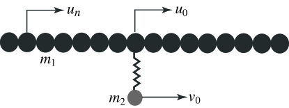
Figure 1: Diagram of a granular chain containing a mass-with-mass defect.

A MwM defect can be implemented experimentally by attaching a resonant solid structure to one of the beads, as shown in Fig. 2. Such a structure should be designed carefully to avoid higher-order normal modes of the resonant structure to participate in the dynamics of the system. A ring resonator vibrating in its piston normal mode would satisfy this requirement and is able to provide the values of spring stiffness and secondary mass needed to reproduce experimentally the effects that we have predicted theoretically.

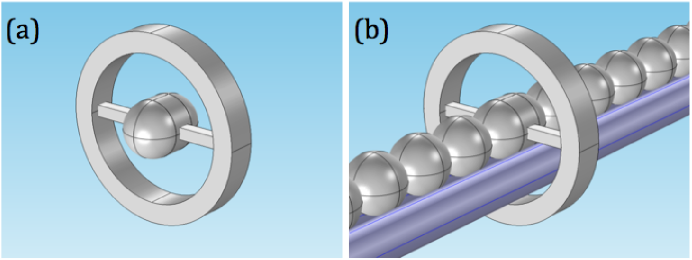
Figure 2: Suggested experimental implementation of the mass-with-mass defect. (a) Defect bead with the ring resonator that provides the mass-with-mass. (b) Part of the suggested experimental setup containing the MwM defect.

Meanwhile, the interaction of the defect bead with the neighboring particles is preserved as Hertzian. A feature of a granular chain with a MwM defect is the existence of an underlying linear oscillator at the defect. This oscillator presents the potential for long-term energy trapping, a feature that cannot be present in the mass defects considered in earlier studies. We examine various limits of the system, especially focusing on the limit of small secondary mass, which is analytically tractable and able to reproduce much of the physics of the interaction between a solitary wave and a MwM defect. We also separately consider the limit of very large secondary mass, where the reflected pulse has much larger energy, as well as the intermediate regime, where an emission of a train of transmitted solitary waves that have progressively decreasing amplitudes and speeds is observed.

Our presentation is organized as follows. In Section II, we introduce the model and the associated quantities that will be monitored. In Section III, we discuss the numerical observations of a traveling wave interacting with the MwM defect in the regimes of a small, intermediate and large secondary mass. We also briefly comment on the case of several defects. In Section IV we analyze the limit of small secondary mass using two approaches: a direct perturbation method that approximates the system in this limit as a local oscillator driven by a solitary wave and a multiscale analysis of a reduced model that captures some of the prototypical features of the full system. Section V contains the summary of our findings and the discussion of possible future directions.

II The model

We will consider a granular chain of identical spherical elastic beads of mass $m_{1}$ each. Let $u_{n}(t)$ denote the displacement of the $n$th bead from its equilibrium position and denote $\dot{u}_{n}(t)=u_{n}^{\prime}(t)$, $\ddot{u}_{n}(t)=u_{n}^{\prime\prime}(t)$. The interaction between $n$th and $(n+1)$th beads is governed by Hertz interaction potential

$$U=\dfrac{2a}{5}(u_{n}-u_{n+1})_{+}^{5/2},$$

where $(x)_{+}=x$ when $x>0$ and equals zero otherwise, and $a>0$ is a material constant. The beads thus interact only when they overlap and are not subject to a force when the overlap is absent. The defect bead, at $n=0$, is attached to another mass, $m_{2}$, via a linear spring of stiffness $K>0$, as shown in Fig. 1. This mass is constrained to move in the horizontal direction, with displacement $v_{0}(t)$. The equations of motion are:

$$\begin{split}m_{1}\ddot{u}_{n}&=a\biggl{(}(u_{n-1}-u_{n})_{+}^{3/2}-(u_{n}-u_{n+1})_{+}^{3/2}\biggr{)}-K(u_{0}-v_{0})\delta_{n0}\\ m_{2}\ddot{v}_{0}&=K(u_{0}-v_{0}),\end{split}$$ (1)

where we used the Kronecker delta, $\delta_{n0}=1$ when $n=0$ and zero otherwise. We assume that all masses, except the $j$th bead, for some $j<0$, are initially at rest, and the beads in the chain just touch their neighbors at $t=0$. The $j$th bead is excited by setting its initial velocity to $V>0$. The initial conditions are thus:

$$u_{n}(0)=v_{0}(0)=0,\qquad\dot{v}_{0}(0)=0=\dot{u}_{n}(0),\quad n\neq j,\qquad\dot{u}_{j}(0)=V,\quad j<0.$$ (2)

It is convenient to rescale (1), (2) by introducing dimensionless displacements $\bar{u}_{n}$, $\bar{v}_{0}$ and time $\bar{t}$ related to the original variables via linden

$$u_{n}=\biggl{(}\dfrac{m_{1}V^{2}}{a}\biggr{)}^{2/5}\bar{u}_{n},\quad v_{0}=\biggl{(}\dfrac{m_{1}V^{2}}{a}\biggr{)}^{2/5}\bar{v}_{0},\quad t=\dfrac{1}{V}\biggl{(}\dfrac{m_{1}V^{2}}{a}\biggr{)}^{2/5}\bar{t}.$$ (3)

The two dimensionless parameters are

$$\epsilon=\dfrac{m_{2}}{m_{1}},$$ (4)

the ratio of the two masses, and

$$\kappa=\dfrac{K}{m_{1}^{1/5}a^{4/5}V^{2/5}},$$ (5)

which measures the strength of the linear elastic spring in the mass-with-mass defect relative to the Hertzian potential stiffness at the particular $V$. In what follows, we set $\kappa=1$ for simplicity (for any $K$, we can suitably select $V$ to achieve this in Eq. (5)), while focusing on the effect of $\epsilon$. Substituting (3), (4) and $\kappa=1$ into (1) and (2) and dropping the bars on the new variables, we obtain

$$\begin{split}\ddot{u}_{n}&=(u_{n-1}-u_{n})^{3/2}_{+}-(u_{n}-u_{n+1})^{3/2}_{+}-(u_{0}-v_{0})\delta_{n0}\\ \epsilon\ddot{v}_{0}&=u_{0}-v_{0}\end{split}$$ (6)

and

$$u_{n}(0)=v_{0}(0)=0,\qquad\dot{v}_{0}(0)=0=\dot{u}_{n}(0),\quad n\neq j,\qquad\dot{u}_{j}(0)=1,\quad j<0.$$ (7)

We conduct a series of numerical experiments in the spirit of hascoet , in order to understand the dynamics of the granular chain in the presence of a mass-with-mass defect. Notice that in addition to the displacement fields $u_{n}$ and $v_{0}$, and the corresponding velocity fields $\dot{u}_{n}$ and $\dot{v}_{0}$, another characteristic quantity the system is the total energy $E=\sum_{n}e_{n}$, where

$$e_{n}=\frac{1}{2}\dot{u}_{n}^{2}+\frac{\epsilon}{2}\dot{v}_{n}^{2}\delta_{n0}+\frac{1}{2}(u_{0}-v_{0})^{2}\delta_{n0}+\frac{1}{5}\left[(u_{n-1}-u_{n})^{5/2}_{+}+(u_{n}-u_{n+1})^{5/2}_{+}\right]$$ (8)

is the energy density (energy stored in each bead). The total energy $E$ is a conserved quantity of the system. We have confirmed that in our dynamical simulations (explicit fourth order Runge-Kutta with fixed time step of $10^{-3}$) energy is conserved up to the order of $10^{-11}$. Once the traveling wave interacts with the defect, part of the energy will be reflected, part of the energy will be transmitted, and part of the energy will be trapped. We define the fraction of energy that is reflected as

$$R=\frac{1}{E}\sum_{n<-1}e_{n},$$ (9)

the fraction which is transmitted as

$$T=\frac{1}{E}\sum_{n>1}e_{n},$$ (10)

so that the trapped fraction of the energy is given by

$$1-T-R=\frac{1}{E}\sum_{n=-1}^{1}e_{n}.$$ (11)

We now present a detailed discussion of our numerical results and some analytic approximations of the system.

III Numerical Results

We numerically integrate (6) for $-100\leq n\leq 100$ subject to (7), with the defect located at $n=0$, in the middle of the chain. The initial excitation is at $n=j=-50$, which enables the robust formation of the traveling wave well before its impact with the mass-with-mass defect site and precludes any backscattering or rebounding waves from the excited site to affect the defect location within the duration of our numerical simulations.

Running the simulations for a range of the mass ratio $\epsilon=m_{2}/m_{1}$ values, we compute the fractions of the energy, defined in (9), (10) and (11), respectively, as functions of $\epsilon$. The results are shown in Fig. 3.

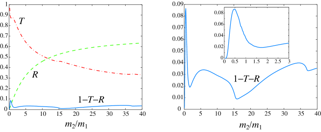
Figure 3: Left panel: the different fractions of the energy are plotted as a function of the mass ratio $\epsilon=m_{2}/m_{1}$. Right panel: trapped portion of the energy. The transmitted energy fraction $T$ of the right part of the chain is presented by the red dash-dotted line, the reflected part of the energy $R$ is given by the green dashed line, while the non-vanishing (for $\epsilon>0$) trapped fraction of the energy is shown by the blue solid line.

A well-understood limiting case is that of $\epsilon=0$, when $u_{0}=v_{0}$, so that the mass-with-mass defect is effectively absent and the system features near perfect transmission: $T\approx 1$ and $R\approx 0$. This observation takes into account the well-known feature hinch that over $99$% of the impact kinetic energy is stored within a highly nonlinear traveling wave (originally described by Nesterenko within his quasicontinuum theory nesterenko1 ). Another physical limit is that of large values of $\epsilon$, $m_{2}\gg m_{1}$, when the inertia prevents the secondary mass from moving, so $v_{0}\approx 0$. In this case the transmission is far from perfect (e.g. $T\approx 0.26$ and $R\approx 0.71$ at $\epsilon=10000$), and the trapped fraction of the energy approaches the value of about $0.03$ as $\epsilon$ becomes large. Observe that in the regime of comparable bead masses, between these two limits, the trapped energy fraction exhibits oscillations.

We begin by considering the case of small $\epsilon$. As $\epsilon$ departs from zero, we still have a single propagating traveling wave within the chain, but now it experiences a weak reflection from the defect. We also find that some of the energy is trapped, which is a fundamental difference from the observations in the context of light or heavy mass defects in a Hertzian chain hascoet ; job ; vakakis .

This picture is corroborated by the detailed dynamics of this case as presented in Fig. 4 for the value of $\epsilon=0.1$. The contour plot in the top left panel presents the space-time evolution of the velocity field which characteristically represents the traveling wave. The bottom left panel below the contour plot and on the same time scale shows the evolution of the quantities $(u_{n-1}-u_{n})_{+}$ and $(u_{n}-u_{n+1})_{+}$, which, as we recall, determine the forces exerted on the corresponding beads. When the force vanishes, there is what we call a “gap opening” theocharis_pre , i.e., the beads no longer interact. It is, thus, clear by also consulting the second and third subplots of Fig. 4 that upon the impact of the wave, there emerges a reflection and subsequently a permanent gap opening in the interaction of beads at $n=0$ and $n=-1$. This produces the single reflected pulse present in the process. On the other hand, there is a more prolonged interaction between beads at $n=0$ and $n=1$, which, in turn, leads at the early stage of the dynamics to the emergence of a transmitted pulse. However, a key feature also arising in the process is the existence of a trapped part of the energy. For the small $\epsilon$ considered here, this part is weak but it is definitely present and manifests itself as oscillations at a characteristic frequency. Interestingly, this frequency, as we will justify in Sec. IV where we analyze this asymptotic case, is precisely the linear frequency of the mass-with-mass oscillator $\omega=\sqrt{1+\epsilon^{-1}}$.

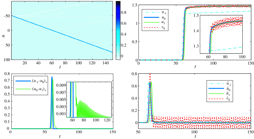
Figure 4: The results of simulations at $\epsilon=0.1$. The top left panel presents the space-time ($n$-$t$) evolution of the contour plot of the field $\dot{u}_{n}(t)$. The thick blue and green lines in the bottom left panel show the quantities $(u_{n-1}-u_{n})_{+}$ and $(u_{n}-u_{n+1})_{+}$, respectively, to give a sense of when (after the impact) gap openings arise. The top right panel presents the displacements of the central sites; cyan dash-dotted line corresponds to $u_{-1}(t)$, thick blue solid to $u_{0}(t)$, green solid to $u_{1}(t)$ and red dashed to $v_{0}(t)$. The same pattern is followed for the corresponding velocities at the bottom right plot.

We now turn to the opposite limit, namely that of a much larger mass $m_{2}$ in comparison to the mass $m_{1}$ of the granular chain beads. This case is represented by Fig. 5, which presents the computations for $\epsilon=10000$.

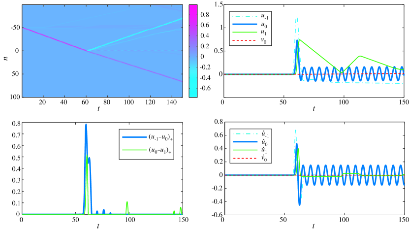
Figure 5: The same properties as for the Fig. 4 are illustrated but now for the case of $\epsilon=10000$.

In this case the large secondary mass barely moves ($v_{0}\approx 0$). However, $u_{0}$ oscillates around the zero value after the initial solitary wave reaches the defect site, triggering oscillations of $u_{1}$, whose amplitude descreases with time. As before, the gap between $n=0$ and $n=-1$ forms, sending a reflected pulse (note, however, the gap is no longer permanent, as these two sites briefly interact several times later). As in the small $\epsilon$ case, there is also a transmitted pulse in this limit. However, the transmitted pulse is much weaker in this case, while the reflected pulse is much stronger: indeed, at $\epsilon=10000$, we have $R\approx 0.71$ and $T\approx 0.26$, far from the near-perfect transmission we observed at small $\epsilon$. It is also important to note that there is an immediate gap opening, upon the first passage of the wave, between $n=0$ and $n=1$ in this case, as can be observed in Fig. 5. In this case, the asymptotic scenario (of $\epsilon\rightarrow\infty$) leads the central site to acquire a residual oscillation of $u_{0}$ with approximately unit frequency, while $v_{0}\rightarrow 0$. In that light, the system to consider analytically must include the beads $n=-1$, $n=0$ and $n=1$ for the $u$-field only. However, we were unable to identify an analytical solution of this six-dimensional nonlinear system (note also that unlike the reduced model considered in Sec. IV for small $\epsilon$, in this case there is no small parameter). Nevertheless, numerical computations with the single component system (where there exists a local oscillator at $n=0$) clearly confirm the validity of the above picture.

We now examine the interaction of the traveling wave with the defect for intermediate values of $\epsilon$. We start with the case $\epsilon=10$ shown in Fig. 6, when the secondary mass is still considerably larger than the primary one. First, it should be noted that as expected here, the fast-scale oscillations are performed by the mass $m_{1}$ (contrary to what was the case for small $\epsilon$, where the mass $m_{2}$ was the one performing the fast-scale vibrations). Second, the phenomena observed in this case are significantly different from what we have seen at small $\epsilon$. There still exists a small fraction of the energy which remains trapped at the central site. However, the principal phenomenology does not consist of a single transmitted and reflected wave, as was the case for small $\epsilon$. In this case, the dominant reflected wave may be a single one, as was the case for small $\epsilon$ (as shown in Fig. 6), but there is a cascade of transmitted waves which are somewhat reminiscent of the corresponding train of transmitted solitary waves discussed in hascoet for large mass defects in Hertzian chains; see also the work of sen for a similar problem where a solitary wave train also emerges as a consequence of a chain being stricken by a heavier bead, a role that in our system is played by the defect bead. The top right panel of the figure illustrates the displacements and allows the observation of the gap openings where there is no force after the impact of the traveling wave. We see that upon the transmission of the original traveling wave, there is a gap opening between the defect site and its left neighbor ($n=0$ and $n=-1$; see the thick blue curve in the bottom left panel in Fig. 6), which initiates the principal reflected wave traveling to the left. These two sites never interact again. However, the interaction of the $n=0$ defect site with the site to the right of it ($n=1$) is different. What is observed is that there is a series of gap openings which are followed (each in turn) by subsequent compression intervals (see the thin green curve in the bottom left panel). Each one of these sequences produces a new traveling wave, as can be seen in the top left panel. However, naturally, as the energy trapped within the central site keeps decreasing upon the release of subsequent traveling waves, the amplitude of each later (emerging) wave in the sequence is weaker than that of its predecessors and hence its speed is also smaller. This, in turn, justifies this sequence of decreasing amplitude and speed traveling waves emitted by the defect.

We note that a similar sequence of gap openings between the beads at $n=0$ and $n=1$ was also seen at $\epsilon=0.1$ (see the thin green curve in the inset in the bottom left panel Fig. 4). However, due to the much smaller amplitude and higher frequency of oscillations of $u_{0}(t)$ in that case, the nonzero interaction forces during the compression intervals and the duration of these intervals were too small to initiate additional traveling waves.

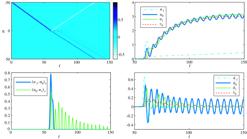
Figure 6: The same properties as for the Fig. 4 are illustrated but now for the case of $\epsilon=10$. Here, it is the lighter mass $m_{1}$ executing the fast scale oscillations, while opening a gap from the site to its left and presenting a cascade of alternating gap openings and compression events with its right neighbor which, in turn, lead to the successive emission of progressively smaller amplitude (and thus slower) waves within the solitary wave train that emerges in the space-time contour plot.

The dynamics for the case when the two masses are comparable is represented in Fig. 7, which corresponds to the value $\epsilon=0.5$. It should be noted here that this case represents the parameter close to the value at which the trapping fraction of the energy is maximal. In particular, as observed in Fig. 3, there is a clearly defined maximum in the fraction of energy that can be trapped by the system; this is another unique feature of our system. Not only can energy be trapped by the mass-with-mass defect but the trapping has a non-monotonic dependence on the ratio of the masses. As illustrated in the figure, here the scenario is different than the ones observed before. Here, the defect bead does not lead to a gap opening with respect to the bead to its left, but rather (predominantly) with respect to the bead to its right. In this case, we observe a two-peaked structure in $(u_{1}-u_{0})_{+}$ (see the bottom left panel of Fig. 7) which appears to nucleate two traveling waves moving in the right half of the chain. While a gap indeed opens past this principal interaction between $n=0$ and $n=1$, the beads do interact anew at a much later time (around $t=110$). Yet, similarly to the interactions shown in Fig. 4, such later (and considerably weaker) interactions do not produce appreciable solitary waves traveling to the right of $n=0$.

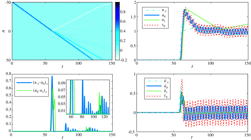
Figure 7: The case of $\epsilon=0.5$, close to the value at which the maximal trapping occurs. The same diagnostics as for $\epsilon=0.1$ in the case of Fig. 4 are shown. In this case the results reveal vibration over the fast scale of both $u_{0}$ and $v_{0}$ at the defect site and formation of only a second wave traveling to the right.

Finally, we turn to a setting where there exist additional defects within the chain. This is shown in Fig. 8, which contains both the case of two adjacent MwM defects (left panel), as well as that with three such adjacent defects (right panel). It can be clearly discerned that the addition of further defects significantly enhances the trapped fraction of the original energy within the defect sites. This fraction increases by about $10$% (for comparable values of $m_{2}/m_{1}$), when the defective region expands from one to two sites, and a comparable increase is observed when a third site is added. It is observed that this increase is at the expense of the transmitted fraction, which is well below $20$% ($\approx 15$% and well below the trapped fraction) for the three-MwM defect case. Interestingly, the trapped fraction preserves its oscillatory structure (notice that a less pronounced, yet somewhat similar variation is observed in the transmitted fraction), but the peak locations vary, as the number of defect sites is increased; e.g. the first, most pronounced peak occurs at larger values of $m_{2}/m_{1}$.

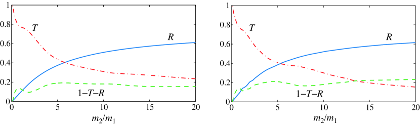
Figure 8: The same diagnostics as those of Fig. 3 are shown here (transmitted $T$, reflected $R$ and trapped $1-T-R$ fractions of the energy) as a function of the mass ratio, but now for the case of two adjacent mass defects (left) and that of three adjacent mass defects (right).

IV Analysis of the small mass ratio case

We now present a theoretical formulation which enables a semi-quantitative understanding of the situation at hand for the case of small $\epsilon$. We will use two different approaches, one of which involves perturbation analysis of the full system and the other is based on multiscale analysis of a reduced system.

IV.1 Perturbation analysis

Assume that there exists a traveling wave satisfying the standard Hertzian chain equation $\ddot{u}_{n}=(u_{n-1}-u_{n})^{3/2}_{+}-(u_{n}-u_{n+1})^{3/2}_{+}$, where the solution can be well approximated by the Nesterenko solitary wave nesterenko1 with

$$\dot{u}_{n}=\begin{cases}Ac\sin^{4}\biggl{(}\sqrt{\dfrac{2}{5}}(n-c(t-t_{0}))\biggr{)},&t_{0}+\dfrac{n-\sqrt{\frac{5}{2}}\pi}{c}\leq t\leq t_{0}+\dfrac{n}{c},\\ 0,&\text{otherwise}\end{cases}$$ (12)

where $c^{2}=(4/5)A^{1/2}$ and $t_{0}$ is the time when the wave leaves the $n=0$ site. Now, focusing on the difference $w_{0}=u_{0}-v_{0}$, we note that it satisfies the equation

$$\ddot{w}_{0}+\omega^{2}w_{0}=(u_{-1}-u_{0})^{3/2}_{+}-(u_{0}-u_{1})^{3/2}_{+},$$ (13)

where

$$\omega=\sqrt{1+\epsilon^{-1}}$$

is the natural frequency of the MwM defect. While Eq.( 13) is exact, observe that to a leading order its right hand side can be approximated by $\ddot{u}_{0}$. This means that the linear oscillator is driven by the propagating traveling wave, which we further approximate by the above Nesterenko expression (12) at $n=0$, with $\ddot{u}_{0}$ obtained by differentiating (12) once with respect to time. Notice that this drive is only active within the time interval $[t_{0}-(\pi\sqrt{5/2}/c),t_{0}]$, i.e. as the wave passes over $n=0$ site.

Within this approximation, Eq. (13) can be solved exactly to give

$$w_{0}=\int_{0}^{t}\frac{\sin(\omega(t-\tau))}{\omega}\ddot{u}_{0}(\tau)d\tau.$$ (14)

This simplified model has the advantage that it can be evaluated explicitly:

$$w_{0}=\begin{cases}0,&t<t_{0}-\frac{\pi\sqrt{5}}{\sqrt{2}c}\\ \frac{Ac^{2}}{D}\biggl{(}\sqrt{10}(5\omega^{2}-32c^{2})\sin(2\phi)+\sqrt{\frac{5}{2}}(8c^{2}-5\omega^{2})\sin(4\phi)+\frac{96c^{3}}{\omega}\sin(\omega(\frac{\pi\sqrt{5}}{\sqrt{2}c}+t-t_{0}))\biggr{)},&t_{0}-\frac{\pi\sqrt{5}}{\sqrt{2}c}\leq t\leq t_{0}\\ -\frac{192Ac^{5}}{D\omega}\sin(\omega\frac{\pi\sqrt{5}}{2\sqrt{2}c})\cos(\omega(t-t_{0}+\frac{\pi\sqrt{5}}{2\sqrt{2}c})),&t>t_{0},\end{cases}$$ (15)

where $\phi=\sqrt{2/5}(c(t-t_{0}))$ and $D=256c^{4}-200c^{2}\omega^{2}+25\omega^{4}$. Note that it corroborates the numerical observation that the trapped oscillation of the mass-with-mass defect is executed with the natural frequency $\omega$ of the relevant oscillator.

The results of this approximation for small values of $\epsilon$ are illustrated in the example of Fig. 9.

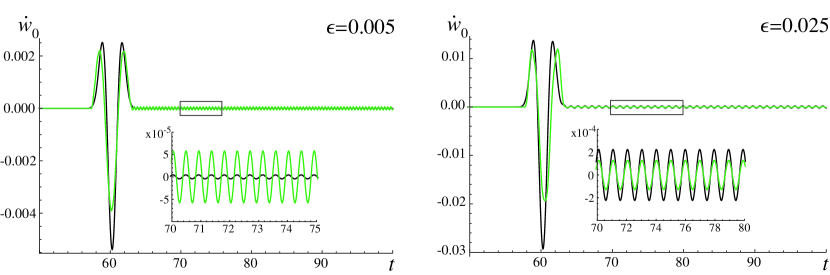
Figure 9: The time derivative of the difference $w_{0}(t)=u_{0}(t)-v_{0}(t)$ given by the direct numerical computation (black) and the analytical approximation (green) for $\epsilon=0.005$ and $\epsilon=0.025$. The insets zoom in on the regions inside the rectangles.

Here the traveling wave is initiated by the standard initial condition above and its resulting speed $c$ and amplitude $A$ are computed from the simulation prior to its impact with the mass-with-mass defect (we obtain $c\approx 0.841$ and $A\approx 0.811$). Then the time derivative of the expression of Eq. (15) (shown by the green line) is evaluated and compared, after an appropriate time shift $t_{0}$, with the direct result of the numerical simulation (black line) at the central site. It can be seen that the analytical solution captures the numerical result quite well qualitatively and, as expected, properly captures the frequency of the residual vibration trapped at the central site. It does not, however, capture its amplitude in general, which can be either larger (see, for example, the discrepancy at $\epsilon=0.005$) or smaller (e.g. $\epsilon=0.025$) than the numerical value. It also underestimates the amplitude of the large pulse that precedes it. This happens because our approximation neglects the effect the defect has on the propagating wave which adjusts its speed and shape prior to reaching the $n=0$ site.

IV.2 Small $\epsilon$ limit: two-bead problem

To better understand the small $\epsilon$ limit, we now turn to a simplification of the original problem in which we only consider the system involving two beads. Neglecting the left part of the chain can be justified by the fact that the numerical simulations show that after the defect bead has been kicked by the previous one, there is a gap opening between the two and therefore they do not interact again. Hence, the simplest configuration that could capture the transmission of the wave from $n=0$ to $n=1$, as well as the trapping of the energy in the $n=0$ site would be the two-site setting examined below. Importantly, these two phenomena exhibit a separation of time scales: the oscillation within the defect bead is one of a fast time scale, while the interaction between $n=0$ and $n=1$ occurs in a slower time scale, enabling the multiscale analysis presented below.

The simplified dynamical equations then read:

$$\begin{split}\ddot{u}_{0}&=-(u_{0}-u_{1})^{3/2}_{+}-(u_{0}-v_{0})\\ \epsilon\ddot{v}_{0}&=u_{0}-v_{0}\\ \ddot{u}_{1}&=(u_{0}-u_{1})^{3/2}_{+}.\end{split}$$ (16)

In considering this reduced model, we follow the approach in vakakis for a problem with a light mass defect, with the goal to qualitatively capture the dynamics of the system during an initial time period after the propagating wave reaches the mass-with-mass defect. For example, consider the initial conditions (emulating the kick provided through the gap-opening interaction with $n=-1$)

$$u_{0}(0)=v_{0}(0)=u_{1}(0)=\dot{v}_{0}(0)=\dot{u}_{1}(0)=0,\quad\dot{u}_{0}(0)=1.$$ (17)

The numerical solution of the system (16) at $\epsilon=0.01$ and $\epsilon=0.1$ subject to (17) is shown in Fig. 10.

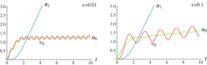
Figure 10: Numerical solution of (16), (17) at $\epsilon=0.01$ and $\epsilon=0.1$.

By numerically integrating the simplified system and comparing the results with the previously obtained ones for the full system, we see that the simplified model qualitatively captures the behavior of the full system at small $\epsilon$ in that $v_{0}(t)$ and $u_{0}(t)$ both oscillate, $v_{0}(t)$ with a larger amplitude, about some average value that increases with time, initially rapidly and then more slowly.

To analytically approximate (16) at small $\epsilon$, we use a two-timing approach vakakis . We introduce the fast time $\tau=t/\sqrt{\epsilon}$. This rescaling of time yields:

$$\begin{split}\dfrac{d^{2}u_{0}}{d\tau^{2}}&=-\epsilon(u_{0}-u_{1})^{3/2}_{+}-\epsilon(u_{0}-v_{0})\\ \dfrac{d^{2}v_{0}}{d\tau^{2}}&=u_{0}-v_{0}\\ \dfrac{d^{2}u_{1}}{d\tau^{2}}&=\epsilon(u_{0}-u_{1})^{3/2}_{+}.\end{split}$$ (18)

Substituting the expansion

$$\begin{split}u_{0}(\tau)&=U_{0}^{(0)}(\tau,t)+\sqrt{\epsilon}U_{0}^{(1)}(\tau,t)+\epsilon U_{0}^{(2)}(\tau,t)+\epsilon^{3/2}U_{0}^{(3)}(\tau,t)+O(\epsilon^{2})\\ v_{0}(\tau)&=V_{0}^{(0)}(\tau,t)+\sqrt{\epsilon}V_{0}^{(1)}(\tau,t)+\epsilon V_{0}^{(2)}(\tau,t)+\epsilon^{3/2}V_{0}^{(3)}(\tau,t)+O(\epsilon^{2})\\ u_{1}(\tau)&=U_{1}^{(0)}(\tau,t)+\sqrt{\epsilon}U_{1}^{(1)}(\tau,t)+\epsilon U_{1}^{(2)}(\tau,t)+\epsilon^{3/2}U_{1}^{(3)}(\tau,t)+O(\epsilon^{2})\end{split}$$

in (18), expanding the right hand side in terms of $\epsilon$ and keeping the terms up to $O(\epsilon^{2}$), we obtain

$$\begin{split}\dfrac{\partial^{2}U_{0}^{(0)}}{\partial\tau^{2}}&+\sqrt{\epsilon}\left(\dfrac{\partial^{2}U_{0}^{(1)}}{\partial\tau^{2}}+2\dfrac{\partial^{2}U_{0}^{(0)}}{\partial\tau\partial t}\right)+\epsilon\left(\dfrac{\partial^{2}U_{0}^{(0)}}{\partial t^{2}}+2\dfrac{\partial^{2}U_{0}^{(1)}}{\partial t\partial\tau}+\dfrac{\partial^{2}U_{0}^{(2)}}{\partial\tau^{2}}\right)+\epsilon^{3/2}\left(\dfrac{\partial^{2}U_{0}^{(1)}}{\partial t^{2}}+2\dfrac{\partial^{2}U_{0}^{(2)}}{\partial t\partial\tau}+\dfrac{\partial^{2}U_{0}^{(3)}}{\partial\tau^{2}}\right)\\ &=-\epsilon\left\{\left(U_{0}^{(0)}-U_{1}^{(0)}\right)_{+}^{3/2}+U_{0}^{(0)}-V_{0}^{(0)}\right\}-\epsilon^{3/2}\left\{\dfrac{3}{2}\left(U_{0}^{(0)}-U_{1}^{(0)}\right)_{+}^{1/2}\left(U_{0}^{(1)}-U_{1}^{(1)}\right)+U_{0}^{(1)}-V_{0}^{(1)}\right\}\end{split}$$

$$\begin{split}\dfrac{\partial^{2}V_{0}^{(0)}}{\partial\tau^{2}}&+\sqrt{\epsilon}\left(\dfrac{\partial^{2}V_{0}^{(1)}}{\partial\tau^{2}}+2\dfrac{\partial^{2}V_{0}^{(0)}}{\partial\tau\partial t}\right)+\epsilon\left(\dfrac{\partial^{2}V_{0}^{(0)}}{\partial t^{2}}+2\dfrac{\partial^{2}V_{0}^{(1)}}{\partial t\partial\tau}+\dfrac{\partial^{2}V_{0}^{(2)}}{\partial\tau^{2}}\right)+\epsilon^{3/2}\left(\dfrac{\partial^{2}V_{0}^{(1)}}{\partial t^{2}}+2\dfrac{\partial^{2}V_{0}^{(2)}}{\partial t\partial\tau}+\dfrac{\partial^{2}V_{0}^{(3)}}{\partial\tau^{2}}\right)\\ &=U_{0}^{(0)}-V_{0}^{(0)}+\sqrt{\epsilon}\left(U_{0}^{(1)}-V_{0}^{(1)}\right)+\epsilon\left(U_{0}^{(2)}-V_{0}^{(2)}\right)+\epsilon^{3/2}\left(U_{0}^{(3)}-V_{0}^{(3)}\right)\end{split}$$

$$\begin{split}\dfrac{\partial^{2}U_{1}^{(0)}}{\partial\tau^{2}}&+\sqrt{\epsilon}\left(\dfrac{\partial^{2}U_{1}^{(1)}}{\partial\tau^{2}}+2\dfrac{\partial^{2}U_{1}^{(0)}}{\partial\tau\partial t}\right)+\epsilon\left(\dfrac{\partial^{2}U_{1}^{(0)}}{\partial t^{2}}+2\dfrac{\partial^{2}U_{1}^{(1)}}{\partial t\partial\tau}+\dfrac{\partial^{2}U_{1}^{(2)}}{\partial\tau^{2}}\right)+\epsilon^{3/2}\left(\dfrac{\partial^{2}U_{1}^{(1)}}{\partial t^{2}}+2\dfrac{\partial^{2}U_{1}^{(2)}}{\partial t\partial\tau}+\dfrac{\partial^{2}U_{1}^{(3)}}{\partial\tau^{2}}\right)\\ &=\epsilon\left(U_{0}^{(0)}-U_{1}^{(0)}\right)_{+}^{3/2}+\dfrac{3}{2}\epsilon^{3/2}\left(U_{0}^{(0)}-U_{1}^{(0)}\right)_{+}^{1/2}\left(U_{0}^{(1)}-U_{1}^{(1)}\right)\end{split}$$

Then $O(1)$ problem reads

$$\dfrac{\partial^{2}U_{0}^{(0)}}{\partial\tau^{2}}=0,\quad\dfrac{\partial^{2}U_{1}^{(0)}}{\partial\tau^{2}}=0,\quad\dfrac{\partial^{2}V_{0}^{(0)}}{\partial\tau^{2}}=U_{0}^{(0)}-V_{0}^{(0)}$$ (19)

Solving the above equations and eliminating the secular terms (which feature unbounded growth in $\tau$), we obtain

$$U_{0}^{(0)}=B_{0}(t),\quad U_{1}^{(0)}=B_{1}(t)$$ (20)

and a fast oscillation of the defect as

$$V_{0}^{(0)}=C(t)\cos\tau+D(t)\sin\tau+B_{0}(t).$$ (21)

Next we consider the $O(\sqrt{\epsilon})$ problem:

$$\dfrac{\partial^{2}U_{0}^{(1)}}{\partial\tau^{2}}+2\dfrac{\partial^{2}U_{0}^{(0)}}{\partial\tau\partial t}=0,\quad\dfrac{\partial^{2}U_{1}^{(1)}}{\partial\tau^{2}}+2\dfrac{\partial^{2}U_{1}^{(0)}}{\partial\tau\partial t}=0,\quad\dfrac{\partial^{2}V_{0}^{(1)}}{\partial\tau^{2}}+2\dfrac{\partial^{2}V_{0}^{(0)}}{\partial\tau\partial t}=U_{0}^{(1)}-V_{0}^{(1)}$$ (22)

From (20), it follows that

$$\dfrac{\partial^{2}U_{0}^{(0)}}{\partial\tau\partial t}=\dfrac{\partial^{2}U_{1}^{(0)}}{\partial\tau\partial t}=0,$$

and hence the first two equations in (22) imply that

$$U_{0}^{(1)}=E_{0}(t),\quad U_{1}^{(1)}=E_{1}(t).$$ (23)

Differentiating (21) to find the mixed derivative in the third equation in (22),

$$\dfrac{\partial^{2}V_{0}^{(0)}}{\partial\tau\partial t}=-C^{\prime}(t)\sin\tau+D^{\prime}(t)\cos\tau,$$

we find that we must have $C^{\prime}(t)=D^{\prime}(t)=0$ in order to avoid secular terms in $V_{0}^{(1)}$. Thus $C$ and $D$ are constant, and we have

$$V_{0}^{(0)}=C\cos\tau+D\sin\tau+B_{0}(t),$$ (24)

while the last equation in (22) and (23) yield

$$V_{0}^{(1)}=F(t)\cos\tau+G(t)\sin\tau+E_{0}(t).$$ (25)

In the subsequent order, namely $O(\epsilon)$, we have

$$\begin{split}&\dfrac{\partial^{2}U_{0}^{(0)}}{\partial t^{2}}+2\dfrac{\partial^{2}U_{0}^{(1)}}{\partial t\partial\tau}+\dfrac{\partial^{2}U_{0}^{(2)}}{\partial\tau^{2}}=-\left(U_{0}^{(0)}-U_{1}^{(0)}\right)_{+}^{3/2}-\left(U_{0}^{(0)}-V_{0}^{(0)}\right)\\ &\dfrac{\partial^{2}V_{0}^{(0)}}{\partial t^{2}}+2\dfrac{\partial^{2}V_{0}^{(1)}}{\partial t\partial\tau}+\dfrac{\partial^{2}V_{0}^{(2)}}{\partial\tau^{2}}=U_{0}^{(2)}-V_{0}^{(2)}\\ &\dfrac{\partial^{2}U_{1}^{(0)}}{\partial t^{2}}+2\dfrac{\partial^{2}U_{1}^{(1)}}{\partial t\partial\tau}+\dfrac{\partial^{2}U_{1}^{(2)}}{\partial\tau^{2}}=\left(U_{0}^{(0)}-U_{1}^{(0)}\right)_{+}^{3/2}\end{split}$$ (26)

Using (20), (23) and recalling the third equation in (19), we can rewrite the first equation in (26) as

$$\dfrac{\partial^{2}}{\partial\tau^{2}}\left(U_{0}^{(2)}+V_{0}^{(0)}\right)=-B_{0}^{\prime\prime}(t)-(B_{0}(t)-B_{1}(t))_{+}^{3/2}.$$

To eliminate secular terms from $U_{0}^{(2)}$, we must then set the right hand side of this equation to zero:

$$B_{0}^{\prime\prime}(t)=-(B_{0}(t)-B_{1}(t))_{+}^{3/2}.$$ (27)

Elimination of the linear term in $\tau$ then means that $U_{0}^{(2)}+V_{0}^{(0)}$ is a function of $t$ only, yielding

$$U_{0}^{(2)}=H_{0}(t)-C\cos\tau-D\sin\tau,$$ (28)

where we used (24). Similarly, using (20) and (23) in the last equation of (26) and eliminating the secular terms in $U_{1}^{(2)}$, we obtain

$$B_{1}^{\prime\prime}(t)=(B_{0}(t)-B_{1}(t))_{+}^{3/2}$$ (29)

and

$$U_{1}^{(2)}=H_{1}(t).$$ (30)

Considering now the second equation in (26) and substituting the mixed derivative of (25) and (28), we have

$$\dfrac{\partial^{2}V_{0}^{(2)}}{\partial\tau^{2}}+V_{0}^{(2)}=-(2G^{\prime}(t)+C)\cos\tau+(2F^{\prime}(t)-D)\sin\tau+H_{0}(t)-B_{0}^{\prime\prime}(t).$$

To avoid secular terms, we must set the coefficients in front of $\sin\tau$ and $\cos\tau$ in the right hand side to zero, which yields $F(t)=(D/2)t+D_{0}$ and $G(t)=-(C/2)t+C_{0}$, where $C_{0}$ and $D_{0}$ are constant. Thus we have

$$V_{0}^{(1)}=\left(\dfrac{D}{2}t+D_{0}\right)\cos\tau+\left(C_{0}-\dfrac{C}{2}t\right)\sin\tau+E_{0}(t),$$ (31)

while

$$V_{0}^{(2)}=I(t)\cos\tau+J(t)\sin\tau+H_{0}(t)-B_{0}^{\prime\prime}(t).$$

Finally, we turn to the $O\left(\epsilon^{3/2}\right)$ problem:

$$\begin{split}&\dfrac{\partial^{2}U_{0}^{(1)}}{\partial t^{2}}+2\dfrac{\partial^{2}U_{0}^{(2)}}{\partial t\partial\tau}+\dfrac{\partial^{2}U_{0}^{(3)}}{\partial\tau^{2}}=-\dfrac{3}{2}\left(U_{0}^{(0)}-U_{1}^{(0)}\right)_{+}^{1/2}\left(U_{0}^{(1)}-U_{1}^{(1)}\right)-\left(U_{0}^{(1)}-V_{0}^{(1)}\right)\\ &\dfrac{\partial^{2}V_{0}^{(1)}}{\partial t^{2}}+2\dfrac{\partial^{2}V_{0}^{(2)}}{\partial t\partial\tau}+\dfrac{\partial^{2}V_{0}^{(3)}}{\partial\tau^{2}}=U_{0}^{(3)}-V_{0}^{(3)}\\ &\dfrac{\partial^{2}U_{1}^{(1)}}{\partial t^{2}}+2\dfrac{\partial^{2}U_{1}^{(2)}}{\partial t\partial\tau}+\dfrac{\partial^{2}U_{1}^{(3)}}{\partial\tau^{2}}=\dfrac{3}{2}\left(U_{0}^{(0)}-U_{1}^{(0)}\right)_{+}^{1/2}\left(U_{0}^{(1)}-U_{1}^{(1)}\right)\end{split}$$ (32)

Proceeding as in the $O(\epsilon)$ case, we use (23), (28), the third equation in (22) and (24) to rewrite the first equation in (32) as

$$\dfrac{\partial^{2}}{\partial\tau^{2}}\left(U_{0}^{(3)}+V_{0}^{(1)}\right)=-E_{0}^{\prime\prime}(t)-\dfrac{3}{2}\left(B_{0}(t)-B_{1}(t)\right)_{+}^{1/2}(E_{0}(t)-E_{1}(t)).$$

To eliminate secular terms from $U_{0}^{(3)}$, we must then set the right hand side of this equation to zero:

$$E_{0}^{\prime\prime}(t)=-\dfrac{3}{2}\left(B_{0}(t)-B_{1}(t)\right)_{+}^{1/2}(E_{0}(t)-E_{1}(t)).$$ (33)

Then, again eliminating the secular terms, we get that $U_{0}^{(3)}+V_{0}^{(1)}$ is only a function of $t$, which in light of (31) yields

$$U_{0}^{(3)}=K_{0}(t)-\left(\dfrac{D}{2}t+D_{0}\right)\cos\tau-\left(C_{0}-\dfrac{C}{2}t\right)\sin\tau.$$

Similarly, (23), (30) and the last equation in (32) result in

$$E_{1}^{\prime\prime}(t)=\dfrac{3}{2}\left(B_{0}(t)-B_{1}(t)\right)_{+}^{1/2}(E_{0}(t)-E_{1}(t))$$ (34)

and $U_{1}^{(3)}=K_{1}(t)$.

So up to order $O(\epsilon)$ we have

$$\begin{split}u_{0}(t)&=B_{0}(t)+\sqrt{\epsilon}E_{0}(t),\quad u_{1}(t)=B_{1}(t)+\sqrt{\epsilon}E_{1}(t),\\ v_{0}(t)&=B_{0}(t)+C\cos\dfrac{t}{\sqrt{\epsilon}}+D\sin\dfrac{t}{\sqrt{\epsilon}}+\sqrt{\epsilon}\left\{E_{0}(t)+\left(D_{0}+\dfrac{D}{2}t\right)\cos\dfrac{t}{\sqrt{\epsilon}}+\left(C_{0}-\dfrac{C}{2}t\right)\sin\dfrac{t}{\sqrt{\epsilon}}\right\},\end{split}$$

where $B_{0}(t)$, $B_{1}(t)$ are found by solving (27), (29), $E_{0}(t)$, $E_{1}(t)$ satisfy (33), (34), and the initial conditions for these functions, as well as the constants $D_{0}$, $D$, $C_{0}$, $C$, are found from the initial conditions for $u_{0}(t)$, $u_{1}(t)$ and $v_{0}(t)$.

Now we consider the initial conditions (17). Then $u_{0}(0)=v_{0}(0)=u_{1}(0)=0$, which imply that $B_{0}(0)=B_{1}(0)=E_{0}(0)=E_{1}(0)=0$ and $C=D_{0}=0$. The initial condition $\dot{u}_{0}(0)=1$ implies $B_{0}^{\prime}(0)=1$ and $E_{0}^{\prime}(0)=0$, while $\dot{u}_{1}(0)=0$ implies $B_{1}^{\prime}(0)=E_{1}^{\prime}(0)=0$. Differentiating $v_{0}(t)$ and using $\dot{v}_{0}(0)=0$ and the above results, we get

$$\dot{v}_{0}(0)=1+\dfrac{D}{\sqrt{\epsilon}}+C_{0}+\dfrac{D\sqrt{\epsilon}}{2}=0,$$

which implies $D=0$ and $C_{0}=-1$. Since $E_{0}(t)$, $E_{1}(t)$ satisfy the linear system (33), (34) subject to the zero initial conditions, they must vanish. Thus we have

$$u_{0}(t)=B_{0}(t),\quad u_{1}(t)=B_{1}(t),\quad v_{0}(t)=B_{0}(t)-\sqrt{\epsilon}\sin\dfrac{t}{\sqrt{\epsilon}}$$ (35)

where $B_{0}(t)$, $B_{1}(t)$ satisfy (27), (29) and the initial conditions $B_{0}(0)=B_{1}(0)=B_{1}^{\prime}(0)=0$ and $B_{0}^{\prime}(0)=1$. To solve this problem, it is convenient to introduce the new variables $y_{0}(t)=(B_{0}(t)-B_{1}(t))/2$ and $z_{0}(t)=(B_{0}(t)+B_{1}(t))/2$. Then $z_{0}(t)$ satisfies $z_{0}^{\prime\prime}(t)=0$, $z_{0}(0)=0$, $z_{0}^{\prime}(0)=1/2$, so we have $z(t)=t/2$. Meanwhile, $y_{0}(t)$ solves

$$y_{0}^{\prime\prime}+(2y_{0})_{+}^{3/2}=0,\quad y_{0}(0)=0,\quad y_{0}^{\prime}(0)=1/2.$$ (36)

When $y_{0}>0$, it satisfies $y_{0}^{\prime\prime}+(2y_{0})^{3/2}=0$, which together with the initial conditions implies that it lies on the trajectory

$$(y_{0}^{\prime})^{2}+\dfrac{8}{5}\sqrt{2}y_{0}^{5/2}=\dfrac{1}{4}$$

This can be solved for $t$ as a function of $y_{0}$ in terms of hypergeometric functions. We obtain

$$t=\begin{cases}2y_{0}\,{}_{2}F_{1}[\frac{2}{5},\frac{1}{2},\frac{7}{5},\frac{32}{5}\sqrt{2}y_{0}^{5/2}],&0\leq t\leq t_{*}\\ 2(t_{*}-y_{0}\,{}_{2}F_{1}[\frac{2}{5},\frac{1}{2},\frac{7}{5},\frac{32}{5}\sqrt{2}y_{0}^{5/2}]),&t_{*}\leq t\leq 2t_{*},\end{cases}$$ (37)

where $t_{*}=2y_{0}\,{}_{2}F_{1}[\frac{2}{5},\frac{1}{2},\frac{7}{5},1]$ is such that $y_{0}(t_{*})=y_{0}^{*}=\left(\dfrac{5}{32\sqrt{2}}\right)^{2/5}$ For $t>2t_{*}$ we have $y_{0}^{\prime\prime}=0$, and since $y_{0}^{\prime}(2t_{*})=-1/2$ and $y_{0}(2t_{*})=0$, this yields

$$y_{0}(t)=t_{*}-t/2\quad\text{for $t>2t_{*}$}.$$ (38)

Recalling that $B_{0}(t)=y_{0}(t)+z_{0}(t)$ and $B_{1}(t)=z_{0}(t)-y_{0}(t)$, we obtain

$$u_{0}(t)=\dfrac{t}{2}+y_{0}(t),\quad u_{1}(t)=\dfrac{t}{2}-y_{0}(t),\quad v_{0}(t)=\dfrac{t}{2}+y_{0}(t)-\sqrt{\epsilon}\sin\dfrac{t}{\sqrt{\epsilon}}$$ (39)

where $y_{0}(t)$ is given by (37), (38). In particular, for $t\geq 2t_{*}$ we have $u_{0}$ becomes constant, $u_{0}(t)=t_{*}$, while $u_{1}$ linearly increases, $u_{1}(t)=t_{*}+t/2$.

The comparison of the approximation (39) (black curves) and the numerical solution (colored curves) is shown in Fig. 11 at $\epsilon=0.01$.

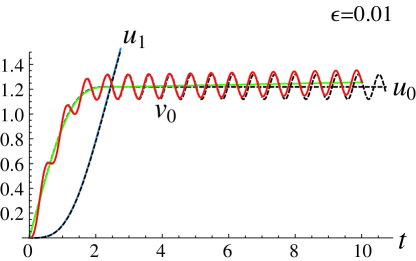
Figure 11: Comparison of the numerical solution of (16), (17) at $\epsilon=0.01$ (colored solid curves) and the two-timing approximation up to $O(\epsilon)$ (black dashed curves).

One can see that the approximation works very well for $t<5$, but starts deviating for larger $t$ because it does not capture the slight increase in $u_{0}(t)$ for $t>2t_{*}$. It also does not capture the small-amplitude oscillations of $u_{0}(t)$, which become visible at larger $\epsilon$; see, for example, Fig. 10 at $\epsilon=0.1$. To capture these effects, one needs to include higher-order terms. Note, however, that the function $(u_{0}-u_{1})^{3/2}_{+}$ is not smooth at zero and cannot be expanded beyond the first derivative term at this point. Hence, while this approach is valuable in analytical understanding of the leading order dynamics in the simplified two-site system, it also has its limitations with respect to some of the higher order effects therein.

Nevertheless, the analytical approximations considered in this section offer a detailed quantitative picture of the energy trapping and residual oscillatory dynamics within the defect (and capture its frequency), as well as of the detailed exchange dynamics between sites $n=0$ and $n=1$.

V Conclusions and Future Challenges

In the present work, we have explored the propagation of waves in a granular chain in which a mass-with-mass defect is present. In this setting, a local oscillator with additional parameters arises, the most significant of which is the ratio between the mass-with-mass defect and that of the rest of the masses within the chain. We have considered the problem as a function of this parameter numerically and wherever possible also analytically.

We found that in the case of the small defect to bead mass ratio, the traveling wave remains essentially unaltered, except for the fact that a part of its energy is reflected and a part of its energy is trapped in the form of localized oscillation. The trapping of energy is an exclusive feature of this system that was not observed in chains containing mass defects. This phenomenon was studied analytically in two distinct ways. One of them involved a direct perturbative approach based on the fact that the local oscillator is principally driven by the weakly affected (in this case) solitary wave. The second one was a multiscale technique applied on a reduced, two-beads system based on two-timing which revealed the key role of the dynamics/interaction of the defect site $n=0$ with the following one ($n=1$). We also studied the effect of the defect for all the representative values of the mass ratio using numerical methods. In the limit of very large mass ratio, we found that the reflection is more significant than the transmission and a considerable amount of trapping still occurs. In the intermediate mass ratio cases we found the potential of exciting multiple waves either one directly after the other, or through a sequence of gap openings leading to a train of solitary waves emitted towards the right of the defect. In each case, we studied the dynamics of the interaction with the defect by computing the trajectories of the beads in the vicinity of the defect ($n=-1$, $n=0$ and $n=1$).

The present study suggests many possible future investigations on systems containing MwM defects. On one hand, the large mass ratio limit would certainly be worthwhile to consider analytically. We also found that the energy trapped in the MwM defect shows a non-monotonic dependence on the mass ratio which has not yet been explained. And finally, this study could be extended to cover the propagation of traveling waves in ordered systems where all the beads have a MwM defect. These topics are currently under consideration and will be reported in future publications.

Acknowledgements. CD acknowledges support from the National Science Foundation, grant number CMMI-844540 (CAREER) and NSF 1138702. PGK acknowledges support from the US National Science Foundation under grant CMMI-1000337, the US Air Force under grant FA9550-12-1-0332, the Alexander von Humboldt Foundation, as well as the Alexander S. Onassis Public Benefit Foundation. The work of AV was supported by the NSF grant DMS-1007908.

References

- (1) V. F. Nesterenko, Dynamics of Heterogeneous Materials (Springer-Verlag, New York, NY, 2001).
- (2) S. Sen, J. Hong, J. Bang, E. Avalos, and R. Doney, Phys. Rep. 462, 21 (2008).
- (3) C. Daraio, V. F. Nesterenko, E. B. Herbold, and S. Jin, Phys. Rev. E. 73, 026610 (2006).
- (4) C. Coste, E. Falcon, and S. Fauve, Phys. Rev. E. 56, 6104 (1997)
- (5) C. Daraio, V. F. Nesterenko, E. B. Herbold, and S. Jin, Phys. Rev. Lett. 96, 058002 (2006).
- (6) J. Hong, Phys. Rev. Lett. 94, 108001 (2005).
- (7) F. Fraternali, M. A. Porter, and C. Daraio, Mech. Adv. Mat. Struct. 17(1), 1 (2010).
- (8) R. Doney and S. Sen, Phys. Rev. Lett. 97, 155502 (2006).
- (9) D. Khatri, C. Daraio, and P. Rizzo, SPIE 6934, 69340U (2008).
- (10) C. Daraio, V. F. Nesterenko, E. B. Herbold, and S. Jin, Phys. Rev. E 72, 016603 (2005).
- (11) A. Spadoni, C. Daraio, Proc. of the Nat. Acad. of Sci., 107, 7230 (2010).
- (12) V. F. Nesterenko, C. Daraio, E. B. Herbold, and S. Jin, Phys. Rev. Lett. 95, 158702 (2005).
- (13) K. Ahnert and A. Pikovsky, Phys. Rev. E 79, 026209 (2009).
- (14) A. Rosas and K. Lindenberg, Phys. Rev. E 69, 037601 (2004).
- (15) E. Hascoët and H. J. Herrman, Eur. Phys. J. B 14, 183 (2000).
- (16) S. Job, F. Santibanez, F. Tapia and F. Melo, Phys. Rev. E 80, 025602 (2009)
- (17) Y. Starosvetsky, K. R. Jayaprakash, and A.F. Vakakis, J. Appl. Mech. 79, 01101 (2012).
- (18) G. Theocharis, M. Kavousanakis, P. G. Kevrekidis, C. Daraio, M.A. Porter, and I. G. Kevrekidis Phys. Rev. E 80, 066601 (2009).
- (19) N. Boechler, G. Theocharis, Y. Man, P.G. Kevrekidis and C. Daraio, arXiv:1103.2483.
- (20) N. Boechler, G. Theocharis, C. Daraio, Nature Materials 10, 665 (2011).
- (21) G. Theocharis, N. Boechler, P. G. Kevrekidis, S. Job, M.A. Porter, and C. Daraio Phys. Rev. E 82, 056604 (2010).
- (22) A. Sokolow, E. G. Bittle and S. Sen, EPL 77, 24002 (2007).
- (23) J. M. English and R. L. Pego, Proceedings of the AMS 133, 1763 (2005).
- (24) A. Stefanov and P. G. Kevrekidis, arXiv:1105.3364 (J. Nonlin. Sci., in press).
- (25) E. J. Hinch and S. Saint-Jean, Proc. R. Soc. Lond. A 455, 3201 (1999).
- (26) S. Sen, T. R. K. Mohan, P. Donald, S. Swaminathan, A. Sokolow, E. Avalos and M. Nakagawa. Int. J. Modern Phys. B, 19, 2951 (2005).
- (27) G. James, P.G. Kevrekidis, J. Cuevas, arXiv:1111.1857.