Balanced K-SAT and Biased random K-SAT on trees

Abstract

We study and solve some variations of the random $K$-satisfiability problem - balanced $K$-SAT and biased random $K$-SAT - on a regular tree, using techniques we have developed earlier ss . In both these problems, as well as variations of these that we have looked at, we find that the SAT-UNSAT transition obtained on the Bethe lattice matches the exact threshold for the same model on a random graph for $K=2$ and is very close to the numerical value obtained for $K=3$. For higher $K$ it deviates from the numerical estimates of the solvability threshold on random graphs, but is very close to the dynamical $1$-RSB threshold as obtained from the first non-trivial fixed point of the survey propagation algorithm.

Random $K$-Satisfiability is a random constraint satisfaction problem in which one tries to find a satisfying assignment for a randomly generated logical expression in conjugate normal form(CNF), which is an AND of $M$ clauses. Each clause consists of an OR of $K$ Boolean literals which are chosen randomly from a set of $N$ Boolean variables. As the constraint density ($\alpha=M/N$) increases, the number of satisfying assignments decreases. In the limit of $M\rightarrow\infty$ and $N\rightarrow\infty$, the system is known to have a sharp threshold in constraint density $\alpha_{c}$ below which the probability of finding satisfiable assignments approaches $1$ and above which it vanishes. msl ; kirkpatrick .

The problem is originally defined on a random graph, but because of the presence of loops, this is hard to solve exactly for arbitrary $K$. The location of a sharp threshold $\alpha_{c}$ is known rigorously for $K=2$ chvataletal . For higher $K$ only bounds on upper and lower thresholds are provenachlioptas_bounds . However using non-rigorous but powerful methods from statistical physics, namely the replica and cavity methods, estimates for the threshold are obtained which seem to be very close to the values obtained numerically mezard-science ; mmz ; monasson .

The replica and cavity methods also predict that the solvability threshold is only one of many thresholds that exist in the problem as the number of constraints is increased. Before the solvability transition occurs, it is conjectured that the set of solutions (or satisfying assignments) first breaks up into a large number of well separated clusters at the clustering transition $\alpha_{d}$ mezard-science ; biroli . As the number of constraints further increases, it is argued that there is first a condensation transition lenkaetal_pnas in which the number of clusters changes from from being exponentially numerous to sub-exponential and a freezing transition beyond which some variables take the same value in all the solutions of a given cluster semer ; lk . Though again, it is hard to prove rigorous results about the existence of these transitions on a random graph (however, in a recent result,coja-oghlan proves rigorously the existence of a clustering transition in some random constraint satisfaction problems) the cavity method is able to predict numbers very close to those observed numerically. In addition, it is conjectured mezard-montanari that the threshold for clustering on a random graph is exactly equal to the reconstruction threshold on the corresponding tree (roughly defined, a tree graph is said to be reconstructable if the value that the root takes can be determined by the variable values at the leaves), supplying a further motivation for comparing results obtained thoretically on tree graphs with those obtained numerically for random graphs.

Recently we have studied the random $K$-SAT defined on a regular $d$-ary rooted tree ss . By fixing the boundary we could calculate the moments of the number of solutions (averaged over all possible instances of the logical expression) exactly. Of more relevance to this paper, we also studied the probability (or fraction of instances) of having a satisfiable assignment as a function of tree depth. As expected, for a tree, this probability may be written as a recursion relating the distribution at one level of the tree to the next level. We solved for the fixed point of these recursions to find that the behaviour of the probability matches the behaviour of $K$-SAT on a random graph atleast qualitatively i.e, it shows a continuous transition for $K=2$ and a first order transition for $K\geq 3$. In addition we found that the value of $\alpha(K)$ at which this transition takes place is very close to the value of the dynamical transition $\alpha_{d}(K)$ obtained for random graphs using the cavity method.

In this paper we compute the same quantity (the fraction of satisfiable instances as a function of $d$) for some variants of the random $K$-SAT on a $d$-ary rooted tree and compare with the solvability thresholds obtained for the same problem on a regular random graph. We find that for $K=2$ the threshold obtained via the tree calculations matches the known exact value for a regular random graph. For higher $K$, we have studied the problem numerically on regular random graphs and find that the threshold estimated on the tree is very close to the threshold obtained numerically for $K=3$, though deviating more and more as $K$ increases. Interestingly, as before ss , the values obtained by our method are also very close to the value predicted for the clustering transition by dynamical $1$-RSB calculations on a random graph for these models (rm ; zdeborova ).

The two variants of $K$-SAT studied in this paper are Biased-random $K$-SAT and Balanced $K$-SAT. In biased random $K$-SAT each variable is negated with probability $p$ (for $p=1/2$ this reduces to the uniform random $K$-SAT). In Balanced $K$-SAT, each variable is constrained to occur negated and non-negated an equal number of times. We have also studied a generalisation of balanced $K$-SAT which we call $f$-balanced $K$-SAT, where a literal occurs $f$ times as one kind and $1-f$ as another.

The plan of the paper is as follows: In Section I we explain the $d$-ary rooted tree on which we define various variants of random $K$-SAT. In Section II and III we study the biased random $K$-SAT and balanced $K$-SAT on the tree and compare the SAT-UNSAT threshold on the tree with the thresholds obtained on random graphs and regular random graphs. In Section IV we explain the connection between our approach and the survey-propagation algorithm, which goes towards understanding why the numbers we get as an estimate of the solvability transition, also happen to be very close to the numbers obtained via dynamical 1-RSB calculations for the clustering transition.

I The model

Figure 1: $3$-SAT on a rooted tree of depth $2$ and $d=2$. Only the clauses neighboring the root are labelled. Surface variables (or leaves) are depicted by a $\bullet$. Variable $x_{0}$ is at depth $2$, variables $x_{1}-x_{4}$ are at depth $1$ and the leaves are at depth $0$. Dashed/full lines between a variable and a clause indicate that it is negated/non-negated.

We define the $K$-SAT problem on a tree as follows. Consider a regular $d$-ary tree $T$ in which every vertex has exactly $d$ descendents. The root of the tree $x_{0}$ has degree $d$ and its $d$ edges are connected to function nodes $\{c_{1},c_{2}...,c_{d}\}$. Each function node has degree $K$, and each of its $K-1$ descendents $\{x_{i}=x_{1},x_{2},....x_{k-1}\}$ is the root of an independent tree (see Fig. 1 ). Hence the root has a degree $d$ while all the other vertices on the tree (except the leaves which have a degree $=1$) have a degree $d+1$. Each vertex can take only two values: $-1$ or $1$. Each function node is associated independently with a clause $\phi(x_{0},x_{1},...,x_{k-1})=\ell_{0}\bigvee\ell_{1}\bigvee....\ell_{k-1}$. Here $\ell_{i}$ is one of the two literals $x_{i}$ or $\overline{x_{i}}$, depending on whether $x_{i}$ is joined to the function node by a dashed or a solid line (see Fig.  1).

An assignment $\sigma$ of all the variables on the tree is a solution iff $\phi=1$ for all the clauses on the tree. One configuration of dashed and solid lines on the tree defines a realization $R$.

We study the probability that a realization has no solution on this tree for a fixed boundary. A realization with no solution is one for which not a single assignment of the variables provides a solution. This can happen if there is even a single variable on the graph, which, whether it takes the value $-1$ or $1$, causes atleast one clause to be unsatisfied. Such a variable then is a variable that can take $0$ values by our definition, and a realization that is not solvable has at least one variable of this type.

On the tree graph, we can define the probabilities of a variable taking $0$, $1$ or $2$ values on the corresponding subtree. We define $p_{i}(0)$ as the conditional probability for a variable $x_{i}$ to cause a contradiction, in the subtree of which it is the root, given that all the other variables in the subtree can take at least $1$ value. We can then estimate the probability of a realization having a solution (or the fraction of realizations that have solutions) by calculating the quantity $\Pi_{x_{i}}(1-p_{i}(0))$ where the product is over all the variables in the graph. The tree structure of the graph, gives us a way of calculating $p_{i}(0)$ through recursions.

We define below some of the quantities in terms of which these recursions are written. We define $P_{n}(0)$ to be the probability that (or the fraction of realizations in which) a variable at depth $n$ can neither take the value $-1$ nor take the value $1$, without causing a contradiction in its subtree. Here, by depth $n$, we mean a node that is $n$ levels away from the leaves (see Fig.  1). Note that because of the tree structure and because of the definition of the specific quantity we are looking at, all variables $x_{i}$ at depth $n$ will have the same probability $P_{n}$. The probability that a variable at depth $n$, can take only one of the two values $-1$ or $1$ is defined to be $P_{n}(1)$ (the boundary nodes have $P_{0}(1)=1$, for example). Similarly the probability that a variable at depth $n$ can take both values is $P_{n}(2)=1-P_{n}(0)-P_{n}(1)$. For the problems we look at, we are interested in the recursions for these quantities deep within the tree, as in ss , so that we can get rid of boundary effects.

II Biased random K-SAT

We consider a model where each variable has a fixed degree $d+1$, and a variable appears as negated with probability p. For $p=1/2$ this corresponds to the uniform random K- SAT ss . This model was also studied in rm for $K=3$ on random graphs using the replica and cavity methods.

II.1 Biased random $K$-SAT on a tree

Let us first calculate $P_{n+1}(0)$ for variable $x_{0}$ (assuming it is at depth $n+1$), given these quantities for its descendents. Assume variable $x_{0}$ has a degree $d$ (by definition) and assume it is not negated on $d_{1}$ of these clauses. Variable $x_{0}$ will not be able to take the value $-1$ in the case when at least one of the $d_{1}$ clauses is not satisfied by the $K-1$ variables at the other end. In this case there will be at least one unsatisfied clause if $x_{0}$ takes the value $-1$. Similarly, if at least one of the $d-d_{1}$ clauses which are satisfied by $x_{0}$, are also not satisfied by the $K-1$ variables at the other end, then $x_{0}$ cannot take the value $1$ either.

It is easy to see that averaging over all realizations at depth $n+1$ implies averaging over all values of $d_{1}$, as well as averaging over all realizations at depth $n$. It is important to note however tha realizations at depth $n+1$ are only built up from those realizations at depth $n$ that do have solutions. We define $Q_{n}$ as the conditional probability that a depth $n$ variable does not satisfy the clause above (to depth $n+1$), given that it has to be able to take at atleast one value (which satisfies the sub tree of which it is the root). The recursion for $P_{n+1}(0)$ is then:

$$P_{n+1}(0) = \sum_{d_{1}=1}^{d_{1}=d-1}\left(\begin{array}[]{c}d\\ d_{1}\end{array}\right)p^{d_{1}}(1-p)^{d-d_{1}}(1-(1-Q_{n}^{K-1})^{d_{1}})(1-(1-Q_{n}^{K-1})^{d-d_{1}})$$ (3)

$$= 1+(1-Q_{n}^{K-1})^{d}-(1-pQ_{n}^{k-1})^{d}-(1-(1-p)Q_{n}^{k-1})^{d}$$ (4)

Now we define $P_{n+1,-}(1)$ as the probability that a variable takes only one value and that value is $-1$ and $P_{n+1,+}(1)$ as the probability that the variable takes only one value and that value is $1$. Hence, the probability that a variable can take only one of the two possible values is $P_{n+1}(1)=P_{n+1,-}(1)+P_{n+1,+}(1)$. Recursions for these two quantities are as follows:

$$P_{n+1,-}(1) = \sum_{d_{1}=0}^{d_{1}=d}\left(\begin{array}[]{c}d\\ d_{1}\end{array}\right)p^{d_{1}}(1-p)^{d-d_{1}}(1-(1-Q_{n}^{K-1})^{d_{1}})((1-Q_{n}^{K-1})^{d-d_{1}})$$ (7)

$$= (1-(1-p)Q_{n}^{K-1})^{d}-(1-Q_{n}^{K-1})^{d}$$ (8)

$$P_{n+1,+}(1) = \sum_{d_{1}=0}^{d_{1}=d}\left(\begin{array}[]{c}d\\ d_{1}\end{array}\right)p^{d_{1}}(1-p)^{d-d_{1}}(1-(1-Q_{n}^{K-1})^{d-d_{1}})((1-Q_{n}^{K-1})^{d_{1}})$$ (11)

$$= (1-pQ_{n}^{K-1})^{d}-(1-Q_{n}^{K-1})^{d}$$ (12)

Hence,

$$Q_{n+1}=\frac{pP_{n+1,+}(1)+(1-p)P_{n+1,-}(1)}{1-P_{n+1}(0)}$$ (13)

This gives us the recursion

$$Q_{n+1}=\frac{p(1-pQ_{n}^{K-1})^{d}+(1-p)(1-(1-p)Q_{n}^{K-1})^{d}-(1-Q_{n}^{K-1})^{d}}{(1-pQ_{n}^{K-1})^{d}+(1-(1-p)Q_{n}^{K-1})^{d}-(1-Q_{n}^{K-1})^{d}}$$ (14)

These equations are a generalization of the recursions for $Q_{n+1}$ obtained in ss for $p=1/2$. From these equations the threshold at which the fraction of realizations goes to zero exponentially with the depth of the tree may be extracted. This is the solvability threshold for these models kirkpatrick . A fixed point analysis of Eq. 14 predicts a continuous transition for $K=2$ and a first order transition for $K>2$ for all $0<p<1$ (We see no change in behaviour for any non-zero value of $p$ though, as reported in rm ). The value of $d$ at which the system undergoes a continuous transition for $K=2$ can be extracted by expanding to order $Q^{2}$ in Eq. 14 at the fixed point. This gives, for $K=2$:

$$Q_{c}=\frac{2(1-2dp+2dp^{2})}{3(d-1)d(p^{2}-p)}$$ (15)

which implies $d_{c}=\frac{1}{2p(1-p)}$.

II.2 Comparison with results on random graph

The calculations above should be compared with the value of the solvability threshold on a regular random graph. On general grounds, the value of $\alpha_{c}$ corresponding to the fixed point value $d_{c}$ on the tree should be $(d_{c}+1)/K$ baxter ; gujrati . Hence for $2$-SAT, $d_{c}=\frac{1}{2p(1-p)}$ is equivalent to $\alpha_{C}=1/2+1/(4p(1-p))$.

A known earlier result cooper provides us an opportunity to compare the above value of $\alpha$ with the exact value of the solvability threshold for $2$-SAT. Let $r_{i}$ represent the degree of $i^{th}$ variable on a random graph, and $r_{i,-}$ and $r_{i,+}$ be the degree of the corresponding literals. Hence $r_{i}=r_{i,-}+r_{i,+}$. For $2$-SAT defined on a random graph with a given literal distribution $R=\{r_{1,-},r_{1,+},....\}$, the location of the threshold can be derived using the following theorem by Cooper et al cooper :

Theorem: Let $R$ be any degree sequence over $N$ variables, with $\Delta=N^{1/11}$, and let $F$ be a uniform random simple formula with a given degree sequence $R$, then for $0<\epsilon<1$ and $N\rightarrow\infty$, if $D=\sum_{i}r_{i,-}r_{i,+}<(1-\epsilon)M$ then P(F is satisfiable) $\rightarrow 1$ and if $D>(1+\epsilon)M$ then P(F is satisfiable) $\rightarrow 0$. Here $M$ is the number of clauses.

The theorem can be easily generalised to the case where we take D to be the average value of $\sum_{i}r_{i,-}r_{i,+}$ in the case that the degrees of the variables are distributed according to a given probability distribution.

For biased random $2$-SAT defined on a regular random graph, since the probability distribution of the literals is $p(r_{+})={r\choose r_{+}}p^{r_{+}}(1-p)^{r_{-}}$, we get $D=<r_{i,+}r_{i,-}>N=r(r-1)p(1-p)N$. Hence we get, $r_{c}=1+1/(2p(1-p))$. Since $\alpha_{c}=r_{c}/2$ we get $\alpha_{c}=1/(4p(1-p))+1/2$. This matches with the threshold obtained via the tree calculations (see Eq. 15).

To compare the behaviour of biased random $2$-SAT on a random graph and on a regular random graph, we also calculated the threshold for biased random $2$-SAT on a random graph. In this case the degree of a variable is not fixed but is distributed according to a Poisson distribution. For this we get $D=<r_{i,+}r_{i,-}>N=Np(1-p)<r>^{2}$. The threshold then is given by the equation:

$$2p(1-p)<r_{c}>=1$$ (16)

Since $\alpha_{c}=<r_{c}>/2$, we get $\alpha_{c}=1/(4p(1-p))$. As can be seen from the above result, the SAT-UNSAT transition threshold for Poisson distributed degree depends only on the average degree of the graph. Also, from the foregoing calculations, we see that for the same $p$ the random $2$-SAT defined on a regular graph has a higher threshold. For example, for the most well studied case of $p=1/2$ the threshold value of $\alpha_{c}$ on random graph is $1$, while on regular random graph it is $3/2$.

For $K>2$ there is no equivalent of the above theorem for random graphs. Hence we did numerical simulations for $K=3$ and $4$ for regular random graphs. While a lot of numercial work exists on $K$-SAT on random graphs msl ; kirkpatrick , random $K$-SAT on regular random graphs has not been studied much numerically. After generating $10^{5}$ random configurations of the logical expression, we count the number of solutions using the relsat algorithmbayardo . Figs. 2 and 3 contain plots and finite size scaling data for $K=3$ and $4$ for $p=1/2$. We have compared the value of the threshold for regular random $3$-SAT on the tree and on random graphs in Table 1 for different values of $p$. Unlike $2$-SAT the values do not match exactly, but the tree calculations predict a threshold which is close to the threshold on a regular random graph.

Table 1: Comparison of threshold for biased random regular $3$-SAT on a tree and on a regular random graph(RRG) for various values of $p$

$p$	$tree$	$RRGnumerics$
$0.5$	$4.16$	$4.36\pm 0.03$
$0.45$	$4.22$	$4.45\pm 0.05$
$0.4$	$4.53$	$4.75\pm 0.05$
$0.35$	$5.13$	$5.30\pm 0.05$
$0.3$	$6.16$	$6.28\pm 0.05$

For $p=1/2$ we have also compared the threshold obtained on the tree and from simulations of a regular random graph with that on a random graph (see Table 2). As expected the difference between the model defined on a regular random graph and random graph goes down with increasing $K$. As we go to higher $K$, the mismatch between the threshold on the tree and a regular random graph increases. Interestingly, the value of the threshold obtained from tree calculations is very close to the value obtained via cavity method and 1-d RSB for the dynamical glass transition($\alpha_{d}$) mmz . We will comment more on this in Section IV.

Table 2: Comparison of threshold for random K SAT on a tree, regular random graph(RRG) and random graph(RG) for $p=1/2$. In the last column we have also reported values of $\alpha_{d}$ on a random graph. The starred values are exact values of the threshold as obtained using cooper .

$K$	Tree	RRG numerics	RG numerics(kirkpatrick )	$\alpha_{d}$ on RG(mmz )
$2$	$1.5$	$1.5^{*}$	$1^{*}$	$1$
$3$	$4.166$	$4.36\pm 0.03$	$4.17\pm 0.05$	$3.93$
$4$	$8.4$	$9.86\pm 0.03$	$9.75\pm 0.05$	$8.3$

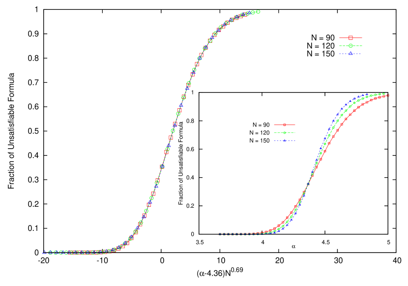
Figure 2: Scaled numerical data for $p=1/2$ for random $3$-SAT on a regular random graph. The inset shows the unscaled value of the fraction of unsatisfied formulae as a function of $\alpha$.

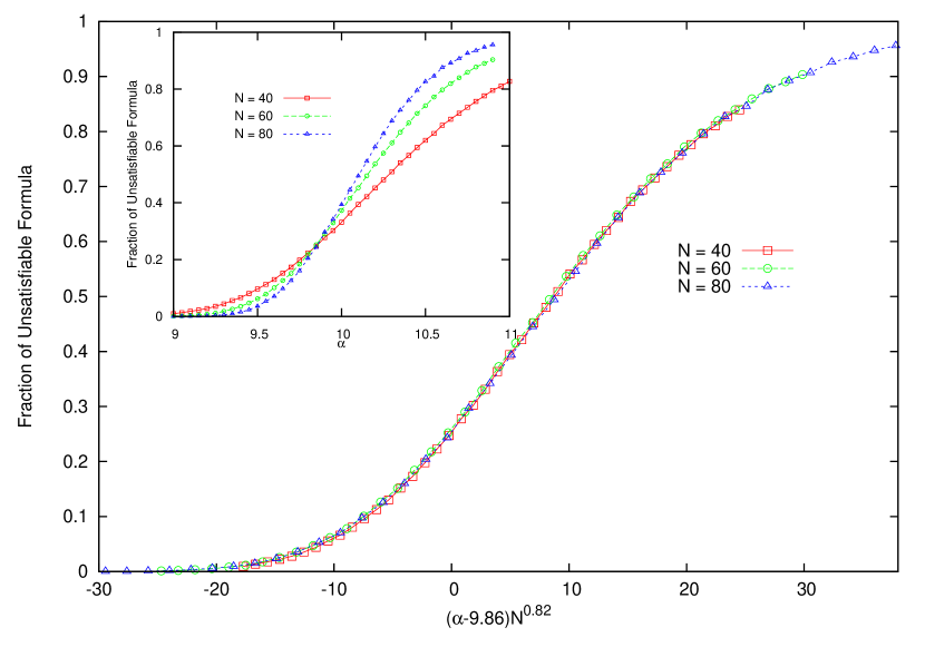
Figure 3: Scaled numerical data for $p=1/2$ for random $4$-SAT on a regular random graph. The inset shows the unscaled value of the fraction of unsatisfied formulas as a function of $\alpha$.

III Balanced K-SAT

Balancing literals adds a dependency between variables, that complicates the problem. In Balanced $K$-SAT each literal is constrained to occur negated or non-negated exactly half the time. This model was shown to have higher complexity than random $K$-SAT boufkhad . It is also a harder problem for standard SAT solvers as they depend on variable selection which exploits the difference in literal degrees. In the usually-studied version of the problem with $N$ nodes having an average degree $r$, the number of literals appearing with either sign is $Nr/2$. As mentioned earlier, apart from studying the above we also study a variant of the problem where the number of literals of one kind is $fNr$ while the number of the opposite kind is $(1-f)Nr$ for any $0<f<1$. For $f=1/2$, the problem is the usual one. For this case, bounds on the threshold have been derived in vish using the second moment method. For $K=3$ the problem has also been studied by Castellana and Zdeborová zdeborova using the cavity method.

III.1 Balanced regular $K$-SAT on a tree

Now besides, fixing the degree of variables to be $(d+1)$, we also fix the degree of the literals. Let a variable occur negated/non-negated exactly $(d+1)/2$ times. We define $q$ to be the integer value of $(d+1)/2$. We aim to write recursions for $Q_{n}$ as defined in the previous section. While the logic for writing these recursions is the same as before, the subtlety here is that, because of the balancing condition, whether a variable at depth $n$ is negated or not in the clause connecting it to depth $n+1$ is not independent of whether it is negated or not in the other clauses it participates in. Nevertheless, our method is easily modified to deal with this situation. For ease of presentation we use the terms ’downward’ and ’upward’ to denote a variable’s connections to clauses at lower and higher depths respectively. Also, since the balancing condition crucially depends on whether $d$ is even or odd, we first do these two cases separately before presenting a general formula valid for any value of $d$ (including non integer values).

III.1.1 When d is odd

Since each variable occurs in $d+1$ clauses, the only realizations that are allowed are when it is negated and not negated in exactly $(d+1)/2=q$ clauses. This leads to one literal occuring $q$ times and the other $q-1$ times amongst the downward clauses. The upward clause then contains the literal which appeared as a minority amongst the downward clauses. Since the two cases of whether the minority literal is a negation or a non-negation are entirely equivalent, it suffices to look at only one of these two cases.

We need now to consider two situations separately - when the minority literal is true or when the majority literal is true. In the former case, the variable is guaranteed to satisfy the upward clause while in the latter case, it is guaranteed to unsatisfy the upward clause.

The equations for $P_{n}(0)$, $P_{n}(1)$ and $Q_{n}$ can be written as before. They are:

$$P_{n+1}(0)=(1-(1-Q_{n}^{K-1})^{q})(1-(1-Q_{n}^{K-1})^{q-1})$$ (17)

$$P_{n+1,-}(1) = (1-(1-Q_{n}^{k-1})^{q})(1-Q_{n}^{k-1})^{q-1}$$ (18)

$$P_{n+1,+}(1) = (1-(1-Q_{n}^{k-1})^{q-1})(1-Q_{n}^{k-1})^{q}$$ (19)

and

$$P_{n+1}(1)=P_{n+1,-}(1)+P_{n+1,+}(1)$$ (20)

Here $P_{n+1,-}(1)$ denotes the probability of the majority literal being true and $P_{n+1,+}(1)$ denotes the probability of the minority literal being true. The equation for $Q_{n}$ is then

$$Q_{n+1}=\left(\frac{P_{n+1,-}(1)}{1-P_{n+1}(0)}\right)$$ (21)

A fixed point analysis of this equation exhibits a continuous transition for $K=2$ and a discontinuous transition for $K\geq 3$. For $K=2$ the transition occurs at $d=1$. For $K=3$ and $d=7$ the fixed point equation has only one trivial solution ($Q=0$), while at $d=9$ it has three solutions, suggesting a first order transition point in between these two values of $d$.

III.1.2 When d is even

In this case, its not possible to have exactly $(d+1)/2$ literals of one sign associated with every variable. Every variable has hence $d/2$ (or $q$) literals of one sign and $d/2+1$ (or $q+1$) literals of the opposite sign. Balancing is achieved by ensuring that for a graph of $N$ variables, exactly half the number of variables have, on average, $q$ literals of one sign while the other half have $q$ literals of the opposite sign.

As before, whether the minority number $q$ denotes negated or non-negated variables is equivalent and we need only consider one of these cases. For a given sign of $q$ literals we need to consider again two distinct cases: All $q$ of the minority literals occur amongst the downward clauses or $q-1$ of the minority literals occur amongst the downward clauses and one in the upward clause. The former possibility occurs with probability $q/(2q+1)$ and the latter with probability $(q+1)/(2q+1)$. The equation for $P_{n}(0)$ is now:

$$P_{n+1}(0)=(1-(1-Q_{n}^{K-1})^{q-1})(1-(1-Q_{n}^{K-1})^{q+1})\frac{q}{2q+1}+(1-(1-Q_{n}^{K-1})^{q})(1-(1-Q_{n}^{K-1})^{q})\frac{q+1}{2q+1}$$ (22)

The first term accounts for the case when all the majority literals occur amongst the downward clauses and the second term for the equivalent case when the minority variables all occur amongst the downward clauses. As before, for each of these two situations, the probability that the variable in question cannot take either value is that at least one of the clauses this variable satisfies as well at least one of the clauses that this variable unsatisfies are also unsatisfied by the other variables which participate in them.

Similarly, $Q_{n}$ is the probability (conditional on the node being able to take at least one value) that a node at level $n$ takes the one value that unsatisfies the upward clause. This happens when the node satisfies either the majority or minority literals which all occur amongst the downward clauses.

This gives:

$$Q_{n+1} = \frac{q}{2q+1}\left(\frac{(1-(1-Q_{n}^{K-1})^{q+1})(1-Q_{n}^{K-1})^{q-1}}{(1-P_{n+1}(0))}\right)$$ (23)

$$+ \frac{1+q}{2q+1}\left(\frac{(1-(1-Q_{n}^{K-1})^{q})(1-Q_{n}^{K-1})^{q}}{(1-P_{n+1}(0))}\right)$$ (24)

On solving for the fixed point, this equation indicates a continuous transition for $K=2$ between $d=0$ and $d=2$ and a first order transition for $K=3$ between $d=8$ and $d=10$.

III.1.3 For general d

Though the tree is defined for integer values of $d$, we can extend the above recursions to non-integer values. One way to do it is the folowing. For any arbitrary value of $d$, consider that a variable can occur negated in $q$ clauses a fraction $y$ of the times and in $q+1$ clauses a fraction $1-y$ of the times where $q$ is defined as before. The value $y=1/2$ corresponds to even $d$ while $y=1$ corresponds to odd $d$. So we have

$$yq+(1-y)(q+1)=\frac{d+1}{2}$$ (25)

Note that the actual degree of the nodes is always $2q+1$. So, for each variable, there is always one more of a literal of one sign over the other when $(d+1)/2$ is not an integer. The parameter $y$ ensures that on average the number of literals of either kind per node is always $(d+1)/2$, by fixing the fraction of nodes with one more negation over a non-negation or vice versa. This procedure works for any $d$, including non-integral values since all that is needed is to fix $y$ accordingly from the above equation.

The fixed point equation in this case for a general $y$ is exactly the same as Eq. 23 for the case $y=1/2$.

Hence we can perform a fixed point analysis of this equation for non-integer $d$. We get $d_{c}=1$ and hence $\alpha_{c}=(d_{c}+1)/2=1$ for $K=2$ and $d_{c}=8.65\pm 0.05$ for $K=3$ which gives $\alpha_{c}=(d_{c}+1)/3=3.23$.

III.1.4 f-balanced regular $K$- SAT

If instead of fixing the ratio of negated to non-negated to be $1/2$, we assume that it is some general fraction $f$, then again it is easy to write the fixed point recursion. For any general $f$, if $q$ is the integer value of $f(d+1)$, then we have to now consider two kinds of nodes: one for which the difference between the minority and majority literals is $d+1-q$ and the other for which the difference between the two is $d-q$. The value of $y$ fixes the fraction of these two kinds of nodes. The value $y=1-f$ corresponds to the case when $fd$ is an integer and the value $y=1$ corresponds to the case when $f(d+1)$ is an integer. For general $y$ we have,

$$yq+(1-y)(q+1)=f(d+1)$$ (26)

The equations for $P_{n}(0)$ is now:

$$P_{n+1}(0) = \left((1-F^{q-1}_{n,K})(1-F^{d+1-q}_{n,K})\frac{q}{d+1}+(1-F^{q}_{n,K})(1-F^{d-q}_{n,K})\frac{d+1-q}{d+1}\right)y$$

$$+ \left((1-F^{q}_{n,K})(1-F^{d-q}_{n,K})\frac{q+1}{d+1}+(1-F^{q+1}_{n,K})(1-F^{d-q-1}_{n,K})\frac{d-q}{d+1}\right)(1-y)$$

here we have defined $F_{n,K}=1-Q_{n}^{K-1}$ for ease of presentation.

As before to get the fixed point equation for $Q_{n}$, we need only consider the cases when the literal that is satisfied occurs entirely amongst the downward clauses.

$$Q_{n+1} = y\left(\frac{(d-q+1)(1-F^{q}_{n,K})F^{d-q}_{n,K}}{(d+1)(1-P_{n+1}(0))}+\frac{qF^{q-1}_{n,K}(1-F^{d+1-q}_{n,K}}{(d+1)(1-P_{n+1}(0))}\right)$$

$$+ (1-y)\left(\frac{(d-q)(1-F^{q+1}_{n,K})F^{d-q+1}_{n,K}}{(d+1)(1-P_{n+1}(0))}+\frac{(q+1)F^{q}_{n,K}(1-F^{d-q}_{n,K})}{(d+1)(1-P_{n+1}(0))}\right)$$

III.2 Comparison with random graph

Balancing the literals makes the problem more constrained. For a given distribution of degrees, $D=<r_{+}r_{-}>=f(1-f)<r^{2}>$ in the case when each literal is chosen with one sign $f$ times and the other sign $(1-f)$ times. Applying the theorem described in Section II.2 results in the following threshold equation for f-balanced $2$-SAT:

$$2f(1-f)<r^{2}>-<r>=0$$ (28)

Hence in the balanced literal case the threshold is sensitive to the underlying distribution through the second moment. For $f=1/2$ we have the lowest threshold and the equation in that case is :

$$<r^{2}>-2<r>=0$$ (29)

Interestingly this equation is exactly the same as the equation for the percolation threshold on a random graph with a given degree distribution molloy1 . As argued by Molloy et al molloy2 , the SAT threshold cannot be lower than the percolation threshold. This implies that the most constrained $2$-SAT problem for a given degree/variable distribution is the one where the literals are exactly balanced ($f=1/2$).

For balanced $2$-SAT on regular random graphs, $<r^{2}>=r^{2}$, and hence $\alpha_{c}=1/(4f(1-f)$. We have compared this with the threshold obtained from the fixed point analysis of Eq. LABEL:f-bal and it matches exactly. For example for $f=1/2$, we get $\alpha_{c}=1$.

We have also considered balanced $2$-SAT with poisson distributed degree on a random graph. Unlike the regular random $2$-SAT, the threshold here for any arbitrary degree distribution depends on its second moment. For balanced $2$-SAT with Poisson distributed degree on a random-graph, $<r^{2}>=<r>+<r>^{2}$. Substituting in Eq. 28 gives $<r_{c}>=(\frac{1}{2f(1-f)}-1)$ and hence $\alpha_{c}=1/(4f(1-f))-1/2$. This gives $\alpha_{c}=1/2$ for $f=1/2$. Note that this is also the percolation threshold for Erdös-Réyni random graphs. This suggests that the model with balanced literals and a Poisson degree distribution on a random graph has the lowest SAT-UNSAT threshold among all possible models for $K=2$.

For $K>2$, as in biased random K-SAT, the values obtained from the tree calculation seem to give a lower bound on the threshold value obtained numerically on regular random graphs (see Table 3). We have also simulated balanced SAT on random graphs for $K=3$ and $4$ for $f=1/2$. Figs. 4 and 5 plot the values of the fraction of unsatisfied formulas as a function of $\alpha$ for balanced $3$-SAT and $4$-SAT respectively, on a regular random graph. Figs. 6 and 7 show the same quantity for $3$-SAT and $4$-SAT on a random graph. Within numerical precision, the threshold on a random graph is lower than that on a regular random graph. As expected however, the difference deceases with increasing $K$.

The problem of $K=3$ balanced SAT on regular and random graphs was studied using belief propagation and survey propagation by Castellana and Zdeborovázdeborova . They find that on regular random graphs, survey propagation starts to converge towards a non-trivial fixed point for $r>9$. The corresponding value they find for random graphs is $\alpha>3.2$. Our calculations on a tree give a nontrivial fixed point at $d_{c}+1=9.65$, consistent with the results presented in zdeborova . This gives us $\alpha_{C}=3.23$ on a tree. Again this is very close to the $\alpha_{d}$ obtained in zdeborova using survey propagation for balanced SAT on random graphs.

Table 3: Comparison of threshold for balanced $K$-SAT on tree, regular random graph(RRG) and random graph(RG)(See also Figs. 4,5,6 and 7). The starred values of the threshold obtained using cooper in the table are exact.

$K$	Tree	RRG numerics	RG numerics
$2$	$1$	$1^{*}$	$1/2^{*}$
$3$	$3.23$	$3.5\pm 0.02$	$3.37\pm 0.02$
$4$	$7.163$	$8.69\pm 0.02$	$8.65\pm 0.02$

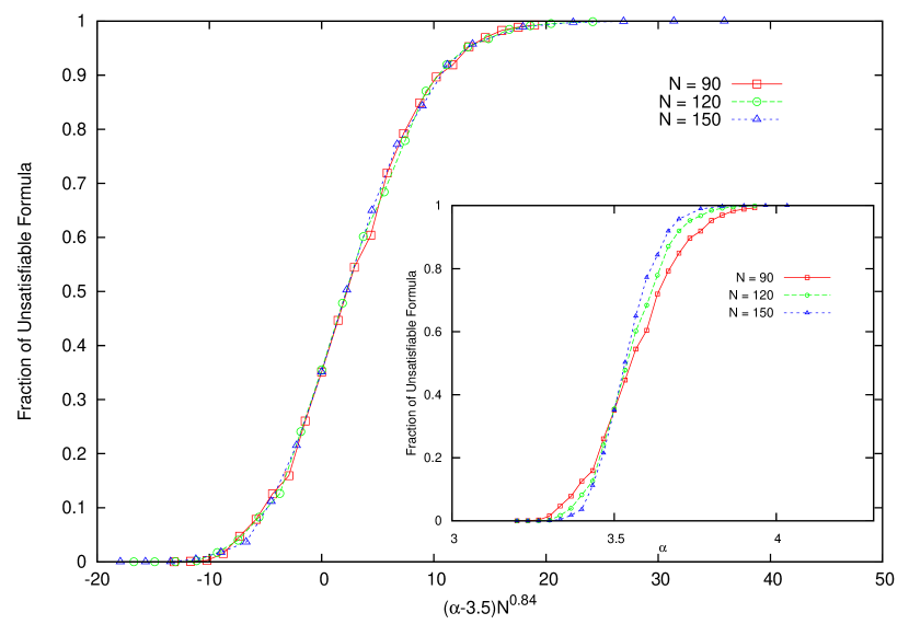
Figure 4: Scaled numerical data for $f=1/2$ balanced $3$-SAT on a regular random graph. The inset shows the unscaled value of the fraction of unsatisfied formulae as a function of $\alpha$.

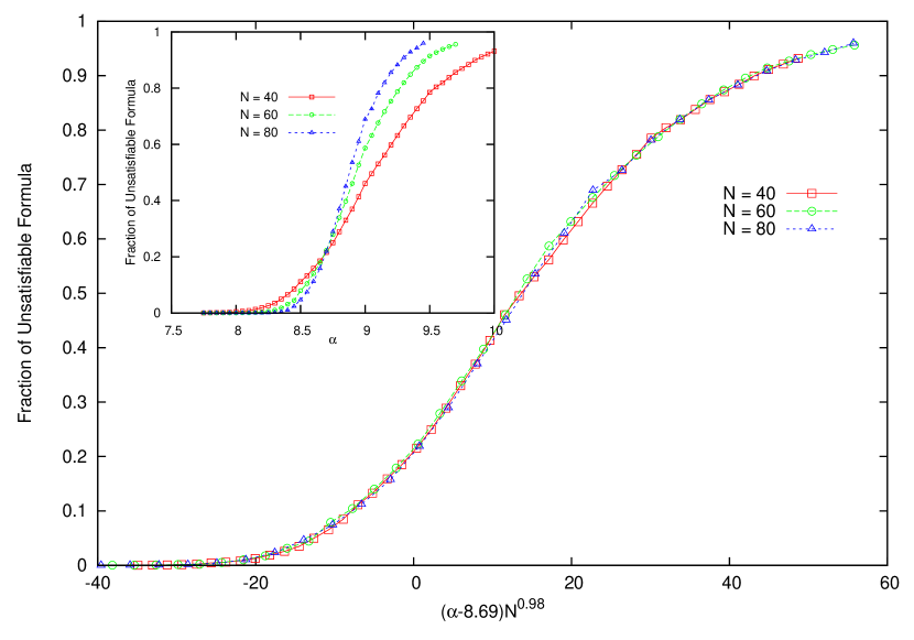
Figure 5: Scaled numerical data for $f=1/2$ balanced $4$-SAT on a regular random graph. The inset shows the unscaled value of the fraction of unsatisfied formulae as a function of $\alpha$.

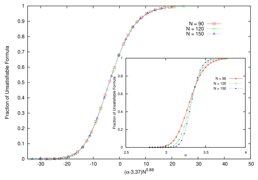
Figure 6: Scaled numerical data for $f=1/2$ balanced $3$-SAT on a random graph. The inset shows the unscaled value of the fraction of unsatisfied formulae as a function of $\alpha$.

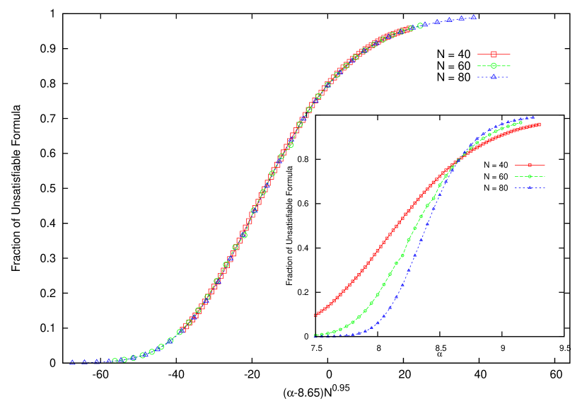
Figure 7: Scaled numerical data for $f=1/2$ balanced $4$-SAT on a random graph. The inset shows the unscaled value of the fraction of unsatisfied formulae as a function of $\alpha$.

IV Connection with Survey Propagation and Reconstruction

The recursions we developed in ss and in this paper are connected to the well-known problem of tree reconstruction. The reconstruction problem, as originally defined, is a broadcast model on a tree, such that information is sent from the root to the leaves, across edges which act as noisy channels. The problem then is whether we can recover information about the root from a knowledge of the configuration of the leaves. Apart from its intrinsic interest, it is also of interest for $K$-SAT because it has been shown that the recursions developed in the reconstruction context are exactly the same as obtained by other means (such as the replica or cavity methods) for the dynamical glass transition on a random graph mezard-montanari or the clustering transition for $K$ SAT (the value of $\alpha$ beyond which the solution-space is fragmented into different clusters).

In terms of reconstruction, these fixed point recursions are developed for the unconditional probability distribution at the root of the tree to have a certain ’bias’ ; namely, the fraction of boundary conditions (out of all boundary conditions that have a non-zero solution set), weigted by the total number of solutions these boundary conditions possess, that leads to the root taking the value $-1$ a certain number of times and the value $1$ a certain number of times.

The fixed point equations developed in ss and in this paper have three differences in comparison with the one developed in mezard-montanari ; bhatnagar-maneva . We look at a reduced quantity - if the root can take two values (no matter what the bias), we lump it together to call it $P_{n}(2)$ for a level $n$. The quantity of interest that we can now derive is a fixed point distribution for a single number, namely $Q_{n}\equiv P_{n}(1)/2(1-P_{n}(0))$. This makes our recursions similar in spirit to Survey propagation (SP) as we explain below.

Secondly and more importantly, $P_{n}(1)$, $P_{n}(2)$ etc give the fraction of realizations, at the root, which have a non-zero solution set and not the fraction of boundaries.

Thirdly, unlike in mezard-montanari ; bhatnagar-maneva , where boundary conditions are weigted by the number of solutions they lead to, we do not weight the realizations by the number of solutions they have. Rather, to get $P_{n}(2)$ for example, we weight each realization equally in which the root can take both values $1$ and $-1$.

To see the similarities with earlier approaches better, let us now define the probability space over boundary conditions instead of realizations. We now derive a recursion for the fraction of boundary conditions that fix the value unambiguously at the root (so that it is either $-1$ or $1$) at level $n$, given this quantity for level $n-1$. Only those boundary conditions that lead to solutions at level $n-1$ are permitted. Note, as mentioned earlier, this is different from tree reconstruction in that now each boundary is weighted equally and not by the number of solutions it leads to.

These equations are the same as those derived earlier in ss , since the constraints that lead to the recursions are the same (and are defined once we specify the model). The only difference is that, since we are working with a typical realization, the extra average over all realizations is no longer allowed. The equations are hence

$$P_{n+1}(0) = \left[1-\left(1-\left(\frac{P_{n}(1)}{2(1-P_{n}(0))}\right)^{K-1}\right)^{d_{1}}\right]\left[1-\left(1-\left(\frac{P_{n}(1)}{2(1-P_{n}(0))}\right)^{K-1}\right)^{d-d_{1}}\right]$$

$$P_{n+1}(1) = \left(1-\left(\frac{P_{n}(1)}{2(1-P_{n}(0))}\right)^{K-1}\right)^{d-d_{1}}+\left(1-\left(\frac{P_{n}(1)}{2(1-P_{n}(0))}\right)^{K-1}\right)^{d_{1}}-$$ (30)

$$2\left(1-\left(\frac{P_{n}(1)}{2(1-P_{n}(0))}\right)^{K-1}\right)^{d}$$

where $d_{1}$ is a particular realization of negations at the root. The factor of $2$ in the expression $P_{n}(1)/(2(1-P_{n}(0)))$ appears because if $P_{n}(1)$ is the total fraction of bc’s that determine the root (at level $n$) to be either $-1$ or $1$, then, because of symmetry, exactly half of these configurations will not satisfy the link to level $n+1$, no matter what this link is.

If we replace $P_{n}(1)/(2(1-P_{n}(0)))$ by $Q_{n}$ as before, and in addition replace $d_{1}$ by $~{}d/2$ to specify a typical realization, then we get the recursion

$$Q_{n+1}=\frac{\left[1-Q_{n}^{K-1}\right]^{d/2}-\left[1-Q_{n}^{K-1}\right]^{d}}{{2\left[1-Q_{n}^{K-1}\right]^{d/2}-\left[1-Q_{n}^{K-1}\right]^{d}}}$$ (31)

The fixed points for different $K$ obtained from the above equation are very close to the values obtained earlier in ss . Infact, in the above form, we can also relate Eq. 31 to the form of the recursions derived in reference mmz in their analysis of the SP algorithm. To see this, note that if we substitute $z=(1-Q^{K-1})^{d/2}$ in Eqn 31, we get the recursion

$$z=\left[1-\left(\frac{1-z}{2-z}\right)^{K-1}\right]^{d/2}$$ (32)

In the SP language, $Q^{K-1}$ is the same as the cavity bias survey and $z$ is the analog of the probability of receving no supporting (or impeding) warning. Eq. 32 is exactly the recursion obtained in mmz , from the SP equations, when the probability distribution over the cavity bias surveys is replaced by a delta function, hence ignoring the differences in the values of these surveys between different variables $i$ or different realizations.

In our case, we get the recursions quite simply and without any approximations, from the way we have set up the problem in terms of computing the fraction of solvable realizations. It is remarkable that these two different ways of thinking of the problem, one of which gives an estimate of the solvability transition and the other an estimate of the clustering transition, give the same recursions.

In another interesting analogy, the recursions in Eq. IV are also exactly in the spirit of the ’naive reconstruction’ algorithm mentioned by Semerjian semer where a connection is now made with the freezing transition.

In conclusion our main contribution in this paper is that we have been able to get the exact SAT-UNSAT threshold for a number of models of random $K$-sat on a $d$-ary tree. This threshold matches exactly with the threshold on a random graph for $K=2$ and is very close to the numerical estimate of the threshold for $K=3$. In addition the numbers we get are equal to the numbers obtained for the dynamical glass transition for higher $K$ mmz . The latter is a result of the fact that our equations though averaged over realizations, might equally well be thought of as an average over boundary conditions, and hence are connected to the analysis of the SP algorithm. However note that in our way of setting up the fixed point equations, we can directly make a connection with the solvability transition which, to our knowledge, has not been mentioned before in the context of a tree calculation. Usually the solvability transition is estimated via the complexity mmz , which is defined as the number of constrained clusters in a typical instance of the problem. The complexity is calculated using the cavity method - it becomes non-zero at $\alpha_{d}$ and reduces in value as $\alpha$ increases till it reaches $0$, which is the point conjectured to be the solvability transition. The values obtained by these means are very close to numerics for all values of $K$, unlike in our case. It would be interesting to understand whether any analog of the complexity can be formulated for the tree.

Our fixed point equations are for a reduced or coarse-grained probability distribution function, but for this simplified quantity, we are able to write down an equation in closed form. It would be very interesting to understand whether, in our formalism, the above is also possible for the full distribution, such as the distribution of the fraction of realizations (or boundary conditions) that the root takes the value $-1$ a fraction $\beta$ of the times and the value $1$ a fraction $1-\beta$ of the times. For either of these cases, weigting realizations by the number of solutions they possess is also an obvious generalization of the results presented here, which would be useful to investigate.

Also, as mentioned here, variations of the same recursions seem to have connections to the clustering transition mmz , the freezing transition semer , and the solvability transition ss . It would be useful to quantify this better, as a tree calculation being exact, would make it possibile to obtain precise bounds on these transitions.

Our study of the different cases of balancing literals and degrees leads to the conclusion that balancing literals makes the problem harder while balancing the degree actually makes the problem easier. Hence the hardest problem, from the point of view of having the lowest SAT-UNSAT threshold is the case of balanced literals with a poisson degree distribution. In this case, for $K=2$ the solvability threshold is also the percolation threshold for Erdös-Réyni random graphs, consistent with the conjecture that the satisfiability threshold on a graph cannot be lower than the percolation threshold on the same graph.

References

- (1) D. Mitchell, B. Selman and H. Levesque, Proc. 10th Nat. Conf. Artif. Intel., 459 (1992).
- (2) S. Kirkpatrick and B. Selman, Science 264, 1297 (1994).
- (3) V. Chvatal and B. Reed, 33rd FOCS, 620 (1992); A. Goerdt, J. Comput. System. Sci., 53, 469 (1996); W. Fernandez de la vega, Theoret. Comput. Sci. 265, 131 (2001).
- (4) D. Achlioptas, Theoret. Compt. Sci. 265, 159 (2001).
- (5) M. Mèzard, G. Parisi and R. Zecchina, Science 297, 812 (2002).
- (6) R. Monasson and R. Zecchina, Phys. Rev. Lett. 76, 3881(1996).
- (7) S. Mertens, M. Mèzard and R. Zecchina, Random Structures and Algorithms, 28, 340 (2006).
- (8) G. Biroli, R. Monasson and M. Weigt, Eur. Phys. J. B, 14, 551 (2000).
- (9) F. Krzakala, A. Montanari, F. Ricci-Tersenghi, G. Semerjian and L. Zdeborová, PNAS 104, 10318 (2007).
- (10) G. Semerjian, J. Stat. Phys, 130, 251 (2008).
- (11) L. Zdeborová and F. Krzakala, Phys. Rev. E, 76, 031131 (2007).
- (12) D. Achlioptas and A. Coja-Oghlan, Proc. 49th FOCS, 793 (2008).
- (13) M. Mèzard and A. Montanari, J. Stat. Phys. 124, 1317 (2006).
- (14) S. Krishnamurthy and Sumedha, J. Stat. Mech, P05009(2012).
- (15) A. Ramezanpour and S Moghimi-Araghi, Phys. Rev. E 71 066101(2005).
- (16) M. Castellana, L. Zdeborová,J. Stat. Mech. (2011) P03023.
- (17) R. J Baxter, Exactly solvable models in statistical mechanics, Academic Press.
- (18) P. D. Gujrati Phys. Rev. Lett. 53, 2453(1984).
- (19) C Cooper, A Frieze and G B Sorkin, Proceedings of the annual ACM-SIAM symposium on Discrete Algorithms,316-320(2002).
- (20) R J Jr Bayardo and J D Pchousek, Proc. AAAI (MOnte Park,CA:AAAI Press),157-162(2000).
- (21) Y. Boufkhad, O. Dubois, Y. Interian and B. Selman, J. of Autom. Reasoning, 35, 181 (2005).
- (22) V. Rathi, E. Aurell, L. K. Rasmussen and M. Skoglund, SAT 2010, 264 (2010).
- (23) M Molloy and B Reed, Random Structures and Algorithms 6:2-3, 161(1995).
- (24) M Molloy, Combinatorica 28 693-734 (2008).
- (25) N. Bhatnagar and E. Maneva,SIAM J. on Discreet Math., 25, 854 (2011).
- (26) A. Montanari, R. Restrepo and P. Tetali, SIAM Journal on Discrete Mathematics (2011).