The effect of defect layer on transmissivity and light field distribution in general function photonic crystals

Abstract

We have theoretically investigated a general function photonic crystals (GFPCs) with defect layer, and choose the line refractive index function for two mediums $A$ and $B$, and analyze the effect of defect layer’s position, refractive indexes and period numbers on the transmission intensity and the electric field distribution. We obtain some new characters that are different from the conventional PCs, which should be helpful in the design of photonic crystals.

PACS: 42.70.Qs, 78.20.Ci, 41.20.Jb
Keywords: General photonic crystals; Defect model; Transmissivity; Light field distribution;

1. Introduction

Photonic crystals (PC) are a new kind of materials which facilitate the control of the light [1]. PC exhibits Photonic Band Gaps (PBG) that forbids the radiation propagation in a specific range of frequencies [2-6]. The PBG forbids the radiation propagation in a specific range of frequencies. The existence of PBGs will lead to many interesting phenomena, e.g., modification of spontaneous emission [7-9] and photon localization [10]. Thus numerous applications of photonic crystals have been proposed in improving the performance of optoelectronic and microwave devices such as high-efficiency semiconductor lasers, right emitting diodes, wave guides, optical filters, high-Q resonators, antennas, frequency-selective surface, optical limiters and amplifiers [11-18]. In the past ten years has been developed an intensive effort to study and micro-fabricate PBG materials in one, two or three dimensions [19-21]. In Refs. [22-25], we have proposed a general function photonic crystals (GFPCs), which refractive index is a arbitrary function of space position. Unlike conventional photonic crystals (PCs), which structure grow from two materials, A and B, with different dielectric constants $\varepsilon_{A}$ and $\varepsilon_{B}$, and have obtained some results different from the conventional photonic crystals. In the paper, We have studied the general function photonic crystals (GFPCs) with defect layer, and choose the line refractive index function for two mediums $A$ and $B$. We obtain some results: (1) When the position of defect layer move behind in the GFPCs, or the refractive indexes of defect layer increase, the transmission intensity maximum of defect model decreases. (2) When the period number of GFPCs increase, the transmission intensity of defect model increase, and the defect model’s width of half height become narrow. (3) Both the defect layer and it’s position have the effects on the electric field. (4) In the structure $(BA)^{N}D(BA)^{N}$, when the period number $N$ increase, the relative intensity of electric field increase. (5) When the refractive indexes of defect layer ($n_{d}$) increase, the relative intensity of electric field was enhanced.

2. The light motion equation in general function photonic crystals

For the general function photonic crystals, the medium refractive index is a periodic function of the space position, which can be written as $n(z)$, $n(x,z)$ and $n(x,y,z)$ corresponding to one-dimensional, two-dimensional and three-dimensional function photonic crystals. In the following, we shall deduce the light motion equations of the one-dimensional general function photonic crystals, i.e., the refractive index function is $n=n(z)$, meanwhile motion path is on $xz$ plane. The incident light wave strikes plane interface point $A$, the curves $AB$ and $BC$ are the path of incident and reflected light respectively, and they are shown in FIG. 1.

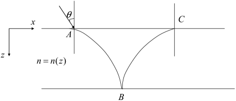
Figure 1: The motion path of light in the medium of refractive index $n(z)$.

The light motion equation can be obtained by Fermat principle, it is

$$\delta\int^{B}_{A}n(z)ds=0.$$ (1)

In the two-dimensional transmission space, the line element $ds$ is

$$ds=\sqrt{(dx)^{2}+(dz)^{2}}=\sqrt{1+\dot{z}^{2}}dx,$$ (2)

where $\dot{z}=\frac{dz}{dx}$, then Eq. (1) becomes

$$\delta\int^{B}_{A}n(z)\sqrt{1+(\dot{z})^{2}}dx=0.$$ (3)

The Eq. (3) change into

$$\int^{B}_{A}(\frac{\partial(n(z)\sqrt{1+\dot{z}^{2}})}{\partial z}\delta z+\frac{\partial(n(z)\sqrt{1+\dot{z}^{2}})}{\partial\dot{z}}\delta\dot{z})dx=0,$$ (4)

At the two end points $A$ and $B$, their variation is zero, i.e., $\delta z(A)=\delta z(B)=0$. For arbitrary variation $\delta z$, the Eq. (4) becomes

$$\frac{dn(z)}{dz}\sqrt{1+\dot{z}^{2}}-\frac{dn(z)}{dz}\dot{z}^{2}(1+\dot{z}^{2})^{-\frac{1}{2}}$$

$$-n(z)\frac{\ddot{z}\sqrt{1+\dot{z}^{2}}-\dot{z}^{2}\ddot{z}(1+\dot{z}^{2})^{-\frac{1}{2}}}{1+\dot{z}^{2}}=0,$$ (5)

simplify Eq. (5), we have

$$\frac{dn(z)}{n(z)}=\frac{\dot{z}d\dot{z}}{1+\dot{z}^{2}}.$$ (6)

The Eq. (6) is light motion equation in one-dimensional function photonic crystals.

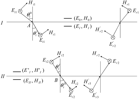
Figure 2: The light transmission and electric magnetic field distribution figure in FIG.1 medium.

3. The transfer matrix of one-dimensional general function photonic crystals

In this section, we should calculate the transfer matrix of one-dimensional general function photonic crystals. In fact, there is the reflection and refraction of light at a plane surface of two media with different dielectric properties. The dynamic properties of the electric field and magnetic field are contained in the boundary conditions: normal components of $D$ and $B$ are continuous; tangential components of $E$ and $H$ are continuous. We consider the electric field perpendicular to the plane of incidence, and the coordinate system and symbols as shown in FIG. 2.

On the two sides of interface I, the tangential components of electric field $E$ and magnetic field $H$ are continuous, there are

$$\left\{\begin{array}[]{ll}E_{0}=E_{I}=E_{t1}+E^{\prime}_{r2}\\ H_{0}=H_{I}=H_{t1}\cos\theta_{t}^{I}-H^{\prime}_{r2}\cos\theta_{t}^{I}.\end{array}\right.$$ (9)

On the two sides of interface II, the tangential components of electric field $E$ and magnetic field $H$ are continuous, and give

$$\left\{\begin{array}[]{ll}E_{II}=E^{\prime}_{I}=E_{i2}+E_{r2}\\ H_{II}=H^{\prime}_{I}=H_{i2}\cos\theta_{i}^{I}-H_{r2}\cos\theta_{i}^{I},\end{array}\right.$$ (12)

the electric field ${E_{t1}}$ is

$$E_{t1}=E_{t10}{e^{i(k_{x}x_{A}+k_{z}z)}|_{z=0}}=E_{t10}e^{i\frac{\omega}{c}n(0)\sin\theta_{t}^{I}x_{A}},$$ (13)

and the electric field ${E_{i2}}$ is

$$E_{i2} = E_{t10}{e^{i(k^{\prime}_{x}x_{B}+k^{\prime}_{z}z)}|_{z=b}}$$ (14)

$$= E_{t10}e^{i\frac{\omega}{c}n(b)(\sin\theta_{i}^{I}x_{B}+\cos\theta_{i}^{I}b)}.$$

Where $x_{A}$ and $x_{B}$ are $x$ component coordinates corresponding to point $A$ and point $B$. We should give the relation between $E_{i2}$ and $E_{t1}$. By integrating the two sides of Eq. (6), we can obtain the coordinate component $x_{B}$ of point $B$

$$\int^{n(z)}_{n(0)}\frac{dn(z)}{n(z)}=\int^{k_{z}}_{k_{0}}\frac{\dot{z}d\dot{z}}{1+\dot{z}^{2}},$$ (15)

to get

$$k_{z}^{2}=(1+k_{0}^{2})(\frac{n(z)}{n(0)})^{2}-1,$$ (16)

and

$$dx=\frac{dz}{\sqrt{(1+k_{0}^{2})(\frac{n(z)}{n(0)})^{2}-1}}.$$ (17)

where $k_{0}=\cot\theta_{t}^{I}$ and $k_{z}=\frac{dz}{dx}$ From Eq. (12), there is $n(z)>n(0)\sin\theta^{I}_{t}$. and the coordinate $x_{B}$ is

$$x_{B}=x_{A}+\int^{b}_{0}\frac{dz}{\sqrt{(1+k_{0}^{2})(\frac{n(z)}{n(0)})^{2}-1}},$$ (18)

where $b$ is the medium thickness of FIG. 1 and FIG. 2.
By substituting Eqs. (9) and (14)into (10), and using the equality

$$n(0)\sin\theta_{t}^{I}=n(b)\sin\theta_{i}^{I},$$ (19)

we have

$$E_{i2} = E_{t1}e^{i{\delta}_{b}},$$ (20)

where

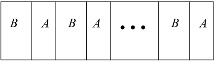
Figure 3: The structure $(BA)^{N}$ of the general function photonic crystals.

$$\delta_{b}=\frac{\omega}{c}n_{b}(b)(\cos\theta_{i}^{I}b+\sin\theta_{i}^{I}\int^{b}_{0}\frac{dz}{\sqrt{\frac{n_{b}^{2}(z)}{n_{0}^{2}\sin^{2}\theta_{i}^{0}}-1}}),$$ (21)

and similarly

$$E^{\prime}_{r2}=E_{r2}e^{i\delta_{b}}.$$ (22)

Substituting Eqs. (16) and (18) into (7) and (8), and using $H=\sqrt{\frac{\varepsilon_{0}}{\mu_{0}}}nE$, we obtain

$$\left(\begin{array}[]{c}E_{I}\\ H_{I}\\ \end{array}\right) = M_{B}\left(\begin{array}[]{c}E_{II}\\ H_{II}\\ \end{array}\right),$$ (27)

where

$$M_{B}=\left(\begin{array}[]{cc}\cos\delta_{b}&-\frac{i\sin\delta_{b}}{\sqrt{\frac{\varepsilon_{0}}{\mu_{0}}}n_{b}(b)\cos\theta_{i}^{I}}\\ -in_{b}(0)\sqrt{\frac{\varepsilon_{0}}{\mu_{o}}}\cos\theta_{t}^{I}\sin\delta_{b}&\frac{n_{b}(0)\cos\theta_{t}^{I}\cos\delta_{b}}{n_{b}(b)\cos\theta_{i}^{I}}\\ \end{array}\right),$$ (30)

The Eq. (20) is the transfer matrix $M$ in the medium of FIG. 1 and FIG. 2. By refraction law, we can obtain

$$\sin\theta^{I}_{t}=\frac{n_{0}}{n(0)}\sin\theta^{0}_{i},\cos\theta^{I}_{t}=\sqrt{1-\frac{n_{0}^{2}}{n^{2}(0)}\sin^{2}\theta^{I}_{t}},$$ (31)

where $n_{0}$ is air refractive index, and $n(0)=n(z)|_{z=0}$. Using Eqs. (15) and (21), we can calculate $\cos\theta_{i}^{I}$.

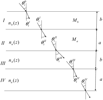
Figure 4: The two periods transmission figure of light in general function photonic crystals.

4. The transmissivity and light field distribution of one-dimensional general function photonic crystals

In section 3, we obtain the $M$ matrix of the half period. We know that the conventional photonic crystals is constituted by two different refractive index medium, and the refractive indexes are not continuous on the interface of the two mediums. We could devise the one-dimensional general function photonic crystals structure as follows: in the first half period, the refractive index distributing function of medium $B$ is $n_{b}(z)$. and in the second half period, the refractive index distributing function of medium $A$ is $n_{a}(z)$, corresponding thicknesses are $b$ and $a$, respectively. Their refractive indexes satisfy condition $n_{b}(b)\neq n_{a}(0)$, their structure are shown in FIG. 3, and FIG. 4. The Eq. (20) is the half period transfer matrix of medium $B$. Obviously, the half period transfer matrix of medium A is

$$M_{A}=\left(\begin{array}[]{cc}\cos\delta_{a}&-\frac{i\sin\delta_{a}}{\sqrt{\frac{\varepsilon_{0}}{\mu_{0}}}n_{a}(a)\cos\theta_{i}^{II}}\\ -in_{a}(0)\sqrt{\frac{\varepsilon_{0}}{\mu_{o}}}\cos\theta_{t}^{II}\sin\delta_{a}&\frac{n_{a}(0)\cos\theta_{t}^{II}\cos\delta_{a}}{n_{a}(a)\cos\theta_{i}^{II}}\\ \end{array}\right),$$ (34)

where

$$\delta_{a} = \frac{\omega}{c}n_{a}(a)[\cos\theta^{II}_{i}\cdot a$$ (35)

$$+\sin\theta^{II}_{i}\int^{a}_{0}\frac{dz}{\sqrt{\frac{n_{a}^{2}(z)}{n_{0}^{2}\sin^{2}\theta_{i}^{0}}-1}}],$$

$$\cos\theta^{II}_{t}=\sqrt{1-\frac{n_{0}^{2}}{n_{a}^{2}(0)}\sin^{2}\theta_{i}^{0}},$$ (36)

and

$$\sin\theta^{II}_{i}=\frac{n_{0}}{n_{a}(a)}\sin\theta_{i}^{0},$$ (37)

$$\cos\theta^{II}_{i}=\sqrt{1-\frac{n_{0}^{2}}{n_{a}^{2}(a)}\sin^{2}\theta_{i}^{0}}.$$ (38)

In one period, the transfer matrix $M$ is

$$M=M_{B}\cdot M_{A}$$

$$=\left(\begin{array}[]{cc}\cos\delta_{b}&\frac{-i\sin\delta_{b}}{\sqrt{\frac{\varepsilon_{0}}{\mu_{0}}}n_{b}(b)\cos\theta_{i}^{I}}\\ -in_{b}(0)\sqrt{\frac{\varepsilon_{0}}{\mu_{o}}}\cos\theta_{t}^{I}\sin\delta_{b}&\frac{n_{b}(0)\cos\theta_{t}^{I}\cos\delta_{b}}{n_{b}(b)\cos\theta_{i}^{I}}\\ \end{array}\right)$$ (41)

$$\left(\begin{array}[]{cc}\cos\delta_{a}&\frac{-i\sin\delta_{a}}{\sqrt{\frac{\varepsilon_{0}}{\mu_{0}}}n_{a}(a)\cos\theta_{i}^{II}}\\ -in_{a}(0)\sqrt{\frac{\varepsilon_{0}}{\mu_{o}}}\cos\theta_{t}^{II}\sin\delta_{a}&\frac{n_{a}(0)\cos\theta_{t}^{II}\cos\delta_{a}}{n_{a}(a)\cos\theta_{i}^{II}}\\ \end{array}\right).$$ (44)

The defect layer’s refractive index is constant $n_{d}$, its transfer matrix $M_{d}$ is

$$M_{d}=\left(\begin{array}[]{cc}\cos\delta_{d}&-\frac{i}{\eta_{d}}\sin\delta_{d}\\ -i\eta_{d}\sin\delta_{d}&\cos\delta_{d}\\ \end{array}\right),$$ (47)

where $\eta_{d}=\sqrt{\frac{\varepsilon_{0}}{\mu_{0}}}n_{d}$, $\delta_{d}=\frac{\omega}{c}n_{d}d$.
The form of the GFPCs transfer matrix $M$ is more complex than the conventional PCs. The angle $\theta_{t}^{I}$, $\theta_{i}^{I}$, $\theta_{t}^{II}$ and $\theta_{i}^{II}$ are shown in Fig. 4. The characteristic equation of GFPCs is

$$\left(\begin{array}[]{c}E_{1}\\ H_{1}\\ \end{array}\right) = M_{1}M_{2}\cdot\cdot\cdot M_{d}\cdot\cdot\cdot M_{N}\left(\begin{array}[]{c}E_{N+1}\\ H_{N+1}\\ \end{array}\right)$$ (52)

$$= M_{b}M_{a}M_{b}M_{a}\cdot\cdot\cdot M_{d}\cdot\cdot\cdot M_{b}M_{a}\left(\begin{array}[]{c}E_{N+1}\\ H_{N+1}\\ \end{array}\right)$$ (55)

$$= M\left(\begin{array}[]{c}E_{N+1}\\ H_{N+1}\\ \end{array}\right)=\left(\begin{array}[]{c c}A&B\\ C&D\\ \end{array}\right)\left(\begin{array}[]{c}E_{N+1}\\ H_{N+1}\\ \end{array}\right).$$ (62)

Where $N$ is the period number.

Figure 5: The refractive index of the general functions in a period.

Figure 6: The relation between transmissivity and frequency corresponding to the general function photonic crystals.

With the transfer matrix $M$ (Eq. (28)), we can obtain the transmission and reflection coefficient $t$ and $t$, and the transmissivity and reflectivity $T$ and $R$, they are

$$t=\frac{E_{tN+1}}{E_{i1}}=\frac{2\eta_{0}}{A\eta_{0}+B\eta_{0}\eta_{N+1}+C+D\eta_{N+1}},$$ (63)

$$r=\frac{E_{r1}}{E_{i1}}=\frac{A\eta_{0}+B\eta_{0}\eta_{N+1}-C-D\eta_{0}}{A\eta_{0}+B\eta_{0}\eta_{N+1}+C+D\eta_{0}},$$ (64)

and

$$T=t\cdot t^{*},$$ (65)

$$R=r\cdot r^{*}.$$ (66)

Where $\eta_{0}=\eta_{N+1}=\sqrt{\frac{\varepsilon_{0}}{\mu_{0}}}$. In the following, we give the electric field distribution of light in the one-dimensional GFPCs. The propagation figure of light in one-dimensional GFPCs is shown in FIG. 9. From Eq. (28), we have

$$\left(\begin{array}[]{c}E_{1}\\ H_{1}\\ \end{array}\right)=M_{1}(d_{1})M_{2}(d_{2})\cdot\cdot\cdot M_{d}(d)\cdot\cdot\cdot M_{N-1}(d_{N-1})$$ (69)

$$M_{N}(\Delta z_{N})\left(\begin{array}[]{c}E_{N}(d_{1}+d_{2}{\cdots}+d_{N-1}+\Delta z_{N})\\ H_{N}(d_{1}+d_{2}{\cdots}+d_{N-1}+\Delta z_{N})\\ \end{array}\right)$$ (72)

where $d_{1}$ and $d_{2}$ are the thickness of first and second period, respectively, $\Delta z_{N}$ is the propagation distance of light in the N-th period, $E_{1}$ and $H_{1}$ are the intensity of incident electric field and magnetic field, and $E_{N}(d_{1}+d_{2}{\cdots}+d_{N-1}+\Delta z_{N})$ and $H_{N}(d_{1}+d_{2}{\cdots}+d_{N-1}+\Delta z_{N})$ are the intensity of the N-th period electric field and magnetic field. The Eq. (34) can be written as

$$\left(\begin{array}[]{c}E_{N}(d_{1}+d_{2}{\cdots}+d_{N-1}+\Delta z_{N})\\ H_{N}(d_{1}+d_{2}{\cdots}+d_{N-1}+\Delta z_{N})\\ \end{array}\right)=M^{-1}_{N}(\Delta z_{N})$$ (75)

$$M^{-1}_{N-1}(d_{N-1})\cdot\cdot\cdot+M^{-1}(d)\cdot\cdot\cdot M^{-1}_{2}(d_{2})M^{-1}_{1}(d_{1})\left(\begin{array}[]{c}E_{1}\\ H_{1}\\ \end{array}\right)$$ (78)

$$\left(\begin{array}[]{cc}A(\Delta z_{N})&B(\Delta z_{N})\\ C(\Delta z_{N})&D(\Delta z_{N})\\ \end{array}\right)\left(\begin{array}[]{c}E_{1}\\ H_{1}\\ \end{array}\right),$$ (83)

the electric field $E_{1}$ and magnetic field $H_{1}$ can be written as

$$E_{1}=E_{i1}+E_{r1}=(1+r)E_{i1},$$ (84)

$$H_{1} = H_{i1}\cos\theta_{i}^{0}-H_{r1}\cos\theta_{i}^{0}$$ (85)

$$= \sqrt{\frac{\varepsilon_{0}}{\mu_{0}}}\cos\theta_{i}^{0}(1-r)E_{i1}.$$

From Eqs. (34)-(36), we can obtain the ratio of the electric field $E_{N}(d_{1}+d_{2}{\cdots}+d_{N-1}+\Delta z_{N})$ within the GFPCs to the incident electric field $E_{i1}$, it is

$$|\frac{E_{N}(d_{1}+d_{2}{\cdots}+d_{N-1}+\Delta z_{N})}{E_{i1}}|^{2}$$

$$=|A(\Delta z_{N})(1+r)+B(\Delta z_{N})\sqrt{\frac{\epsilon_{0}}{\mu_{0}}}\cos\theta_{i}^{0}(1-r)|^{2}.$$ (86)

5. Numerical result

In this section, we report our numerical results of transmissivity and light field distribution. We consider refractive indexes of the linearity functions in a period, it is

$$n_{b}(z)=n_{b}(0)+\frac{n_{b}(b)-n_{b}(0)}{b}z,\hskip 7.22743pt0\leq z\leq b,$$ (87)

$$n_{a}(z)=n_{a}(0)+\frac{n_{a}(a)-n_{a}(0)}{a}z,\hskip 7.22743pt0\leq z\leq a,$$ (88)

Eqs. (38) and (39) are the line refractive indexes distribution functions of two half period mediums $B$ and $A$. When the endpoint values $n_{b}(0)$, $n_{b}(b)$, $n_{a}(0)$ and $n_{a}(a)$ are all given, the line refractive index functions $n_{b}(z)$ and $n_{a}(z)$ are ascertained. The main parameters are: the half period thickness $b$ and $a$, the starting point refractive indexes $n_{b}(0)$ and $n_{a}(0)$, and end point refractive indexes $n_{b}(b)$ and $n_{a}(a)$, the optical thickness of the two mediums are equal, i.e., $n_{b}(0)b=n_{a}(0)a$, the incident angle $\theta_{i}^{0}=0$, the center frequency $\omega_{0}=1.215\times 10^{15}Hz$, the center wave length $\lambda_{0}=\frac{2\pi c}{\omega_{0}}$, the thickness $b=280nm$, $a=165nm$ and the period number $N=16$. we take $n_{b}(0)=1.38$, $n_{b}(b)=1.9$ for the medium $B$, and $n_{a}(0)=2.35$, $n_{a}(a)=2.6$ for the medium $A$, which are the up line function of refractive indexes, it is shown in FIG.5. By the refractive indexes function, we can calculate the transmissivity, we obtain the transmissivity distribution in FIG.6.

In FIG.7, we take $n_{b}(0)=n_{b}(b)=1.38$, $n_{a}(0)=n_{a}(a)=2.35$, i.e., the transmissivity of conventional photonic crystals. Compare FIG.6 with FIG.7, it can be found the results: (1) when the line function of refractive indexes is up, i.e., the GFPCs, the transmissivity can be far larger than $1$ ($T$ maximum is about $850$), while the maximum of transmissivity in conventional photonic crystals is $1$; (2) The number of band gaps in GFPCs are more than the conventional PCs.

Figure 7: The relation between transmissivity and frequency corresponding to the conventional photonic crystals.

In FIGs.8-10, we main discuss the relation between transmissivity and wave length corresponding to the GFPCs with defect layer, there is $n_{d}d=\frac{\lambda_{0}}{4}$. Base on the structure of GFPCs $(BA)^{16}$, we inset the defect layer at different position, which are shown in FIG.8(a-c). The structures are: (a)$(BA)^{8}D(BA)^{8}$, (b)$(BA)^{10}D(BA)^{6}$, (c)$(BA)^{12}D(BA)^{4}$, where $n_{d}=2$. We can see that when the position of defect layer is changed, the defect model become small.

Figure 8: Comparing the transmissivity of the GFPCs with different position of defect layer.

Figure 9: Comparing the transmissivity of the GFPCs ($(BA)^{N}D(BA)^{N}$) with different half period numbers (a) N=6 (b) N=7 (c) N=8.

Figure 10: Comparing the transmissivity of the GFPCs ($(BA)^{8}D(BA)^{8}$) with different refractive indexes of defect layer.

In FIG.9, we compare the transmissivity with different structure as $(BA)^{N}D(BA)^{N}$. In FIG.9(a-c), the half period number are: $N=6$, $N=7$ and $N=8$, where $n_{d}=2$. We can obtain the results: As the number of half period $N$ increase, for example, $N=6$, the maximum of defect model achieve $110$ (FIG.9(a)). When $N=7$, the intensity of defect model is about $250$ (FIG.9(b)). When $N$ increases up to $8$ (FIG.9(c)), the maximum of defect model nearly $400$, i.e., as the half period number $N$ increase, the maximum of defect model increase, the defect model’s width of half height become narrow and the transmissivity of the GFPCs also increase.

FIG.10 shows the transmissivity of the GFPCs ($(BA)^{8}D(BA)^{8}$) with different refractive indexes of defect layer. From FIG.10(a-c), $n_{d}$ are taken as: $1.5$, $2$ and $5$, respectively. Here, we notice that as the refractive indexes of defect layer increase, the intensity of defect model decrease, and the position of defect model become blue shift.

Figure 11: The light distribution in the conventional PCs. (a) without the defect layer($(BA)^{16}$), (b) with the defect layer ($(BA)^{8}D(BA)^{8}$). The bold line is the field distribution of defect layer.

Figure 12: The light distribution in the GFPCs. The structures are: (a) $(BA)^{16}$, (b) $(BA)^{8}D(BA)^{8}$, (c) $(BA)^{12}D(BA)^{4}$. The bold line is the field distribution of defect layer.

Figure 13: The light field distribution of the GFPCs ($(BA)^{N}D(BA)^{N}$)with different periodicity, (a) N=4, (b) N=6, (c) N=8. The bold line is the field distribution of defect layer.

FIGs.11-14 are the distribution of electric field. The transverse axis $z$ is propagation distance, and the longitudinal axis is the ratio of field intensity $E$ and incidence field intensity $E_{i1}$ square, i.e., $|E/E_{i1}|^{2}$.

FIG.11 is the distribution of electric field in conventional PCs. The structure of FIG.11(a-b) are $(BA)^{16}$ and $(BA)^{8}D(BA)^{8}$. The main parameters are the same as FIG.7, and the $n_{d}=2$, $n_{d}d=\frac{\lambda_{0}}{4}$. It can be found that the electric field was enhanced obviously when inserted the defect layer.

In the following, the main parameters are the same as FIG.6. In FIG.12, we study the effect of different structure of GFPCs on the distribution of light field. For FIG.12(a), the structure is $(BA)^{16}$, FIG.12(b) and FIG.12(c), the structure are $(BA)^{8}D(BA)^{8}$ and $(BA)^{12}D(BA)^{4}$, where $n_{d}=2$, $n_{d}d=\frac{\lambda_{0}}{4}$. Comparing FIG.12(a) with FIG.12(b), we found that when the defect layer is located in the middle of GFPCs, the electric field was weaken. While in FIG.12(c), the electric field was enhance. They are shown that both the defect layer and its’ position have the effects on the distribution of light field, and we can find the defect layer made the electric field local enhanced for the conventional PCs. While the defect layer made the electric field whole enhanced or decreased for the GFPCs.

In FIG.13, we shall consider the effect of half period number $N$ ($(BA)^{N}D(BA)^{N}$) on the electric field. Taken $N=4$, $N=6$ and $N=8$ corresponding to FIG.13(a-c). The results shown that when $N$ increase, the relative intensity of electric field heighten.

FIG.14 show the effect of different refractive indexes of defect layer ($n_{d}$) on the electric field. The structure is $(BA)^{8}D(BA)^{8}$. In FIG.14(a-c), $n_{d}$ are equal to $1.5$, $2$ and $3$, respectively. As we can see in FIG.14(a-c), when $n_{d}$ increase, the relative intensity of electric field was enhanced.

6. Conclusion

Figure 14: The light field distribution of the GFPCs ($(BA)^{8}D(BA)^{8}$)with different refractive indexes of defect layer. The bold line is the field distribution of defect layer.

In summary, We have theoretically investigated a new general function photonic crystals (GFPCs) with defect layer. Based on Fermat principle, we achieve the motion equations of light in one-dimensional general function photonic crystals, and calculate its transfer matrix. We choose the line refractive index function for two mediums $A$ and $B$, and obtain some results: (1) When the position of defect layer move behind in the GFPCs, or the refractive indexes of defect layer increase, the transmission intensity maximum of defect model decreases. (2) When the period number of GFPCs increase, the transmission intensity of defect model increase, and the defect model’s width of half height become narrow. (3) Both the defect layer and it’s position have the effects on the electric field. (4) In the structure $(BA)^{N}D(BA)^{N}$, when the period number $N$ increase, the relative intensity of electric field increase. (5) When the refractive indexes of defect layer ($n_{d}$) increase, the relative intensity of electric field was enhanced. Since the GFPCs has new character different from the conventional PCs, it should be helpful in the design of photonic crystals.

References

(1)
E. Yablonovitch, Phys. Rev. Lett. 58, 2059 C2062 (1987).
(2)
J. D. Joannopoulos, P. R. Villeneuve, and S. Fan, Nature 386,
143-149 (1997).
(3)
P. Russell, Photonic crystal fibers, Science 299, 358-362 (2003).
(4)
J. C. Knight, Photonic crystal fibres, Nature 424, 847-851 (2003).
(5)
A. F. Abouraddy, M. Bayindir, G. Benoit, S. D. Hart, K. Kuriki, N.
Orf, O. Shapira, F. Sorin, B. Temelkuranl, and Y. Fink, Nature
Photonics 6, 336-347 (2007).
(6)
S. John, Phys. Rev. Lett. 58, 2486-2489 (1987).
(7)
P. Nedel, X. Letartre, C. Seassal, A. Auff ves, L. Ferrier, E.
Drouard, A. Rahmani, and P. Viktorovitch., Optics Express. 19 5014 (2011).
(8)
C. Zinoni, B. Alloing, L. H. Li, F. Marsili, A. Fiore, L. Lunghi,
A. Gerardino, Yu. B. Vakhtomin, K. V. Smirnov, and G. N.
Gol’tsman., Appl. Phys. Lett. 91 031106 (2007).
(9)
S. G. Johnson and J. D. Joannopoulos., Optics Express. 8 173
(2001).
(10)
V. S. C. Manga Rao and S. Hughes., Phys. Rev. Lett. 99
193901 (2007).
(11)
G. Lecamp, P. Lalanne, and J. P. Hugonin., Phys. Rev. Lett. 99 023902 (2007).
(12)
V. S. C. Manga Rao and S. Hughes., Phys. Rev B 75 205437
(2007).
(13)
T. Lund-Hansen, S. Stobbe, B. Julsgaard, H. Thyrrestrup, T.
S nner, M. Kamp, A. Forchel, and P. Lodahl., Phys. Rev. Lett.
101 113903 (2008).
(14)
S. J. Dewhurst, D. Granados, D. J. P. Ellis, A. J. Bennett, R. B.
Patel, I. Farrer, D. Anderson, G. A. C. Jones, D. A. Ritchie, and
A. J. Shields., Appl. Phys. Lett. 96 031109 (2010).
(15)
K. Busch and S. John, Phys. Rev. Lett. 83, 967 (1999).
(16)
J-K. Yang, H. Noh, M. J. Rooks, G. S. Solomon, F. Vollmer and H.
Cao., Appl. Phys. Lett. 98, 241107 (2011)
(17)
R. Martinez-Sala, J. Sancho, J. V. Sanchez, V. Gomez, J. Llinares
and F. Meseguer, nature 378, 241 (1995).
(18)
D. Torrent, A. Hakansson, F. Cervera and J. Sanchez - Dehesa,
Phys. Rev. Lett. 96, 204302 (2006).
(19)
J. D. Joannopoulos, R. D. Meade, and J. N. Winn, Photonic
Crystals, Princeton University Press, Princeton (1995).
(20)
G. Guida, A. Lustrac and A. Priou, An introducion to Photonic Band
Gap (PBG) mate- rials, Progress In Electromagnetics Research,
PIER, Vol. 41, 1 C20 (2003).
(21)
K. Bush, S. Lolkes, R. B. Wehrspohn and H. Foll, Photonic
Crystals, Wiley, Berlin (2006).
(22)
Xiang-Yao Wu Bai-Jun Zhang Jing-Hai Yang, Xiao-Jing Liu Nuo
Ba Yi-Heng Wu and Qing-Cai Wang Physica E 43, 1694-1700
(2011).
(23)
Xiang-Yao Wu Bo-Jun Zhang Xiao-Jing Liu NuoBa Si-Qi
Zhang Jing Wang Physica E 44, 1223-1229 (2012).
(24)
Xiang-Yao Wu Bo-Jun Zhang Jing-Hai Yang Si-Qi Zhang Xiao-Jing
Liu Jing Wang, Nuo Ba, Zhong Hua and Xin-Guo Yin, Physica E 45, 166-172 (2012).
(25)
Xiang-Yao Wu Bo-Jun Zhang Xiao-Jing Liu Si-Qi Zhang Jing Wang,
Nuo Ba, Li Xiao and Hong Li Physica E 46, 133-138 (2012).