Screening Vector Field Modifications of General Relativity

Abstract

A screening mechanism for conformal vector-tensor modifications of general relativity is proposed. The conformal factor depends on the norm of the vector field and makes the field to vanish in high dense regions, whereas drives it to a non-null value in low density environments. Such process occurs due to a spontaneous symmetry breaking mechanism and gives rise to both the screening of fifth forces as well as Lorentz violations. The cosmology and local constraints are also computed.

Driven by cosmological observations, a plethora of theoretical models have been developed in the last decades to explain the evolution and composition of the Universe. Those models generally rely either on modifications of General Relativity (GR) or on the introduction of new exotic components in the Universe [1]. Often there is a mapping between the two approaches. For instance, $f(R)$ theories [2, 3], can be mapped via a conformal transformation into an interacting scalar field in Einstein’s gravity. In this new frame, the matter fields still feel the effects of the modified gravitational interaction because the scalar field couples to them. This gives rise to a fifth force which is tightly constrained by local gravity tests. Therefore, a general feature of novel theories to explain the nature of dark energy or dark matter, is that they modify general relativity at astrophysical scales, but are bound to recover GR at small scales via a screening mechanism.

Several screening mechanisms have been proposed in the literature: in the chameleon [4], the extra scalar degree of freedom becomes more massive in regions of high densities so that its range of interaction becomes very short and the fifth force is hidden from local gravity experiments (the existence of this mechanism in $f(R)$ theories was also shown in [5]); the symmetron mechanism [6] relies on an environmental-dependent potential, i.e., for low densities the potential has two minima so the field acquires a non-vanishing value, whereas for high enough densities the potential has only one minimum placed at the origin so that the scalar field vanishes; the Vainhstein mechanism [7] is based on kinetic self-interactions to hide the field on small scales. Recently, a mechanism to screen scalar fields via disformal couplings was proposed [8].

All the screening mechanisms in the literature have been developed for scalar degrees of freedom. Presently, there is no screening mechanism for vector-tensor modifications of GR, although chameleonic gauged B-L bosons have been discussed in [9]. However, higher spin fields are abundant in novel high energy physics theories, and have been explored in several cosmological and particle physics contexts. In fact, they have been proposed as candidates for Lorentz violation signatures, dark energy, dark matter, inflation or as generators of curvature perturbations [1, 10, 11, 12, 13, 14, 15, 16, 17]. If such fields exist, they also modify gravity and a screening mechanism is required by local gravity tests.

In this Letter, we propose a screening mechanism for vector-tensor gravity theories, in which the vector field hides its effects on small scales while producing relevant cosmological signatures.

We shall consider the simplest action to show this mechanism at work, which is that of a massive vector field with a gauge fixing term

$$S=\int{\rm d}^{4}x\sqrt{-g}\left[-\frac{R}{16\pi G}-\frac{1}{4}F^{2}-\frac{1}{2}(\nabla_{\mu}A^{\mu})^{2}-\frac{M^{2}}{2}A^{2}\right]+\int{\rm d}^{4}x{\mathcal{L}}_{m}[\tilde{g}_{\mu\nu},\psi],$$ (1)

where $R$ is the Ricci scalar constructed from the Levi-Civita connection of the metric $g_{\mu\nu}$, $F^{2}=g^{\mu\alpha}g^{\nu\beta}F_{\mu\nu}F_{\alpha\beta}$ with $F_{\mu\nu}=\partial_{\mu}A_{\nu}-\partial_{\nu}A_{\mu}$ and ${\mathcal{L}}_{m}$ is the Lagrangian for the matter fields, which couple to gravity through $\tilde{g}_{\mu\nu}$ given by

$$\tilde{g}_{\mu\nu}=B^{2}(A^{2})g_{\mu\nu},$$ (2)

with $A^{2}=g^{\mu\nu}A_{\mu}A_{\nu}$. Notice that, as usual with conformal transformations, this relation guarantees that both metrics lead to the same causal structure. In this Letter, we shall assume the particular case where the conformal factor is given by $B^{2}(A^{2})=e^{2\beta A^{2}/M_{p}^{2}}$.

The action (1) reduces to the Stueckelberg action for a massive vector field [18] in flat spacetime and when the vector field is much smaller than the Planck mass (see the Appendix). As in that scenario, one would also need to introduce the Stueckelberg field to compensate for the ghostly degree of freedom $A_{0}$ and, then, the theory can be quantised with a bounded hamiltonian following standard methods, in which one works with negative norm states in a restricted Hilbert space. Here, we will focus on the screening mechanism for the physical spatial components so that we have neglected the Stueckelberg field. In addition, we will show explicitly that the temporal component remains negligible in all the considered situations so that our results do not rely on its presence. Even though this does not prove the complete theoretical consistency of the full theory in an arbitrary background spacetime, we have chosen our action as a proof of concept of a working screening mechanism for a vector field.

The vector field equations of motion derived from the action (1) can be written as

$$\Box A_{\mu}=R_{\mu}{{}^{\nu}}A_{\nu}+\left(M^{2}+\frac{2\beta}{M_{p}^{2}}\tilde{g}^{\alpha\beta}\tilde{T}_{\alpha\beta}e^{4\beta A^{2}/M_{p}^{2}}\right)A_{\mu},$$ (3)

where $\tilde{T}_{\alpha\beta}\equiv\frac{2}{\sqrt{-\tilde{g}}}\frac{\delta{\mathcal{L}}_{m}}{\delta\tilde{g}^{\alpha\beta}}$. This energy-momentum tensor is not conserved under the covariant derivative associated to the Levi-Civita connection generated by the spacetime metric $g_{\alpha\beta}$, i.e., $\nabla_{\mu}\tilde{T}^{\mu\nu}\neq 0$. However, it is conserved under the covariant derivative associated to $\tilde{g}_{\mu\nu}$ so that $\tilde{\nabla}_{\mu}\tilde{T}^{\mu\nu}=0$. In other words, particles will follow the geodesics of the metric $\tilde{g}_{\mu\nu}$ and not those of $g_{\mu\nu}$. Notice that for the conformal coupling not to be trivial, it is necessary to have a dynamical norm for the vector field. Hence, this screening mechanism is not applicable to aether theories in which the norm of the vector field is fixed by means of a Lagrange multiplier [19].

Since we have two conformally related metrics, one could try to go to a Jordan frame in which matter is minimally coupled to the metric, and gravity would be described by a vector-tensor theory. In order to do that, it is necessary to invert (2). However, unlike in the scalar field case, the inverted relation is not simply $g_{\mu\nu}=B^{-2}(A^{2})\tilde{g}_{\mu\nu}$ because the argument of $B$ still depends on the metric $g_{\mu\nu}$. The main difficulty to invert this relation will be to solve the equation $\tilde{A}^{2}\equiv\tilde{g}_{\mu\nu}A^{\mu}A^{\nu}=B^{2}(A^{2})A^{2}$ for $A^{2}$ in terms of $\tilde{A}^{2}$. This equation will give rise, in general, to several branches that can lead to different theories in the Jordan frame. This can be useful, for instance, to constrain the vector field to be either timelike or spacelike in such a frame without having to introduce a Lagrange multiplier and, therefore, without reducing the number of degrees of freedom. We shall not pursue the consequences of going to the Jordan frame any further here (see however [20]). Let us simply mention that, in our case, the inversion of the conformal relation is given by $g_{\mu\nu}=e^{-W(2\beta\tilde{A}^{2})}\tilde{g}_{\mu\nu}$, being $W(x)$ the Lambert function.

In the case of a conformal coupling depending on a scalar field $\phi$, one finds $T_{\mu\nu}=B^{2}(\phi)\tilde{T}_{\mu\nu}$, where $T_{\mu\nu}\equiv\frac{2}{\sqrt{-g}}\frac{\delta{\mathcal{L}}_{m}}{\delta g^{\alpha\beta}}$ is the source of Einstein’s equations. However, in the case of our conformal factor depending on the vector field, we obtain

$$T_{\mu\nu}=B^{2}(A^{2})\left[\tilde{T}_{\mu\nu}-2B(A^{2})B^{\prime}(A^{2})\tilde{T}A_{\mu}A_{\nu}\right],$$ (4)

where a new term arises because the conformal factor $B^{2}(A^{2})$ depends itself on the metric. Notice that, since the additional term is proportional to the trace of $\tilde{T}_{\mu\nu}$, it disappears for a radiation-like component. Thus, in the cosmological evolution, it can only be important when the matter component is relevant and, indeed, it is a potential source of a large scale anisotropic stress. Nevertheless, this is not necessarily the case, since a vector field with a potential can yield an isotropic averaged energy-momentum tensor if it oscillates fast as compared to the Hubble expansion rate [21]

In order to understand the screening mechanism at small scales, we consider the vector field in a Minkowski spacetime and the matter field consisting of a pressureless fluid, i.e., $\tilde{g}^{\alpha\beta}\tilde{T}_{\alpha\beta}\simeq\tilde{\rho}$. As usual with conformal couplings, it is more convenient to use $\rho\equiv e^{3\beta A^{2}/M_{p}^{2}}\tilde{\rho}$, which does not depend on $A_{\mu}$ [4, 6]. The field equations (3) can then be written as

$$\Box A_{\mu}=\left(M^{2}+\frac{2\beta\rho}{M_{p}^{2}}e^{\beta(A_{0}^{2}-\vec{A}^{2})/M_{p}^{2}}\right)A_{\mu}.$$ (5)

We can interpret these field equations as those for a set of four scalar fields with an effective interaction that couples all four components. Even though this interaction cannot be written in terms of an effective potential as it is done in the scalar field case, the critical points can nevertheless be easily obtained

$$A_{\mu}=0,\;\;\;\;\;\bar{A}^{2}\equiv A_{0}^{2}-\vec{A}^{2}=\frac{M_{p}^{2}}{\beta}\log\frac{-M^{2}M_{p}^{2}}{2\beta\rho}.$$ (6)

The first critical point corresponds to a Lorentz invariant vacuum and always exists, whereas in the second one the field acquires a non-vanishing value, thus breaking Lorentz symmetry, and only exists if $M^{2}$ and $\beta$ have opposite signs. Moreover, for the second critical point, we find that in regions of high density, the vector field is spacelike (timelike) for $\beta$ negative (positive). In this Letter, we focus on the case with $\beta<0$ so that a spacelike vector field is screened and, thus, also Lorentz violations will be screened. In such a case, we can assume that $A_{0}\ll A_{i}$ so that the vector field is always space-like. This assumption is proved below to be consistent throughout the whole evolution, so that the vector field does not change from space-like to time-like. In such a case, the equations can be approximated by

$$\Box A_{\mu}=\left(M^{2}+\frac{2\beta\rho}{M_{p}^{2}}e^{-\beta\vec{A}^{2}/M_{p}^{2}}\right)A_{\mu}.$$ (7)

Thus, we can now define the following effective potential for the spatial components

$$V_{\rm eff}(\vec{A}^{2})=-\frac{1}{2}M^{2}\vec{A}^{2}+\rho e^{-\beta\vec{A}^{2}/M_{p}^{2}}.$$ (8)

The mass matrix at the critical point with $\vec{A}=0$ is $M_{ij}=m_{0}^{2}\delta_{ij}$ with

$$m_{0}^{2}=-M^{2}\left(1+\frac{2\beta\rho}{M^{2}M_{p}^{2}}\right).$$ (9)

Hence, in regions of high density, the effective mass is $m_{0}^{2}\simeq-2\beta\rho/M_{p}^{2}$ (which is positive for $\beta<0$) and the VEV of the field vanishes. However, in low dense regions, we have $m_{0}^{2}\simeq-M^{2}<0$ and the modes become tachyonic. For the second critical point, the masses given by the eigenvalues of the mass matrix are

$$m_{1}^{2}=m_{2}^{2}=0,\;\;\;\;\;m_{3}^{2}=2M^{2}\log\left[-\frac{M^{2}M_{p}^{2}}{2\beta\rho}\right].$$ (10)

This result was expected since the effective potential (8) exhibits an $O(3)$ symmetry that is spontaneously broken to $O(2)$ in the minimum of the effective potential, where the vector field spontaneously acquires a given value and points along one determined direction. This implies that one massive mode and two massless modes corresponding to the unbroken symmetries arise. Since the critical point only exists for $\log\left[-\frac{M^{2}M_{p}^{2}}{2\beta\rho}\right]>0$, the massive mode is always non-tachyonic.

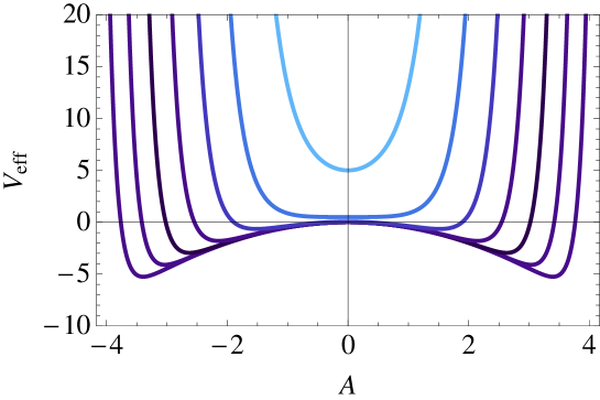
Figure 1: In this plot we show the effective potential given in (8) as a function of the modulus of the spatial components $|\vec{A}|\equiv A$ for different values of the energy density $\rho$. We can see how the effective potential exhibits the symmetry breaking explained in the main text when the density is low enough. Notice that at the minimum with $A\neq 0$, the direction of the VEV is only spontaneously acquired so that we still have the $O(2)$ symmetry corresponding to rotations around the direction determined by the VEV of $\vec{A}$.

The effective potential thus, exhibits a symmetry breaking mechanism when going from high to low densities (see Figure 1). At very high densities ($|2\beta\rho|\gg|M^{2}M_{p}^{2}|$), the effective potential has only one critical point located at the origin so that the vector field has a vanishing VEV and a positive mass $m_{0}^{2}\simeq\frac{2|\beta|\rho}{M^{2}M_{p}^{2}}$. On the other hand, when the density is low enough ($|2\beta\rho|\ll|M^{2}M_{p}^{2}|$), the critical point at the origin becomes tachyonic and the field runs away from it. However, the conformal coupling stabilises this tachyonic evolution and another set of critical points appear. In the new vacuum corresponding to the effective potential after the symmetry breaking, we have two massless modes plus a massive mode with mass $m_{3}^{2}$ given in (10).

The difference of our screening mechanism with respect to the symmetron is that, in the symmetron, the stabilisation of the tachyonic mode after the symmetry breaking is done by the $\phi^{4}$-term of the potential, whereas in our case the stabilisation comes from the exponential term of the conformal coupling. The fact that the stabilisation is done by an exponential instead of a quartic term is the reason why our screening process is more efficient after the symmetry breaking than in the original symmetron, although this could be very straightforwardly adapted for the symmetron.

The aforementioned critical points for the effective potential are the key for the screening mechanism: provided that $-M^{2}M_{p}^{2}\ll{2\beta\rho_{\rm local}}$ for the local density in the Solar System or our galaxy, the VEV of the vector field is zero. The leading order of the interaction of the vector field with the matter fields is $\beta A_{\rm VEV}^{\mu}\delta A_{\mu}T/M_{p}^{2}$ so that it decouples from matter in high density environments. When the vector field acquires a non-vanishing VEV, the strength of the interaction is set by $\beta A_{\rm VEV}^{\mu}/M_{p}^{2}$ so if we want this interaction to be of the same order as that of gravity, we need, at least, $\beta A_{\rm VEV}^{\mu}\sim M_{p}$. This condition is indeed fulfilled when the symmetry is broken and the field acquires the VEV given in (6), since the condition for the symmetry breaking is precisely $-\frac{M^{2}M_{p}^{2}}{2\beta\rho}\mathrel{\mathop{\kern 0.0pt\hbox to0.0pt{\raise 0.86108pt\hbox{$>$}\hss}}\lower 3.87495pt\hbox{\kern-1.90002pt$\sim$}}1$. It is also interesting to note that due to the conformal invariance of electromagnetism in 4 dimensions, photons do not couple to the vector field because of the tracelessness of its energy-momentum tensor. Finally, we should stress the fact that the interaction is direction dependent and only the component of the vector field parallel to its VEV couples to matter.

Another interesting feature of this mechanism is that, after the symmetry breaking takes place, we have a non-vanishing VEV for the vector field, so there is also a spontaneous breaking of Lorentz symmetry when going from high to low density regions. This represents a distinctive feature with respect to screening mechanisms for scalar fields. In fact, this mechanism can be regarded not only as a way to screen the fifth force mediated by the vector field, but also as a mechanism to screen Lorentz violations or, in other words, as a mechanism to dynamically restore Lorentz invariance in high density regions, while being broken in low density environments. Screening of Lorentz violating interactions has also been explored in [22] in the context of modified gravity theories with a scalar field $\phi$. In that case, the Lorentz violating coupling is through a coupling term $\partial_{\mu}\phi\partial_{\nu}\phi T^{\mu\nu}$ so that a direction dependent interaction appears when there is a background with non-vanishing gradients of the scalar field.

The local bounds on the theory can be computed by calculating the field profile near a static and spherically symmetric object. The field equations read

$$A_{0}^{\prime\prime}+\frac{2}{r}A_{0}^{\prime}=-\left[M^{2}+2\frac{\rho\beta}{M_{p}^{2}}e^{\beta A^{2}/M_{p}^{2}}\right]A_{0}$$ (11)

$$A_{z}^{\prime\prime}+\frac{2}{r}A_{z}^{\prime}=-\left[M^{2}+2\frac{\rho\beta}{M_{p}^{2}}e^{\beta A^{2}/M_{p}^{2}}\right]A_{z}.$$ (12)

To obtain the profile, we shall solve these equations outside and inside a spherical object. In the outer region, we assume that we are in the phase of symmetry breaking so that we will expand the equations to linearize them around the corresponding critical point. In such a case, the equations for the perturbations of the field with respect to their values at the fixed point are

$$\delta A_{0}^{\prime\prime}+\frac{2}{r}\delta A_{0}^{\prime}=\frac{2\beta M^{2}\bar{A}_{0}}{M_{p}^{2}}\left(\bar{A}_{0}\delta A_{0}-\bar{A}_{z}\delta A_{z}\right)$$ (13)

$$\delta A_{z}^{\prime\prime}+\frac{2}{r}\delta A_{z}^{\prime}=\frac{2\beta M^{2}\bar{A}_{z}}{M_{p}^{2}}\left(\bar{A}_{0}\delta A_{0}-\bar{A}_{z}\delta A_{z}\right)$$ (14)

where $\delta A_{0}\equiv A_{0}-\bar{A}_{0}$, $\delta A_{z}\equiv A_{z}-\bar{A}_{z}$ and $\bar{A}_{0}$, $\bar{A}_{z}$ are the asymptotic values. Now, as we commented above, we can assume that $\bar{A}_{0}\ll\bar{A_{z}}$ because the vector field is spacelike at the critical point. Then, assuming that the perturbations on both components are of the same order, we can further approximate the above equations to obtain

$$\delta A_{0}^{\prime\prime}+\frac{2}{r}\delta A_{0}^{\prime}\simeq m_{3}^{2}\frac{\bar{A}_{0}}{\bar{A}_{z}}\delta A_{z},$$ (15)

$$\delta A_{z}^{\prime\prime}+\frac{2}{r}\delta A_{z}^{\prime}\simeq m_{3}^{2}\delta A_{z}.$$ (16)

From these equations we can see that the source term for $\delta A_{0}$ is determined by $\delta A_{z}$ so that its profile will follow that of $\delta A_{z}$. Thus, since its asymptotic (cosmological) value $\bar{A}_{0}$ is assumed to be smaller than $\bar{A}_{z}$, it will remain smaller for all $r$. It is important to notice that both components satisfy the same equation inside the object, so that this remains true also in the inner region.

The obtained equations look similar to those in [6] so we can proceed in a similar manner to obtain the solutions inside and outside the object. The corresponding solutions for an object of density $\rho_{R}$ and size $R$ and with the boundary conditions $A^{\prime}_{z}(0)=0$ and $A(r\rightarrow\infty)\rightarrow\tilde{A}$, being $\tilde{A}$ the cosmological value, can be written as follows:

$$A_{z}^{\rm in}=B\frac{R}{r}\sinh\left[\frac{r}{R}\sqrt{\alpha^{2}-\mu^{2}}\right],$$ (17)

$$A_{z}^{\rm out}=C\frac{R}{r}e^{-m_{3}r}+\bar{A}_{z}$$

where $\alpha^{2}\equiv-2\beta\rho_{R}R^{2}/M_{p}^{2}$ and $\mu^{2}\equiv M^{2}R^{2}$ are dimensionless parameters. The mass $m_{3}$ is the one given in (10). It is important to notice that in the expression for $m_{3}$ we need to use the cosmological density and not $\rho_{R}$. On the other hand, we focus on the massive mode because the massless modes are less constraining. Finally, the constants $B$ and $C$ are obtained so that both solutions (and their first derivatives) match at $r=R$. In Figure 2 we show the profile corresponding to the above solution where we see the analogue of the thin-shell effect and how the field profile goes to zero very rapidly inside the object.

The force acting on a test particle due to the vector field is given by the gradient of the conformal factor $|\vec{F}|={\rm d}\ln B/{\rm d}r$, as obtained from the geodesic equations. We should notice here that, unlike in the scalar field case, the full expression for the fifth force actually depends on the gravitational potential because $B(A^{2})$ depends on the metric. If we assume the weak field limit with $g_{\mu\nu}=\eta_{\mu\nu}+h_{\mu\nu}$ where $|h_{\mu\nu}|\ll 1$, then the fifth force is given by

$$|\vec{F}| = \frac{\beta}{M_{p}^{2}}\left[2\Big{(}\eta^{\mu\nu}-h^{\mu\nu}\Big{)}A_{\mu}\frac{{\rm d}A_{\nu}}{{\rm d}r}-\frac{{\rm d}h^{\mu\nu}}{{\rm d}r}A_{\mu}A_{\nu}\right]$$

$$\simeq \frac{2\beta}{M_{p}^{2}}\left[A_{0}\frac{{\rm d}A_{0}}{{\rm d}r}-\vec{A}\cdot\frac{{\rm d}\vec{A}}{{\rm d}r}-\frac{1}{2}\frac{{\rm d}h^{\mu\nu}}{{\rm d}r}A_{\mu}A_{\nu}\right].$$

The last term in the bracket is proportional to the usual gravitational force given by the gradient of the gravitational potential so that it can be seen as a modification of Newton’s constant. Thus, the leading term of the fifth force gives a term proportional to the value of the field and its gradient and it also modifies the effective Newton’s constant. However, the effects are negligible inside the galaxy, since there the value of the field drops dramatically and we have a thin-shell effect (see Figure 2).

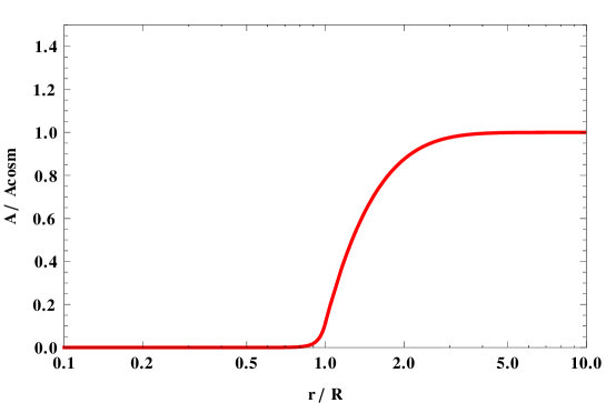
Figure 2: The field profile inside and outside the galaxy: the field goes to zero inside the galaxy whereas it tends to a non-vanishing (cosmological) value outside. Thus, inside the galaxy, the fifth force is screened and Lorentz symmetry is restored. As explained in the main text, the temporal component profile is driven by the spatial component so that if it is asymptotically smaller on cosmological scales, it will remain small at all scales and both outside and inside the object.

Our screening process drives the fifth force due to the vector field to extremely small values, away from any possible detectability range in present or near future experiments. As an extreme illustration, in Figure 3, we used $|\beta|>10^{6}$ and $M\mathrel{\mathop{\kern 0.0pt\hbox to0.0pt{\raise 0.86108pt\hbox{$>$}\hss}}\lower 3.87495pt\hbox{\kern-1.90002pt$\sim$}}H_{0}\sim 10^{-42}$ TeV. It is clear from the figure that weak equivalence principle violations and Eöt-Wash like experiments are easily satisfied for a wide range of the theory parameter space. For $|\beta|=10^{6}$ the value of the field is $\sim 10^{-7}$ TeV inside the galaxy, and the profile is almost flat, so the gradient of the field is negligible. Inside high density objects like the Sun, the thin shell effect is even more efficient.

Notice that, although mediated by a vector field, the test particle feels a force depending only on the magnitude of the vector field, but not on its direction. This is so because, the coupling to matter is through $A^{2}$ to the trace of the energy-momentum tensor. However, the vector nature of the new interaction appears by means of gravitational effects, i.e., when the backreaction of the vector field on the metric is relevant and we have a spontaneous breaking of Lorentz invariance, on cosmological scales when the energy density drops below the critical value leading to the symmetry breaking phase.

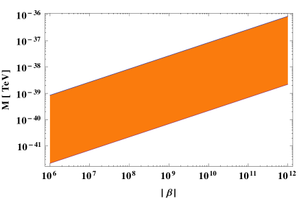
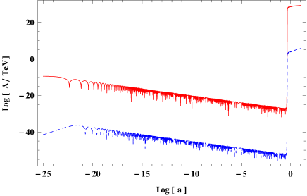
Figure 3: Left panel: Parameter space, for $|\beta|>10^{6}$ in which the symmetry is broken outside the galaxy and unbroken inside so that fifth force and Lorentz violations are screened. Right panel: Cosmological evolution of the temporal (dashed blue) and the spatial (solid red) components of the vector field, where we can see how the symmetry breaking takes place and the field goes to the new minimum and oscillates there.

Although the field hides in high density regions, at cosmological scales the symmetry can be broken and astrophysical signatures appear. In the early universe (radiation and matter dominated epochs), we expect the vector field to be subdominant. In such a case, it is justified to consider the equations for the vector field and assume that the expansion is driven by the dominant component. As before, we assume that the vector field is spacelike. This means that we have ${\mathcal{A}}_{i}\equiv A_{i}/a\gg A_{0}$. Moreover, we assume that the spatial component has linear polarisation along the $z$-direction. Then, in a FLRW metric, the equations of motion are given by

$$\ddot{A}_{0}+3H\dot{A}_{0} = \left[-3\dot{H}+M^{2}+2\frac{T\beta}{M_{pl}^{2}}e^{\beta(A_{0}^{2}-{\mathcal{A}}_{z}^{2})/M_{p}^{2}}\right]A_{0}$$ (19)

$$\ddot{{\mathcal{A}}}_{z}+3H\dot{{\mathcal{A}}}_{z} = \left[M^{2}-\dot{H}-2H^{2}+2\frac{T\beta}{M_{p}^{2}}e^{\beta(A_{0}^{2}-{\mathcal{A}}_{z}^{2})/M_{p}^{2}}\right]{\mathcal{A}}_{z}.$$

We have solved these equations numerically throughout the universe evolution and the solutions are plotted in Figure 3. In the following we shall find approximate analytical solutions for the cosmological evolution. Since the coupling to the background density is through the trace of the energy-momentum tensor, only non-relativistic species are relevant for the interactions of the vector field, i.e., only the matter component will modify the effective mass of the vector field. Thus, we can simply set $T=\rho_{m}$, even in the radiation dominated epoch. Moreover, we also assume that $A_{0}^{2},{\mathcal{A}}_{z}^{2}\ll M_{p}^{2}/\beta$ so that we can approximate the exponential by 1. Notice that, as long as this condition holds, the equations decouple and both components evolve independently. Well inside the radiation dominated epoch the equations can be approximated by

$$\ddot{A}_{0}+3H\dot{A}_{0} \simeq -3\dot{H}A_{0},$$ (20)

$$\ddot{{\mathcal{A}}}_{z}+3H\dot{{\mathcal{A}}}_{z} \simeq 0$$

where we have used that $T\simeq 0$ and $H^{2}\gg M^{2}$. Thus, the growing mode for the temporal component is given by $A_{0}\propto t$, whereas ${\mathcal{A}}_{z}$ remains frozen. This behaviour goes on until the energy density of matter becomes relevant in the field equations. This will imply that we need to tune the initial conditions such that, even though $A_{0}$ grows with respect to ${\mathcal{A}}_{z}$, it remains smaller ($A_{0}<{\mathcal{A}}_{z}$) by the time when $\rho_{m}$ starts being relevant. If we look at the equations, we can see that this happens when $2\beta\rho_{m}/M_{p}^{2}\simeq H^{2}\simeq\rho_{r}/M_{p}^{2}$, i.e., when $\rho_{r}\simeq 2\beta\rho_{m}$. The corresponding redshift is $(1+z_{T})=2\beta\Omega_{m}/\Omega_{r}=2\beta(1+z_{\rm eq})$ with $z_{\rm eq}$ the equality redshift. Thus, provided that $\beta>1$, this indeed happens in the radiation dominated epoch. After this time, the matter component becomes relevant and the equations can be approximated by:

$$\ddot{A}_{0}+3H\dot{A}_{0} = \frac{2\beta\rho_{m}}{M_{pl}^{2}}A_{0},$$ (21)

$$\ddot{{\mathcal{A}}}_{z}+3H\dot{{\mathcal{A}}}_{z} = \frac{(2\beta-\frac{1}{6})\rho_{m}}{M_{pl}^{2}}{\mathcal{A}}_{z},$$ (22)

where we have used that $\dot{H}+2H^{2}=\frac{1}{6M_{p}^{2}}T$. Since we are assuming a negative value for $\beta$, the solutions are damped oscillations for both components. During radiation, the damping factor is $t^{-1/4}$, whereas in the matter epoch it is $t^{-1/2}$ for both components. The field behaves in this way until $M^{2}\sim\beta H^{2}$. At this point, the effective mass becomes negative and the field grows exponentially until ${\mathcal{A}}^{2}\sim|M_{p}^{2}/\beta|$, when the higher order terms become important. This happens because the critical density at which the symmetry breaking occurs is reached and the field evolves towards the new minimum. Once the new minimum is reached, the field starts oscillating around it. However, since the position of the minimum is time-dependent, with a timescale of order $\beta\rho/M_{p}^{2}$, the center of the oscillations moves. This is so because the oscillations timescale is

$$\tau^{-2}\sim m_{\rm eff}^{2}\sim M^{2}\log\frac{-M^{2}M_{p}^{2}}{2\beta\rho}\sim M^{2}\log\frac{-M^{2}}{2\beta H}$$

and the timescale associated with the evolution of the minimum is $H^{-1}$, so that we have that $\frac{m_{\rm eff}^{2}}{H^{2}}\sim\frac{M^{2}}{H^{2}}\log\frac{-M^{2}}{2\beta H^{2}}$, that is large after the symmetry breaking. Therefore, the minimum evolves adiabatically with respect to the field oscillations.

Notice that during Big Bang nucleosynthesis the field is cosmologically screened so that no effects are present and the corresponding constraints are easily evaded.

The main difference between these models and GR comes from an anisotropic effective gravitational constant which will affect structure formation at large scales. Moreover, these models will have imprints in cosmology which are not present in other screening models, such as the chameleons and symmetron type of models. Those signatures will arise from the novel extra-term in the energy-momentum tensor (4) proportional to $A_{\mu}A_{\nu}$ that can produce anisotropic stresses on large scales that will contribute to the ISW effect.

In summary, a screening mechanism for conformal vector-tensor modifications of general relativity is proposed. Such mechanism allows to screen a vector field on small scales while non-trivial cosmological effects can still be present due to modifications of Einstein’s equations. We focus on a simple model consisting of a massive vector field which is conformally coupled to matter. The screening mechanism occurs due to a spontaneous symmetry breaking, therefore is applicable to a whole class of theories with different combinations of potential and conformal couplings so that the vector field is either timelike or spacelike at the critical points after the symmetry breaking. Moreover, our mechanisms also provides a way to restore Lorentz invariance in high dense regions, while being broken in low dense regions. This is a novel and unique signature of this mechanism. Notice also that in spite of local gravity constraints being easily evaded, the cosmological structure formation within these theories will be different from both General Relativity and other screened-modified gravities, due to the coupling between matter and the vector field. Finally the screening mechanism operating on small scales opens a new avenue for fundamental vector fields strongly coupled to matter into our theories.

Appendix

In this Appendix we intend to briefly comment on the relation of our action with the Stueckelberg action for a massive vector field. To show that, we consider the theory in flat spacetime and that the vector field is much smaller than the Planck mass. In such a limit, the conformal relation can be approximated by

$$\tilde{g}_{\mu\nu}\simeq\left(1+\frac{2\beta A^{2}}{M_{p}^{2}}\right)\eta_{\mu\nu},$$ (23)

with $\eta_{\mu\nu}$ the Minkowski metric. Then, we can plug this expression into the action to obtain the following action for the vector field

$$S=\int d^{4}x\left[-\frac{1}{4}F^{2}-\frac{1}{2}(\partial_{\mu}A^{\mu})^{2}+\frac{1}{2}M_{\rm eff}A^{2}]\right].$$ (24)

where we have defined

$$M_{\rm eff}^{2}\equiv-\frac{M^{2}}{2}\left(1+\frac{2\beta}{M_{p}^{2}}\tilde{g}^{\alpha\beta}\tilde{T}_{\alpha\beta}\right).$$ (25)

Notice that this is nothing but the mass $m_{0}^{2}$ obtained for the field in the phase without symmetry breaking. Now, we remind the action for a massive vector field in the Stueckelberg formalism (see for instance [18])

$$S=\frac{1}{2}\int d^{4}x\left[-\partial_{\mu}A_{\nu}\partial^{\mu}A^{\nu}+m^{2}A^{2}+\partial_{\mu}\varphi\partial^{\mu}\varphi-m^{2}\varphi^{2}\right]$$ (26)

where $\varphi$ is a scalar field (the Stueckelberg field). After integrating by parts, dropping surface terms and recasting the resulting terms, the Stueckelberg action can be written as

$$S=\int d^{4}x\left[-\frac{1}{4}F^{2}-\frac{1}{2}\left(\partial_{\mu}A^{\mu}+m\varphi\right)^{2}+\frac{m^{2}}{2}\left(A_{\mu}+\frac{1}{m}\partial_{\mu}\varphi\right)^{2}\right].$$ (27)

From this form of the action, it is more apparent that it exhibits a gauge symmetry $A_{\mu}\rightarrow A_{\mu}+\partial_{\mu}\Lambda$, $\varphi\rightarrow\varphi+m\Lambda$, with the gauge function satisfying the wave equation $(\Box+m^{2})\Lambda=0$. It is also apparent that our action reduces to Stueckelberg action in a gauge with $\varphi=0$, which can be chosen since the restriction of the gauge parameter coincides with the equation of $\varphi$. Another way of interpreting our action is as the Stueckelberg action in which we neglect $\varphi$ (not necessarily imposed by a gauge condition). We also remind here that to guarantee the consistency of the theory at the quantum level, it is necessary to impose the following additional subsidiary condition:

$$(\partial_{\mu}A^{\mu}+m\varphi)^{(-)}\big{|}{\mathrm{phys}}\big{\rangle}=0$$ (28)

where, the superscript ^(-) denotes the positive frequency part of the operator (i.e., it only involves annihilation operators) and $\big{|}{\mathrm{phys}}\big{\rangle}$ is the space of physical states. This is nothing but the analogous of the Gupta-Bleuler condition implemented for the massive case. Thus, one works in a space of indefinite metric, but the physical states have positive norm and the Hamiltonian is also positive definite on the physical space.

Instead of using our action without the Stueckelberg field, one could alternatively consider the full action including $\varphi$. In such a case, to maintain the gauge invariance, the conformal relation should also include the Stueckelberg field

$$\tilde{g}_{\mu\nu}=B^{2}(x)g_{\mu\nu},$$ (29)

where the argument of the conformal factor is $x\equiv(A_{\mu}+\frac{1}{m}\partial_{\mu}\varphi)^{2}$.

It is important to notice that going from the flat spacetime version of the action for a massive vector field to its curved spacetime version is not free from the usual ambiguity when covariantising a given action by replacing ordinary partial derivatives with covariant derivatives. One could covariantise either (26) or (27) and one would end up with different curved spacetime versions of the same theory in flat spacetime. The difference between both actions will be a non-minimal coupling of the vector field to the curvature, more precisely, a term $R_{\mu\nu}A^{\mu}A^{\nu}$. Although this term would give rise to a different cosmological evolution or different features in contexts where curvature is relevant, it is important to note that, since it vanishes in a Minkowski spacetime, it does not affect the screening mechanism proposed in this Letter, which would equally work for both versions of the covariant action.

References

References

- [1] T. Clifton, P. G. Ferreira, A. Padilla and C. Skordis, Phys. Rept. 513 (2012) 1 [arXiv:1106.2476 [astro-ph.CO]].
- [2] T. P. Sotiriou and V. Faraoni, Rev. Mod. Phys. 82 (2010) 451 [arXiv:0805.1726 [gr-qc]].
- [3] A. De Felice and S. Tsujikawa, Living Rev. Rel. 13 (2010) 3 [arXiv:1002.4928 [gr-qc]].
- [4] J. Khoury and A. Weltman, Phys. Rev. Lett. 93 (2004) 171104 [astro-ph/0309300].
- [5] J. A. R. Cembranos, Phys. Rev. D 73 (2006) 064029 [gr-qc/0507039].
- [6] K. Hinterbichler and J. Khoury, Phys. Rev. Lett. 104 (2010) 231301 [arXiv:1001.4525 [hep-th]].
- [7] A. Vainshtein, Phys.Lett B39, 393 (1972)
- [8] T. S. Koivisto, D. F. Mota and M. Zumalacarregui, Phys. Rev. Lett. 109 (2012) 241102 [arXiv:1205.3167 [astro-ph.CO]].
- [9] A. E. Nelson and J. Walsh, Phys. Rev. D 77 (2008) 095006 [arXiv:0802.0762 [hep-ph]].
- [10] J. A. Zuntz, P. G. Ferreira and T. G. Zlosnik, Phys. Rev. Lett. 101 (2008) 261102 [arXiv:0808.1824 [gr-qc]].
- [11] B. Li, D. Fonseca Mota and J. D. Barrow, Phys. Rev. D 77 (2008) 024032 [arXiv:0709.4581 [astro-ph]].
- [12] D. Bekenstein, Phys. Rev. D 70 (2004) 083509
- [13] H. Gies, D. F. Mota and D. J. Shaw, Phys. Rev. D 77 (2008) 025016 [arXiv:0710.1556 [hep-ph]].
- [14] S. M. Carroll and E. A. Lim, Phys. Rev. D 70 (2004) 123525 [hep-th/0407149].
- [15] L. Ford, Phys. Rev. D40, 967 (1989). A. Golovnev, V. Mukhanov and V. Vanchurin, JCAP 0806 (2008) 009 [arXiv:0802.2068 [astro-ph]].
- [16] C. G. Boehmer and T. Harko, Eur. Phys. J. C 50 (2007) 423 [gr-qc/0701029]. J. Beltran Jimenez and A. L. Maroto, Phys. Rev. D 78 (2008) 063005 [arXiv:0801.1486 [astro-ph]]. J. Beltran Jimenez and A. L. Maroto, JCAP 0903 (2009) 016 [arXiv:0811.0566 [astro-ph]]. J. Beltran Jimenez and A. L. Maroto, Phys. Lett. B 686 (2010) 175 [arXiv:0903.4672 [astro-ph.CO]]. J. Beltran Jimenez, T. S. Koivisto, A. L. Maroto and D. F. Mota, JCAP 0910 (2009) 029 [arXiv:0907.3648 [physics.gen-ph]]. T. Koivisto and D. F. Mota, JCAP 0808 (2008) 021 [arXiv:0805.4229 [astro-ph]].
- [17] K. Dimopoulos, Phys. Rev. D 74 (2006) 083502 [hep-ph/0607229]. K. Dimopoulos and M. Karciauskas, JHEP 0807 (2008) 119 [arXiv:0803.3041 [hep-th]]. K. Dimopoulos, M. Karciauskas and J. M. Wagstaff, Phys. Rev. D 81 (2010) 023522 [arXiv:0907.1838 [hep-ph]]. M. Karciauskas and D. H. Lyth, JCAP 1011 (2010) 023 [arXiv:1007.1426 [astro-ph.CO]].
- [18] H. Ruegg and M. Ruiz-Altaba, Int. J. Mod. Phys. A 19 (2004) 3265 [hep-th/0304245].
- [19] T. Jacobson and D. Mattingly, Phys. Rev. D 64 (2001) 024028 [gr-qc/0007031]. T. Jacobson, PoS QG -PH (2007) 020 [arXiv:0801.1547 [gr-qc]].
- [20] G. Esposito-Farese, C. Pitrou and J. -P. Uzan, Phys. Rev. D 81 (2010) 063519 [arXiv:0912.0481 [gr-qc]].
- [21] J. A. R. Cembranos, C. Hallabrin, A. L. Maroto and S. J. N. Jareno, Phys. Rev. D 86 (2012) 021301 [arXiv:1203.6221 [astro-ph.CO]]. J. A. R. Cembranos, A. L. Maroto and S. J. N. Jareno, Phys. Rev. D 87 (2013) 043523 [arXiv:1212.3201 [astro-ph.CO]].
- [22] P. Brax, Phys. Lett. B 712 (2012) 155 [arXiv:1202.0740 [hep-ph]].