Flow past superhydrophobic surfaces with cosine variation in local slip length

Abstract

Anisotropic super-hydrophobic surfaces have the potential to greatly reduce drag and enhance mixing phenomena in microfluidic devices. Recent work has focused mostly on cases of super-hydrophobic stripes. Here, we analyze a relevant situation of cosine variation of the local slip length. We derive approximate formulae for maximal (longitudinal) and minimal (transverse) directional effective slip lengths that are in good agreement with the exact numerical solution and lattice-Bolzmann simulations for any surface slip fraction. The cosine texture can provide a very large effective (forward) slip, but it was found to be less efficient in generating a transverse flow as compared to super-hydrophobic stripes.

I Introduction

The design and fabrication of textured superhydrophobic surfaces have received much attention in recent years. If the recessed regions of the texture are filled with gas (the Cassie state), roughness can produce remarkable liquid mobility, dramatically lowering the ability of drops to stick quere.d:2008 . These surfaces are known to be self-cleaning and show low adhesive forces. In addition to the self-cleaning effect, they also exhibit drag reduction for fluid flow. Thus, they are of importantance in the context of transport phenomena and fluid dynamics as well bocquet2007 ; vinogradova.oi:2011 ; rothstein.jp:2010 . Many sea animals e.g. shark and other fish are known to possess superhydrophobic skin bhushan.b:2011 . Also many artificial textures have been designed to increase drag reduction efficiency vinogradova.oi:2012 .

This drag reduction is associated with the liquid slippage past solid surfaces. This slippage occurs at smooth hydrophobic surfaces and can be described by the boundary condition vinogradova.oi:1999 ; bocquet2007 ; lauga2005 , $u_{\rm slip}=b\,\partial u/\partial z$, where $u_{\rm slip}$ is the (tangential) slip velocity at the wall, $\partial u/\partial z$ the local shear rate, and $b$ the slip length. A mechanism for hydrophobic slippage involves a lubricating gas layer of thickness $\delta$ with viscosity $\mu_{g}$ much smaller than that of the liquid $\mu$ vinogradova.oi:1995a , so that $b\simeq\delta(\mu/\mu_{g}-1)\simeq 50\delta$ vinogradova.oi:1995a ; andrienko.d:2003 . However, at smooth flat hydrophobic surfaces $\delta$ is small, so that $b$ cannot exceed a few tens of nm vinogradova.oi:2003 ; vinogradova.oi:2009 ; charlaix.e:2005 ; joly.l:2006 . In case of superhydrophobic surfaces, the situation can change dramatically, and slip lengths up to tens of $\mu$m may be obtained over a thick gas layer stabilized with a rough texture choi.ch:2006 ; joseph.p:2006 .

To quantify the flow past heterogeneous surfaces it is convenient to apply the concept of an effective slip boundary condition at the imaginary smooth homogeneous, but generally anisotropic surface vinogradova.oi:2011 ; Kamrin_etal:2010 . Such an effective condition mimics the actual one along the true heterogeneous surface, and fully characterizes the real flow. The quantitative understanding of the effective slip length of the superhydrophobic surface, $\mathbf{b}_{\mathrm{eff}}$, is still challenging since the composite nature of the texture in addition to liquid-gas areas requires regions of lower local slip (or no slip) in direct contact with the liquid. For an anisotropic texture, the effective slip generally depends on the direction of the flow and is a tensor, $\mathbf{b}_{\mathrm{eff}}\equiv\{b_{ij}^{\mathrm{eff}}\}$ represented by a symmetric, positive definite $2\times 2$ matrix Bazant08

$$\mathbf{b}_{\mathrm{eff}}=\mathbf{S}_{\theta}\left(\begin{array}[]{cc}b_{\mathrm{eff}}^{\parallel}&0\\ 0&b_{\mathrm{eff}}^{\perp}\end{array}\right)\mathbf{S}_{-\theta},$$ (1)

diagonalized by a rotation

$$\mathbf{S}_{\theta}=\left(\begin{array}[]{cc}\cos\theta&\sin\theta\\ -\sin\theta&\cos\theta\end{array}\right).$$

Eq.(1) allows us to calculate an effective slip in any direction given by an angle $\theta$, provided the two eigenvalues of the slip-length tensor, $b_{\mathrm{eff}}^{\parallel}$ ($\theta=0$) and $b_{\mathrm{eff}}^{\perp}$ ($\theta=\pi/2$), are known. The concept of an effective slip length tensor is general and can be applied for an arbitrary channel thickness harting.j:2012 , being a global characteristic of a channel vinogradova.oi:2011 , so that the eigenvalues normally depend not only on the parameters of the heterogeneous surfaces, but also on the channel thickness. However, for a thick (compared to a texture period, $L$) channel we are interested in here they become a characteristics of a heterogeneous interface solely.

In case of an anisotropic isolated surface (or a thick channel limit) with a scalar local slip $b(y)$, varying in only one direction, the transverse component of the slip-length tensor was proven to be equal to a half of the longitudinal one with twice larger local slip, $2b(y)$ asmolov:2012

$$b_{\mathrm{eff}}^{\bot}\left[b\left(y\right)/L\right]=\frac{b_{\mathrm{eff}}^{\parallel}\left[2b\left(y\right)/L\right].}{2}$$ (2)

A remarkable corollary of this relation is that the flow along any direction of the one-dimensional surface can be easily determined, once the longitudinal component of the effective slip tensor is found from the known spatially nonuniform scalar slip.

One-dimensional superhydrophobic surfaces are very important for a class of phenomena, which involves “transverse” hydrodynamic couplings, where an applied pressure gradient or shear rate in one direction generates flow in a different direction, with a nonzero perpendicular component. This can be used to mix adjacent streams, control the dispersion of plugs, and position streams within the cross section of the channel stroock2002b . Such grooved surfaces can be easily prepared by modern lithographic methods vinogradova.oi:2012 .

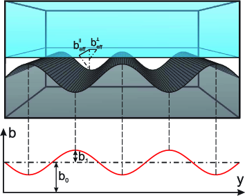
Figure 1: (Color online) Sketch of the SH surface with a cosine relief, and its equivalent representation in terms of flow boundary conditions.

Most of the prior work focussed on a flat, periodic, striped superhydrophobic surface, which corresponds to patterns of rectangular grooves. The flow past such stripes was tackled theoretically  lauga.e:2003 ; belyaev.av:2010a ; feuillebois.f:2009 ; vinogradova.oi:2011 ; feuillebois.f:2010b ; ng:2009 , and several numerical approaches have also been used either at the molecular scale, using molecular dynamics priezjev.n:2011 , or at larger mesoscopic scales using finite element methods priezjev.nv:2005 ; cottin.c:2004 , lattice Boltzmann harting.j:2012 and dissipative particle dynamics zhou.j:2012 simulations. For a pattern composed of no-slip ($b=0$) and perfect-slip ($b=\infty$) stripes, the expression for the eigenvalues of the effective slip-length tensor takes its maximum possible value and reads philip.jr:1972 ; lauga.e:2003

$$b_{\mathrm{ideal}}^{\parallel}=2b_{\mathrm{ideal}}^{\perp}=-\frac{L}{\pi}\ln\left[\sec\left(\frac{\pi\left(1-\phi\right)}{2}\right)\right],$$ (3)

where $\phi$ is the fraction of the no-slip interface. In the limit of vanishing solid fraction, it therefore predicts $b_{\mathrm{ideal}}^{\parallel}$ and $b_{\mathrm{ideal}}^{\perp}$ to depend only logarithmically on $\phi$ and scale as $-L\ln\phi$. At a qualitative level, this result means that the effective slip lengths essentially saturate at the value fixed by the period of the roughness. In case of stripes the perturbation of piecewise constant local slip has a step-like jump on the heterogeneity boundary, which leads to a singularity both in pressure and velocity gradient asmolov:2012 by introducing an additional mechanism for a dissipation. It is natural to assume that an anisotropic one-dimensional texture with a continuous local slip could potentially lead to a larger effective tensorial slip.

In this paper we address the issue of the effective slip of flat surfaces with cosine variation in the local slip length, which corresponds to modulated hydrophobic grooved surfaces with a trapped gas layer (the Cassie state) as shown in Fig. 1. Flows over hydrophilic surfaces (the Wenzel state) with cosine surface relief of small amplitude have been studied by a number of authors stroock2002b ; hocking.lm:1976 ; wang2004 ; priezjev.nv:2006 ; niavarani.a:2010 . Previous studies of similar grooves in the Cassie state have investigated only small variations in local slip length hocking.lm:1976 ; hendy2005effect . We are unaware of any previous work that has studied the most interesting case of finite and large variations in the amplitude of a local cosine slip.

II Theory

Consider a shear flow over a textured flat slipping plate, characterized by a slip length $b(y)$, spatially varying in one direction, and the texture varying over a period $L$ (as shown in Fig. 1). We use a rectangular coordinate system $(x,y,z)$ with origin at the wall. The $z-$ axis is perpendicular to the plate. Our analysis is based on the limit of a thick channel or a single interface, so that the velocity profile sufficiently far above the surface, at a height large compared to $L$, may be considered as a linear shear flow. All variables are non-dimensionalized using the texture period $L$ as the characteristic length, the shear rate of the undisturbed flow $G$ and the fluid viscosity $\mu.$

The dimensionless fluid velocity is sought in the form

$$\mathbf{v}=\mathbf{U}+\mathbf{u}_{\rm slip}+\mathbf{u}_{1}\left(x,y,z\right),$$

where $\mathbf{U}=z\mathbf{e}_{l},\ l=x,y$ is the undisturbed linear shear flow, and $\mathbf{e}_{l}\$are the unit vectors parallel to the plate. The perturbation of the flow, which is caused by the presence of the texture, involves a constant slip velocity $\mathbf{u}_{\rm slip}=\left(u_{\rm slip},v_{\rm slip},0\right)$ and a varying part $\mathbf{u}_{1}=\left(u,v,w\right)$ of the velocity field. A periodic velocity $\mathbf{u}_{1}$ should decay at infinity and has zero average:

$$\int_{0}^{1}\mathbf{u}_{1}dy=0.$$ (4)

At a small Reynolds number $Re=GL^{2}/\nu,$ $\mathbf{u}_{1}$ satisfies the dimensionless Stokes equations,

$$\mathbf{\nabla}\cdot\mathbf{u}_{1}=0,$$ (5)

$$\mathbf{\nabla}p-\Delta\mathbf{u}_{1}=\mathbf{0}.$$

The boundary conditions at the wall and at infinity are defined in the usual way as

$$z=0:\quad\mathbf{u}_{\rm slip}+\mathbf{u}_{1\tau}-\beta\left(y\right)\frac{\partial\mathbf{u}_{1\tau}}{\partial z}=\beta\left(y\right)\mathbf{e}_{l},\$$ (6)

$$w=0,$$ (7)

$$z\rightarrow\infty:\quad\mathbf{u}_{1}=\mathbf{0,}$$ (8)

where $\mathbf{u}_{1\tau}=\left(u,v,0\right)$ is the velocity along the wall and $\beta=b/L$ is the normalized local slip length. The eigenvalues of the effective slip-length tensor can be obtained as the components of $\mathbf{u}_{\rm slip}:$

$$b_{\mathrm{eff}}^{\parallel}=Lu_{\rm slip},\quad b_{\mathrm{eff}}^{\perp}=Lv_{\rm slip}.$$ (9)

III Cosine slip length

In this Section we consider a 1D periodic texture with the local slip length

$$\beta=\beta_{0}+2\beta_{1}\cos\left(2\pi y\right).$$ (10)

The coefficients should satisfy $\beta_{0}\geq 2\beta_{1}\geq 0,~{}$in order to obey $\beta\left(y\right)\geq 0$ for any $y.$

The disturbance velocity field is presented in terms of Fourier series as

$$\mathbf{u}_{1}=\sum_{n=-\infty,n\neq 0}^{\infty}\mathbf{u}^{\ast}\left(n,z\right)\exp\left(i2\pi ny\right),\quad\mathbf{u}^{\ast}=\left(u^{\ast},v^{\ast},w^{\ast}\right).$$ (11)

A general solution of the Stokes equations for the longitudinal flow, $\mathbf{U}=z\mathbf{e}_{x}$ decaying at infinity, reads asmolov:2012

$$u^{\ast}=X_{n}\exp\left(-2\pi\left|n\right|z\right),$$ (12)

$$v^{\ast}=w^{\ast}=0,$$

and that for the transverse flow, $\mathbf{U}=z\mathbf{e}_{y}$ is given by

$$u^{\ast}=0,$$

$$v^{\ast}=Y_{n}\exp\left(-2\pi\left|n\right|z\right)\left(1-2\pi nz\right),$$ (13)

$$w^{\ast}=-i2\pi nY_{n}z\exp\left(-2\pi\left|n\right|z\right).$$ (14)

The Fourier coefficients $X_{n}$ and $Y_{n}$ are determined from the Navier slip boundary condition (6).

III.1 Longitudinal configuration

Since the local slip length is an even function of $y,$ the solution (11) is also an even function. This requires $X_{n}=X_{-n},$ so it is sufficient to evaluate $X_{n}$ for $n\geq 0.$ The Navier slip boundary condition (6) can be written, following to asmolov:2012 , in terms of Fourier coefficients as a linear system

$$u_{\rm slip}=\beta_{0}-2e_{1}X_{1},$$ (15)

$$d_{1}X_{1}+e_{2}X_{2}=\beta_{1},$$ (16)

$$n>1:\quad e_{n-1}X_{n-1}+d_{n}X_{n}+e_{n+1}X_{n+1}=0,$$ (17)

$$d_{n}=1+2\pi n\beta_{0},\quad e_{n}=2\pi n\beta_{1}.$$ (18)

A three-diagonal infinite linear system (15)-(17) should be solved numerically to find teh unknown $X_{n}$ by truncating the system.

In the limit of large slip, $\beta_{0}>2\beta_{1}\gg 1,$ the asymptotic solution to (15)-(17) can also be constructed. To the leading order in $\beta_{0}^{-1}$, the first term in (18) can be neglected compared to the second one, and the system (16)-(17) is rewritten for new variables $t_{n}=2\pi nX_{n}$ as

$$t_{1}+\lambda t_{2}=\lambda,$$ (19)

$$n>1:\quad\lambda t_{n-1}+t_{n}+\lambda t_{n+1}=0,$$ (20)

where $\lambda=\beta_{1}/\beta_{0}<1/2.$ The solution of the last system is a geometric progression, $t_{n+1}=q^{n}t_{1},$ with

$$q=\frac{-\lambda^{-1}+\sqrt{\lambda^{-2}-4}}{2},$$

$$t_{1}=\frac{\lambda}{1+q\lambda}=\frac{\beta_{1}}{\beta_{0}+q\beta_{1}}.$$

Therefore, the final expression for the slip length, $b_{\mathrm{eff}}^{\parallel}=Lu_{\rm slip}$, in view of (15), takes the following form at $\beta_{0}>2\beta_{1}\gg 1:$

$$b_{\mathrm{eff}}^{\parallel}=\sqrt{b_{0}^{2}-4b_{1}^{2}}.$$ (21)

The asymptotic solution for the velocity field can also be derived from Eqs.(11) and (12). The normal component of velocity gradient can be written as

$$\frac{\partial u}{\partial z}=-2t_{1}\sum_{n=1}^{\infty}q^{n-1}\mathrm{Re}\left\{\exp\left[2\pi n\left(iy-z\right)\right]\right\}.$$ (22)

The factor $2$ is due to the contribution of $n<0.$ The sum in (22) is also a geometric progression, so that

$$\frac{\partial u}{\partial z}=-\frac{2t_{1}\exp\left(-2\pi z\right)\left[\cos\left(2\pi y\right)-q\exp\left(-2\pi z\right)\right]}{s},$$ (23)

$$s=1-2q\cos\left(2\pi y\right)\exp\left(-2\pi z\right)+q^{2}\exp\left(-4\pi z\right).$$

The last equation can be integrated over $z$ to give

$$u=-\frac{t_{1}}{2\pi q}\ln s.$$ (24)

The asymptotic solutions (21), (23) and (24) predict well the numerical data even at finite $b_{0}$ (see next Section).

III.2 Transverse configuration

It was found by asmolov:2012 that the velocity components for the transverse flow can be expressed in terms of the longitudinal one calculated for twice larger local slip, $u_{2}=u\left[2\beta\left(y\right)\right]:$

$$v_{\rm slip}=\frac{u_{slip,2}}{2},$$ (25)

$$v = \frac{1}{2}\left(u_{2}+z\frac{\partial u_{2}}{\partial z}\right),$$ (26)

$$w = -\frac{z}{2}\frac{\partial u_{2}}{\partial y}.$$ (27)

Using (9) and (25) we derive

$$b_{\mathrm{eff}}^{\perp}=b_{\mathrm{eff}}^{\parallel}=\sqrt{b_{0}^{2}-4b_{1}^{2}}.$$ (28)

Thus, the texture is isotropic at large $b_{0}$. One can demonstrate that the conclusion about isotropy of the slip-length tensor is general and valid for any textures (see Appendix A).

The values $\lambda,q,t_{1}$ remain the same for the double slip length since they depend on the ratio $\beta_{1}/\beta_{0}$ only. As a result, we obtain

$$u_{2}=u=-\frac{t_{1}}{2\pi}\ln s,$$

$$v = -\frac{t_{1}}{4\pi q}\ln s$$

$$- \frac{zt_{1}\exp\left(-2\pi z\right)\left[\cos\left(2\pi y\right)-q\exp\left(-2\pi z\right)\right]}{s},$$

$$w = \frac{zt_{1}\exp\left(-2\pi z\right)\sin\left(2\pi y\right)}{s}.$$ (30)

IV Simulation method

For the modelling of fluid flow in a system of two parallel plates, we employ the lattice Boltzmann (LB) method  bib:succi-01 . Lattice Boltzmann methods are derived by a phase space discretization of the kinetic Boltzmann equation

$$\left[\frac{\partial}{\partial t}+\mathbf{v}\cdot\nabla_{\mathbf{r}}\right]f(\mathbf{r,v},t)=\mathbf{\Omega},$$ (31)

which expresses the dynamics of the single particle probability density $f(\mathbf{r},\mathbf{v},t)$. Therein, $\mathbf{r}$ is the position, $\mathbf{v}$ the velocity, and $t$ the time. The left-hand side models the propagation of particles in phase space, the collision operator $\mathbf{\Omega}$ on the right hand side accounts for particle interactions.

Constructing the lattice Boltzmann equation, the time $t$, the position $\mathbf{r}$, and the velocity $\mathbf{v}$ are discretized. This discrete variant of Eq. (31)

$$\begin{array}[]{cc}f_{k}(\mathbf{r}+\mathbf{c}_{k},t+1)-f_{k}(\mathbf{r},t)=\Omega_{k},&k=0,1,\dots,B,\end{array}$$ (32)

describes the kinetics in discrete time- ($\Delta t$) and space-units ($\Delta x$). We employ a widely used three-dimensional lattice with $B=18$ discrete non-zero velocities (D3Q19) which is chosen to carry sufficient symmetry to allow for a second order accurate solution of the Navier-Stokes equations. Here, for $\Omega$, we choose the Bhatnagar-Gross-Krook (BGK) collision operator bib:bgk

$$\Omega_{k}=-\frac{1}{\tau}\left(f_{k}(\mathbf{r},t)-f_{k}^{eq}(\mathbf{v}(\mathbf{r},t),\rho(\mathbf{r},t))\right)\mbox{ ,}$$ (33)

which assumes relaxation on a linear timescale $\tau$ towards a discretized local Maxwell-Boltzmann distribution $f_{k}^{eq}$. The kinematic viscosity $\nu=\frac{2\tau-1}{6}$ of the fluid is related to the relaxation time scale. In this study it is kept constant at $\tau=1.0$.

Stochastic moments of $f$ can be related to physical properties of the modelled fluid. Here, conserved quantities, like the fluid density $\rho(\mathbf{r},t)=\rho_{0}\sum_{k}f_{k}(\mathbf{r},t)$ and momentum $\rho(\mathbf{r},t)\mathbf{u}(\mathbf{r},t)=\rho_{0}\sum_{k}c_{k}f_{k}(\mathbf{r},t)$, with $\rho_{0}$ being a reference density, are of special interest.

Slip over hydrophobic surfaces is commonly modelled by introduction of a phenomenological repulsive force  bib:jens-kunert-herrmann:2005 ; bib:jens-jari:2008 ; bib:zhu-tretheway-petzold-meinhart-2005 ; bib:benzi-etal-06 ; bib:zhang-kwok-04 . The magnitude of interactions between different components and surfaces, as determined by simulation parameters allows to specify arbitrary contact-angles  benzi-etal-06b ; bib:huang-thorne-schaap-sukop-2007 ; bib:jens-schmieschek:2010 ; bib:jens-kunert-herrmann:2005 . Other approaches include boundary conditions taking into account specular reflections succi02 ; bib:tang-tao-he-2005 ; bib:sbragaglia-succi-2005 , or diffuse scattering bib:ansumaili-karlin-2002 ; bib:sofonea-sekerka-2005 ; bib:niu-shu-chew-2004 , respectively. The strategy applied for this work employs a second order accurate on-site fixed velocity boundary condition to simulate wall slippage. Here, the velocity at the boundary is set proportional to the local stress imposed by the flow field as well as a slip length parameter adjusting the stress-response. For the details of the implementation we refer the reader to HechtHarting2010 ; ahmed.nk:2009 . Local slip lengths are calculated according to Eq. (10). Varying slip patterns are applied to the $x$-$y$-plane at $z=0$. Periodic boundary conditions are employed in $x$ and $y$-direction, thus reducing the simulation domain to a pseudo-2D system. By exploiting the periodic boundaries, only one single period needs to be resolved. The Couette flow is driven by applying a constant velocity of $v=0.1$ (in lattice units) in the $x$-$y$-plane at $z=z_{\rm max}$.

The resolution of the simulated system is given by the lattice constant

$$\Delta x=\frac{H}{\mathcal{N}},$$ (34)

where $\mathcal{N}$ is the number of discretization points used to resolve the height of the channel. As we consider thick channels, we choose a height to periodicity ratio of $H/L=10$.

The number of timesteps required to reach a steady state depends on the channel height, the velocity of the flow as determined by the driving acceleration as well as the fraction of slip and no slip area at the surface. We find that in order to reduce the deviation from theoretical predicted values below 5 percent, a domain size of $96\times 1\times 960\Delta x^{3}$ is required. For this geometrical setup, with a shear rate in the order of $\dot{\gamma}=1\cdot 10^{-4}$ (in lattice units), a simulation time in the order of 10 million timesteps is needed to reach the steady state. We compare the theoretical predictions by measurements of $b_{\mathrm{eff}}$ obtained from velocity profiles. The profile of the linear shear velocity is fit by a linear function in the region far from the surface pattern. From this fit the effective slip lengths and shear rate are determined.

V Results and discussion

In this section, we present the LB simulation results and compare them with predictions of the continuous theory.

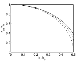
Figure 2: Eigenvalues of the effective slip-length tensor as a function of $b_{1}$ simulated at fixed $b_{0}=1$ (symbols). The longitudinal effective slip length, $b_{\mathrm{eff}}^{\parallel}$, is shown by circles, and the transverse effective slip, $b_{\mathrm{eff}}^{\perp}$ is presented by diamonds. Solid and dashed curves denote the corresponding theoretical values obtained by numerical Fourier-series solutions. The asymptotic (isotropic) solution, Eq. (28), expected in the limit $b_{0}\gg L$ is shown by the dash-dotted line.

We start with varying the amplitude of cosine perturbations of the slip length, $b_{1}$, at fixed $b_{0}=1$. Fig. 2 shows simulation data for $b_{\mathrm{eff}}^{\parallel}\$ and $b_{\mathrm{eff}}^{\perp}$ as a function of $b_{1}/b_{0}$. These results show that the largest possible value of $b_{\mathrm{eff}}/b_{0}$ is attained when $b_{1}=0$, i.e. for a smooth hydrophobic surface with $b(y)=b_{0}$. In this situation the effective slip is (obviously) isotropic and equal to the area-averaged slip $b_{0}$. When increasing the amplitude $b_{1}$, there is a small anisotropy of the flow, and the eigenvalues of the slip-length tensor decrease. Therefore, in the presence of a cosine variation in slip length the effective slip always becomes smaller than average. This conclusion is consistent with earlier observations made for different textures alexeyev:96 ; vinogradova.oi:2011 . To obtain theoretical values, the linear system, Eqs. (15)-(17) has been solved numerically by using the IMSL-DLSLTR routine. We see that the agreement is excellent for all $b_{1}/b_{0}$, indicating that our asymptotic theory is extremely accurate, and confirming the relation (25) between the longitudinal and transverse slip lengths. Also included in Fig. 2 is the asymptotic formula (28) obtained in the limit of large $b_{0}$. Note that this formula is surprisingly accurate even in the case of finite $b_{0},$ except for the texture with $b_{1}/b_{0}=1/2$ (no-slip point at $y=1/2$).

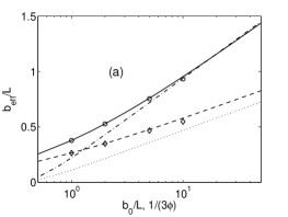
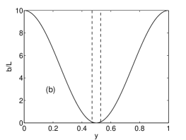
Figure 3: $\left(a\right)$ Effective slip lengths computed for $b_{1}/b_{0}=0.5$, which correspond to a texture with no-slip lines, vs. average slip. The notations are the same as in Fig. 2. Dash-dotted and dotted lines show the effective lengths for longitudinal and transverse stripes as a function of $1/(3\phi)$ calculated with Eq.(3). $\left(b\right)$ The cosine profile of the local slip length with $b_{0}/L=5,\ b_{1}/b_{0}=0.5$ (solid curve) and the stripe profile with $\phi=0.06$ (dashed line) with the same longitudinal effective slip lengths.

Fig. 3 $\left(a\right)$ shows the simulation data for effective slip lengths as a function of average slip, $b_{0}/L$, for a texture with the no-slip point $\left(b_{1}/b_{0}=1/2\right)$. Also included are theoretical (Fourier series) curves. The fits are quite good for $b_{0}/L$ up to 10, but at larger average slip there is some discrepancy. The simulation results for $b_{\mathrm{eff}}^{\parallel}$ and $b_{\mathrm{eff}}^{\perp}$ give smaller values than predicted by the theory. A possible explanation for this discrepancy is that the major contribution to the shear stress at large $b_{0}/L$ and $b_{1}/b_{0}=1/2$ comes from a very small region near the no-slip point (as we discuss below). The discretization error of the LB simulation becomes maximal in this region, and is particularly pronounced for the velocity gradients of systems with large effective slip. While we observe deviations around the no slip extremal value, the curves converge fast when stepping away from it and the excellent agreement of the measured effective slip suggest that the influenece of discretization errors on the mean flow is negligible at the resolution used. The asymptotic formula, Eq.(28), predicts $b_{\mathrm{eff}}=0$. This likely indicates that in this situation it is necessary to construct the second-order term of expansions for eigenvalues. At relatively large $b_{0}/L$, the effective slip lengths can be well fitted as

$$b_{\mathrm{eff}}^{\parallel}/L \simeq 0.1871+0.3175\ln\left(b_{0}/L+1.166\right),$$ (35)

$$b_{\mathrm{eff}}^{\perp}/L \simeq 0.2036+0.158\,8\ln\left(b_{0}/L+0.583\right).$$

In other words, they scale as $\ln(b_{0}/L)$ at large $b_{0}/L.$

Since the effective slip lengths for a texture decorated with perfect-slip stripes, Eq.(3), also shows a logarithmic growth (with $\phi$), in order to compare these two one-dimensional anisotropic textures the theoretical curve for stripes is included in Fig. 3$\left(a\right)$. It can be seen that in the limit of large average slip the asymptotic curves for longitudinal effective slip for stripes and cosine texture nearly coincide. This means that both textures generate the same forward flow in the longitudinal direction. Simple estimates suggest $b_{\mathrm{eff}}^{\parallel}\left(\beta_{0}\right)\simeq b_{\mathrm{ideal}}^{\parallel}\left[1/\left(3\beta_{0}\right)\right].$ Perhaps the most interesting and important aspect of this observation is that, from the point of view of the longitudinal effective slip, the “wide” cosine texture with $\beta_{0}=5$ taken for our numerical example is equivalent to the patterns of stripes with the extremely low fraction of no-slip regions, $\phi=0.06$ (see Fig. 3$\left(b\right)$). These results may guide the design of superhydrophobic surfaces for large forward flows in microfluidic devices. Note, however, that in the situation when longitudinal slip for both textures are similar, the cosine texture shows a larger transverse effective slip as seen in Fig. 3$\left(a\right)$. This means that textures with the cosine variation in the local slip length are less anisotropic than stripes, and $b_{\mathrm{eff}}^{\parallel}/b_{\mathrm{eff}}^{\perp}<b_{\mathrm{ideal}}^{\parallel}/b_{\mathrm{ideal}}^{\perp}=2$. Therefore, cosine textures are less optimal for a generation of robust transverse flows as compared with a sharp-edge stripe geometry.

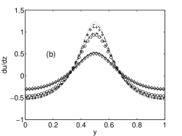
Figure 4: $\left(a\right)$ The velocities and $\left(b\right)\$the normal velocity gradients along the wall for the textures with $b_{1}/b_{0}=1/3,\ b_{0}/L=0.2$ (solid curve, diamonds)$,\ b_{0}/L=1$ (dashed curve, circles)$,\ b_{0}/L=5$ (dash-dotted line, crosses). Dotted curves show predictions of asymptotic formulae, Eqs. (24) and (23).

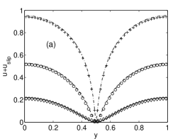
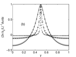
Figure 5: $\left(a\right)$ The velocities and $\left(b\right)\$the normal velocity gradients along the wall for the no-slip textures ($b_{1}/b_{0}=1/2$). Other notations are the same as in Fig. 4

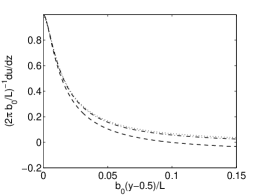
Figure 6: The normal velocity gradients for the no-slip textures with large amplitudes of slip length variation, $b_{0}/L=1$ (dashed curve)$,\ b_{0}/L=5$ (dash-dotted curve),$\ b_{0}/L=20$ (dotted curve) as functions of stretched coordinates.

The flow direction is associated with hydrodynamic pressures in the film, which is related to the heterogeneous slippage at the wall. Fig. 4 shows the profiles of the velocity and of the normal velocity gradient along the wall for different $\beta_{0}$ and $\beta_{1}/\beta_{0}>1/2$. The velocity dependence $u\left(x,y,0\right)$ is smooth, and $\frac{\partial u}{\partial z}\left(x,y,0\right)$ is finite for any $\beta_{0}$ and $\beta_{1}$, unlike the striped textures with piecewise-constant $\beta$ asmolov:2012 . Asymptotic predictions (24) and (23) are in a good agreement with numerical results and simulation data.

Similar theoretical and simulation results, but obtained for a texture with no-slip point, $\beta_{1}/\beta_{0}=1/2$, are shown in Fig. 5. In this situation we find that $\partial u/\partial z\left(1/2\right)=2\pi\beta_{0}$ for all $\beta_{0}$.

Finally, we should like to stress that a very small region near the no-slip point gives a main contribution to the shear stress at large $b_{0}/L.$ For the major portion of the texture far from this region, we have $\partial u/\partial z\simeq-1,$ so that the total shear stress is zero, and this part of the texture is shear-free. Since the maximum values of the normal velocity gradients grow like $b_{0}/L$ one can expect that a length scale of this small region is $L^{2}/b_{0}\ll L,$ or, equivalently, the curvature radius, $r=\left(d^{2}b/dy^{2}\right)^{-1}=L^{2}/\left(4\pi^{2}b_{0}\right)\ll L,$ at the no-slip point. The validity of this assumption is justified in Fig. 6, where the gradients for several values of $b_{0}/L$ versus stretched coordinates, $b_{0}\left(y-0.5\right)/L,$ are presented. The curves are very close for $b_{0}/L\geq 5$. Therefore, the normal gradient distribution and the dimensionless effective slip length in this case are controlled by the ratio $r/L$ only. These conclusions can be extended to any $b\left(y\right)$ characterized by a small radius $r=\left(d^{2}b/dy^{2}\right)^{-1}\ll L$ near the no-slip point and by a large slope, of the order of $L/r\gg 1$ or larger, far from it.

VI Conclusion

We have investigated shear flow past a super-hydrophobic surface with a cosine variation of the local slip length, and have evaluated resulting effective slippage and the flow velocity. We have found that the cosine texture can provide a very large effective (forward) slip, but generates a smaller transverse velocity to the main (forward) flow than discrete stripes considered earlier. Our approximate formulae for longitudinal and transversal directional effective slip lengths are validated by means of lattice Boltzmann simulations. Excellent quantitative agreement is found for the effective slippage as well as for the flow field. Slight deviations of the observed velocity gradient close to the no-slip extremal value can be explained by discretization errors.

Appendix A Effective slip for a flow past strongly slipping anisotropic patterns

In this Appendix we give some simple arguments showing that the flow becomes isotropic in case of large local slip, $\beta_{\min}=\min\left[\beta\left(y\right)\right]\gg 1.$ In this situation for arbitrary local slip length $\beta\left(y\right)$ the leading-order $\mathbf{b}_{\mathrm{eff}}$ can be obtained directly from the local slip boundary condition, Eq.(6), without a need to solve the Stokes equations. Indeed, if $\beta\gg 1$, Eq. (6) requires that the velocity at the surface is large,

$$\left|\mathbf{u}_{\rm slip}+\mathbf{u}_{1\tau}\left(x,y,0\right)\right|\sim\beta_{\min}\gg 1,$$

but the normal gradient is finite, $\left|\partial\mathbf{u}_{1\tau}\left(x,y,0\right)/\partial z\right|\sim 1.$ This can be fulfilled if only $\left|\mathbf{u}_{\rm slip}\right|\sim\beta_{\min}\gg 1,\quad\left|\mathbf{u}_{1\tau}\right|\sim 1.$ One can then divide Eq. (6) by $\beta$ to obtain

$$z=0:\quad\frac{\mathbf{u}_{\rm slip}}{\beta\left(y\right)}-\frac{\partial\mathbf{u}_{1\tau}}{\partial z}-\mathbf{e}_{l}=O\left(\beta_{\min}^{-1}\right).$$

Finally, by averaging of the last equation over the texture periods, and by using Eqs.(4) and Eq.(9) we can easily derive an expression for a leading-order effective slip:

$$b_{\mathrm{eff}}^{\perp}\simeq b_{\mathrm{eff}}^{\parallel}\simeq L\left[\int_{0}^{1}\frac{dy}{\beta\left(y\right)}\right]^{-1}.$$ (36)

It can be verified that our result, Eq.(28), is consistent with (36). Note that the expression

$$b_{\mathrm{eff}}^{\parallel}\simeq b_{\mathrm{eff}}^{\bot}\simeq\left(\frac{\phi}{b_{0}}+\frac{1-\phi}{b_{1}}\right)^{-1},$$ (37)

which has been obtained for stripes with $b_{0},b_{1}\gg L$ cottin.c:2004 and is similar to the addition rule for resistors in parallel, also satisfies Eq.(36).

References

- (1) D. Quere, Annu. Rev. Mater. Res., 2008, 38, 71–99.
- (2) L. Bocquet and J. L. Barrat, Soft Matter, 2007, 3, 685–693.
- (3) O. I. Vinogradova and A. V. Belyaev, J. Phys.: Condens. Matter, 2011, 23, 184104.
- (4) J. P. Rothstein, Annu. Rev. Fluid Mech., 2010, 42, 89–109.
- (5) B. Bhushan, Beilstein J. Nanotechnol., 2011, 2, 66–84.
- (6) O. I. Vinogradova and A. L. Dubov, Mendeleev Commun., 2012, 22, 229–236.
- (7) O. I. Vinogradova, Int. J. Miner. Proc., 1999, 56, 31–60.
- (8) E. Lauga, M. P. Brenner and H. A. Stone, in Handbook of Experimental Fluid Dynamics, ed. C. Tropea, A. Yarin and J. F. Foss, Springer, NY, 2007, ch. 19, pp. 1219–1240.
- (9) O. I. Vinogradova, Langmuir, 1995, 11, 2213.
- (10) D. Andrienko, B. Dünweg and O. I. Vinogradova, J. Chem. Phys., 2003, 119, 13106.
- (11) O. I. Vinogradova and G. E. Yakubov, Langmuir, 2003, 19, 1227–1234.
- (12) O. I. Vinogradova, K. Koynov, A. Best and F. Feuillebois, Phys. Rev. Lett., 2009, 102, 118302.
- (13) C. Cottin-Bizonne, B. Cross, A. Steinberger and E. Charlaix, Phys. Rev. Lett., 2005, 94, 056102.
- (14) L. Joly, C. Ybert and L. Bocquet, Phys. Rev. Lett., 2006, 96, 046101.
- (15) C. H. Choi, U. Ulmanella, J. Kim, C. M. Ho and C. J. Kim, Phys. Fluids, 2006, 18, 087105.
- (16) P. Joseph, C. Cottin-Bizonne, J. M. Benoǐ, C. Ybert, C. Journet, P. Tabeling and L. Bocquet, Phys. Rev. Lett., 2006, 97, 156104.
- (17) K. Kamrin, M. Z. Bazant and H. A. Stone, J. Fluid Mech., 2010, 658, 409–437.
- (18) M. Z. Bazant and O. I. Vinogradova, J. Fluid Mech., 2008, 613, 125–134.
- (19) S. Schmieschek, A. V. Belyaev, J. Harting and O. I. Vinogradova, Phys. Rev. E, 2012, 85, 016324.
- (20) E. S. Asmolov and O. I. Vinogradova, J. Fluid Mech., 2012, 706, 108–117.
- (21) A. D. Stroock, S. K. Dertinger, G. M. Whitesides and A. Ajdari, Anal. Chem., 2002, 74, 5306–5312.
- (22) E. Lauga and H. A. Stone, J. Fluid Mech., 2003, 489, 55–77.
- (23) A. V. Belyaev and O. I. Vinogradova, J. Fluid Mech., 2010, 652, 489–499.
- (24) F. Feuillebois, M. Z. Bazant and O. I. Vinogradova, Phys. Rev. Lett., 2009, 102, 026001.
- (25) F. Feuillebois, M. Z. Bazant and O. I. Vinogradova, Phys. Rev. E, 2010, 82, 055301(R).
- (26) C. Ng and C. Wang, Phys. Fluids, 2009, 21, 013602.
- (27) N. V. Priezjev, J. Chem. Phys., 2011, 135, 204704.
- (28) N. V. Priezjev, A. A. Darhuber and S. M. Troian, Phys. Rev. E, 2005, 71, 041608.
- (29) C. Cottin-Bizonne, C. Barentin, E. Charlaix, L. Bocquet and J. L. Barrat, Eur. Phys. J. E, 2004, 15, 427.
- (30) J. J. Zhou, A. V. Belyaev, F. Schmid and O. I. Vinogradova, J. Chem. Phys., 2012, 136, 194706.
- (31) J. R. Philip, J. Appl. Math. Phys., 1972, 23, 353–372.
- (32) L. M. Hocking, J. Fluid Mech., 1976, 76, 801–817.
- (33) C. Wang, Physics of Fluids, 2004, 16, 2136.
- (34) N. V. Priezjev and S. M. Troian, J. Fluid Mech., 2006, 554, 25–46.
- (35) A. Niavarani and N. V. Priezjev, Phys. Rev. E, 2010, 81, 011606.
- (36) S. C. Hendy, M. Jasperse and J. Burnell, Physical Review E, 2005, 72, 016303.
- (37) S. Succi, The lattice Boltzmann equation for fluid dynamics and beyond, Oxford University Press, 2001.
- (38) P. L. Bhatnagar, E. P. Gross and M. Krook, Phys. Rev., 1954, 94, 511.
- (39) J. Harting, C. Kunert and H. Herrmann, Europhys. Lett., 2006, 328–334.
- (40) J. Hyväluoma and J. Harting, Phys. Rev. Lett., 2008, 100, 246001.
- (41) L. Zhu, D. Tretheway, L. Petzold and C. Meinhart, J. Comp. Phys., 2005, 202, 181.
- (42) R. Benzi, L. Biferale, M. Sbragaglia, S. Succi and F. Toschi, Europhys. Lett., 2006, 74, 651.
- (43) J. Zhang and D. Y. Kwok, Phys. Rev. E, 2004, 70, 056701.
- (44) R. Benzi, L. Biferale, M. Sbragaglia, S. Succi and F. Toschi, Phys. Rev. E, 2006, 74, 021509.
- (45) H. Huang, D. T. Thorne, M. G. Schaap and M. C. Sukop, Phys. Rev. E, 2007, 76, 066701.
- (46) S. Schmieschek and J. Harting, Comm. Comp. Phys., 2011, 9, 1165.
- (47) S. Succi, Phys. Rev. Lett., 2002, 89, 064502.
- (48) G. H. Tang, W. Q. Tao and Y. L. He, Phys. Fluids, 2005, 17, 058101.
- (49) M. Sbragaglia and S. Succi, Phys. Fluids, 2005, 17, 093602.
- (50) S. Ansumali and I. V. Karlin, Phys. Rev. E, 2002, 66, 026311.
- (51) V. Sofonea and R. F. Sekerka, Phys. Rev. E, 2005, 71, 066709.
- (52) X. D. Niu, C. Shu and Y. T. Chew, Europhys. Lett., 2004, 67, 600.
- (53) M. Hecht and J. Harting, Journal of Statistical Mechanics: Theory and Experiment, 2010, 2010, P01018.
- (54) N. K. Ahmed and M. Hecht, J. Stat. Mech. - Theory and Exp., 2009, P09017.
- (55) A. A. Alexeyev and O. I. Vinogradova, Colloids Surfaces A, 1996, 108, 173 – 179.