We study the quantized topological terms in a weak-coupling gauge theory with gauge group $G_{g}$ and a global symmetry $G_{s}$ in $d$ space-time dimensions. We show that the quantized topological terms are classified by a pair $(G,\nu_{d})$, where $G$ is an extension of $G_{s}$ by $G_{g}$ and $\nu_{d}$ an element in group cohomology ${\cal H}^{d}(G,\mathbb{R}/\mathbb{Z})$. When $d=3$ and/or when $G_{g}$ is finite, the weak-coupling gauge theories with quantized topological terms describe gapped symmetry enriched topological (SET) phases (ie gapped long-range entangled phases with symmetry). Thus, those SET phases are classified by ${\cal H}^{d}(G,\mathbb{R}/\mathbb{Z})$, where $G/G_{g}=G_{s}$. We also apply our theory to a simple case $G_{s}=G_{g}=Z_{2}$, which leads to 12 different SET phases in 2+1D, where quasiparticles have different patterns of fractional $G_{s}=Z_{2}$ quantum numbers and fractional statistics. If the weak-coupling gauge theories are gapless, then the different quantized topological terms may describe different gapless phases of the gauge theories with a symmetry $G_{s}$, which may lead to different fractionalizations of $G_{s}$ quantum numbers and different fractional statistics (if in 2+1D).

Quantized topological terms in weak-coupling gauge theories with a global symmetry
and their connection to symmetry enriched topological phases

I Introduction

For a long time, we thought that Landau symmetry breaking theoryLandau (1937); Ginzburg and Landau (1950); Landau and Lifschitz (1958) describes all phases and phase transitions. In 1989, through a theoretical study of high $T_{c}$ superconducting model, we realized that there exists a new kind of orders – topological order – which cannot be described by Landau symmetry breaking theory.Wen (1989); Wen and Niu (1990); Wen (1990) Recently, it was found that topological orders are related to long range entanglements.Levin and Wen (2006); Kitaev and Preskill (2006) In fact, we can regard topological order as pattern of long range entanglementsChen et al. (2010) defined through local unitary (LU) transformations.Levin and Wen (2005); Verstraete et al. (2005); Vidal (2007)

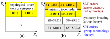
Figure 1: (Color online) (a) The possible gapped phases for a class of Hamiltonians $H(g_{1},g_{2})$ without any symmetry. (b) The possible gapped phases for the class of Hamiltonians $H_{\text{symm}}(g_{1},g_{2})$ with a symmetry. The yellow regions in (a) and (b) represent the phases with long range entanglement. Each phase is labeled by its entanglement properties and symmetry breaking properties. SRE stands for short range entanglement, LRE for long range entanglement, SB for symmetry breaking, SY for no symmetry breaking. SB-SRE phases are the Landau symmetry breaking phases. The SY-SRE phases are the SPT phases. The SY-LRE phases are the SET phases.

The notion of topological orders and long range entanglements leads to a more general and also more detailed picture of phases and phase transitions (see Fig. 1).Chen et al. (2010) For gapped quantum systems without any symmetry, their quantum phases can be divided into two classes: short range entangled (SRE) states and long range entangled (LRE) states.

SRE states are states that can be transformed into direct product states via LU transformations. All SRE states can be transformed into each other via LU transformations. So all SRE states belong to the same phase (see Fig. 1a), ie all SRE states can continuously deform into each other without closing energy gap and without phase transition.

LRE states are states that cannot be transformed into direct product states via LU transformations. It turns out that, in general, different LRE states cannot be connected to each other through LU transformations. The LRE states that are not connected via LU transformations represent different quantum phases. Those different quantum phases are nothing but the topologically ordered phases.

Chiral spin liquids,Kalmeyer and Laughlin (1987); Wen et al. (1989) fractional quantum Hall statesTsui et al. (1982); Laughlin (1983), $Z_{2}$ spin liquids,Read and Sachdev (1991); Wen (1991a); Moessner and Sondhi (2001) non-Abelian fractional quantum Hall states,Moore and Read (1991); Wen (1991b); Willett et al. (1987); Radu et al. (2008) etc are examples of topologically ordered phases. The mathematical foundation of topological orders is closely related to tensor category theoryFreedman et al. (2004); Levin and Wen (2005); Chen et al. (2010); Gu et al. (2010) and simple current algebra.Moore and Read (1991); Lu et al. (2010) Using this point of view, we have developed a systematic and quantitative theory for non-chiral topological orders in 2D interacting boson and fermion systems.Levin and Wen (2005); Chen et al. (2010); Gu et al. (2010) Also for chiral 2D topological orders with only Abelian statistics, we find that we can use integer $K$-matrices to describe them.Blok and Wen (1990); Read (1990); Fröhlich and Kerler (1991); Wen and Zee (1992); Belov and Moore (2005); Kapustin and Saulina (2011)

For gapped quantum systems with symmetry, the structure of phase diagram is even richer (see Fig. 1b). Even SRE states now can belong to different phases. One class of non-trivial SRE phases for Hamiltonians with symmetry is the Landau symmetry breaking states. But even SRE states that do not break the symmetry of the Hamiltonians can belong to different phases. The 1D Haldane phase for spin-1 chainHaldane (1983); Affleck et al. (1988); Gu and Wen (2009); Pollmann et al. (2009) and topological insulatorsKane and Mele (2005a); Bernevig and Zhang (2006); Kane and Mele (2005b); Moore and Balents (2007); Fu et al. (2007); Qi et al. (2008) are non-trivial examples of phases with short range entanglements that do not break any symmetry. We will call this kind of phases SPT phases. The term “SPT phase” may stand for Symmetry Protected Topological phase,Gu and Wen (2009); Pollmann et al. (2009) since the known examples of those phases, the Haldane phase and the topological insulators, were already referred as topological phases. The term “SPT phase” may also stand for Symmetry Protected Trivial phase, since those phases have no long range entanglements and have trivial topological orders.

It turns out that there is no gapped bosonic LRE state in 1D.Verstraete et al. (2005) So all 1D gapped bosonic states are either symmetry breaking states or SPT states. This realization led to a complete classification of all 1D gapped bosonic quantum phases.Chen et al. (2011a); Schuch et al. (2011); Chen et al. (2011b)

In LABEL:CLW1141,CGL1172, the classification of 1D SPT phase is generalized to any dimensions: For gapped bosonic systems in $d$ space-time dimensions with an on-site symmetry $G_{s}$, we can construct distinct SPT phases that do not break the symmetry $G_{s}$ from the distinct elements in ${\cal H}^{d}[G_{s},U(1)]$ – the $d$-cohomology class of the symmetry group $G_{s}$ with $U(1)$ as coefficient. We see that we have a quite systematic understanding of SRE states with symmetry.Levin and Stern (2009); Lu and Vishwanath (2012)

For gapped LRE states with symmetry, the possible quantum phases should be much richer than SRE states. We may call those phases Symmetry Enriched Topological (SET) phases. Projective symmetry group (PSG) was introduced to study the SET phases.Wen (2002, 2003); Wang and Vishwanath (2006) The PSG describes how the quantum numbers of the symmetry group $G_{s}$ get fractionalized on the gauge excitations.Wen (2003) When the gauge group $G_{g}$ is Abelian, the PSG description of the SET phases can be be expressed in terms of group cohomology: The different SET states with symmetry $G_{s}$ and gauge group $G_{g}$ can be (partially) described by ${\cal H}^{2}(G_{s},G_{g})$.Essin and Hermele (2012) Many examples of the SET states can be found in LABEL:W0213,KLW0834,KW0906,LS0903,YFQ1070.

Recently, Mesaros and Ran proposed a quite systematic understanding of a subclass of SET phases:Mesaros and Ran (2012) One can use the elements of ${\cal H}^{d}(G_{s}\times G_{g},\mathbb{R}/\mathbb{Z})$ to describe the SET phases in $d$ space-time dimensions with a finite gauge group $G_{g}$ and a finite global symmetry group $G_{s}$. Here ${\cal H}^{d}(G_{s}\times G_{g},\mathbb{R}/\mathbb{Z})$ is the group cohomology class of group $G_{s}\times G_{g}$. This result is based on the group cohomology theory of the SPT phasesChen et al. (2011d) and the Levin-Gu duality between the SPT phases and the “twisted” weak-coupling gauge theories.Levin and Gu (2012); Swingle (2012); Hung and Wen (2012) Also, Essin and Hermele generalized the results of LABEL:W0213,W0303a,KLW0834,KW0906 and studied quite systematically the SET phases described by a $G_{g}=Z_{2}$ gauge theory.Essin and Hermele (2012) They show that some of those SET phases can be classified by ${\cal H}^{2}(G_{s},G_{g})$.

In this paper, we will develop a somewhat systematic understanding of SET phases, following a path-integral approach developed for the group cohomology theory of the SPT phasesChen et al. (2011d) and the topological gauge theory.Dijkgraaf and Witten (1990); Hung and Wen (2012) The idea is to classify quantized topological terms in weak-coupling gauge theory with symmetry. If the weak-coupling gauge theory happens to have a gap, then the different quantized topological terms will describe different SET phases. This allows us to obtain and generalize the results in LABEL:MR1235,EH1293. Since weak-coupling gauge theories only describe some topological ordered states, our theory only describes some of the SET states.

We show that quantized topological terms in symmetric weak-coupling gauge theory in $d$ space-time dimensions with a gauge group $G_{g}$ and a global symmetry group $G_{s}$ can be described by a pair $(G,\nu_{d})$, where $G$ is an extension of $G_{s}$ by $G_{g}$ and $\nu_{d}$ is an element in ${\cal H}^{d}(G,\mathbb{R}/\mathbb{Z})$. (An extension of $G_{s}$ by $G_{g}$ is group $G$ that contain $G_{g}$ as a normal subgroup and satisfy $G/G_{g}=G_{s}$.) When $G_{g}$ is finite or when $d=3$, the weak-coupling gauge theory is gapped. In this case, $(G,\nu_{d})$ describe different SET phases. Note that the extension $G$ is nothing but the PSG introduced in LABEL:W0213. Also, when the symmetry group $G_{s}$ contains anti-unitary transformations, those anti-unitary transformations will act non-trivially on $\mathbb{R}/\mathbb{Z}$: $x\to-x$, $x\in\mathbb{R}/\mathbb{Z}$.Chen et al. (2011d)

In appendix B, we will show that we can use $(y_{0},y_{1},...,y_{d})$ with

$$y_{k}\in{\cal H}^{k}[G_{s},{\cal H}^{d-k}(G_{g},\mathbb{R}/\mathbb{Z})]$$ (1)

to label the elements in ${\cal H}^{d}(G,\mathbb{R}/\mathbb{Z})$. However, such a labeling may not be one-to-one and it may happen that only some of $(y_{0},y_{1},...,y_{d})$ correspond to the elements in ${\cal H}^{d}(G,\mathbb{R}/\mathbb{Z})$. But for every element in ${\cal H}^{d}(G,\mathbb{R}/\mathbb{Z})$, we can find a $(y_{0},y_{1},...,y_{d})$ that corresponds to it. If we choose a special extension $G=G_{g}\times G_{s}$, then we recover the result in LABEL:MR1235 if $G$ is finite: a set of SET states can be can be described by $(y_{0},y_{1},...,y_{d})$ with an one-to-one correspondence (see eqn. (A)):

$${\cal H}^{d}(G_{s}\times G_{g},\mathbb{R}/\mathbb{Z}) =\oplus_{p=0}^{d}{\cal H}^{d-p}[G_{s},{\cal H}^{p}(G_{g},\mathbb{R}/\mathbb{Z})]$$

$$=\oplus_{p=0}^{d}{\cal H}^{d-p}[G_{g},{\cal H}^{p}(G_{s},\mathbb{R}/\mathbb{Z})].$$ (2)

The term ${\cal H}^{d}[G_{s},{\cal H}^{0}(G_{g},\mathbb{R}/\mathbb{Z})]={\cal H}^{d}(G_{s},\mathbb{R}/\mathbb{Z})$ describes the quantized topological terms associated with only the symmetry $G_{s}$ which describe the SPT phases. The term ${\cal H}^{0}[G_{s},{\cal H}^{d}(G_{g},\mathbb{R}/\mathbb{Z})]={\cal H}^{d}(G_{g},\mathbb{R}/\mathbb{Z})$ describes the quantized topological terms associated with pure gauge theory. Other terms $\oplus_{p=1}^{d-1}{\cal H}^{d-p}[G_{s},{\cal H}^{p}(G_{g},\mathbb{R}/\mathbb{Z})]$ describe the quantized topological terms that involve both gauge theory $G_{g}$ and symmetry $G_{s}$. Those terms describe how $G_{s}$ quantum numbers get fractionalized on gauge-flux excitations.Mesaros and Ran (2012)

When $G_{g}$ is Abelian, the different extensions, $G$, of $G_{s}$ by $G_{g}$ is classified by ${\cal H}^{2}(G_{s},G_{g})$. This reproduces a result in LABEL:EH1293.

II A simple formal approach

First let us describe a simple formal approach that allows us to quickly obtain the above results. We know that the SPT phases in $d$-dimensional discrete space-time are described by topological non-linear $\sigma$-models with symmetry $G$:

$${\cal L}=\frac{1}{\lambda_{s}}[\partial g(x^{\mu})]^{2}+\hskip 1.0pt\mathrm{i}\hskip 1.0ptW_{\text{top}}(g),\ \ g\in G$$ (3)

where $\lambda_{s}\to\infty$, and the $2\pi$-quantized topological term $\int W_{\text{top}}(g)$ is given by an element in ${\cal H}^{d}(G,\mathbb{R}/\mathbb{Z})$. Different elements in ${\cal H}^{d}(G,\mathbb{R}/\mathbb{Z})$ describe different SPT phases.Chen et al. (2011d) If we “gauge” the symmetry $G$, the topological non-linear $\sigma$-model will become a gauge theory:

$${\cal L}=\frac{1}{\lambda_{s}}[(\partial-\hskip 1.0pt\mathrm{i}\hskip 1.0ptA)g(x^{\mu})]^{2}+\hskip 1.0pt\mathrm{i}\hskip 1.0ptW_{\text{top}}(g,A)+\frac{(F_{\mu\nu})^{2}}{\lambda},$$ (4)

where $W_{\text{top}}(g,A)$ is the gauged topological term. For those topological term that can be expressed in continuous field theory, $W_{\text{top}}(g,A)$ can be obtained from $W_{\text{top}}(g)$ by replacing $\partial_{\mu}$ by $\partial_{\mu}-\hskip 1.0pt\mathrm{i}\hskip 1.0ptA_{\mu}$. When $G_{s}$ and $G_{g}$ are finite, $W_{\text{top}}(g,A)$ can be constructed explicitly in discrete space-time.Zhang and Wen (2012)

If we further integrate out $g$, we will get a pure gauge theory with a topological term

$${\cal L}=\frac{(F_{\mu\nu})^{2}}{\lambda}+\hskip 1.0pt\mathrm{i}\hskip 1.0ptW_{\text{top}}(A).$$ (5)

This line of thinking suggests that the quantized topological term $\int\tilde{W}_{\text{top}}(A)$ in symmetric gauge theory is classified by the same ${\cal H}^{d}(G,\mathbb{R}/\mathbb{Z})$ that classifies the $2\pi$-quantized topological term $\int W_{\text{top}}(g)$.

Now let us consider topological non-linear $\sigma$-models with symmetry $G_{s}\times G_{g}$:

$${\cal L}=\frac{1}{\lambda_{s}}[\partial g(x^{\mu})]^{2}+\hskip 1.0pt\mathrm{i}\hskip 1.0ptW_{\text{top}}(g),\ \ g\in G=G_{s}\times G_{g},$$ (6)

where the $2\pi$-quantized topological term $\int W_{\text{top}}(g)$ is classified by ${\cal H}^{d}(G_{s}\times G_{g},\mathbb{R}/\mathbb{Z})$. If we “gauge” only a subgroup $G_{g}$ of the total symmetry group $G_{s}\times G_{g}$, we will get a gauge theory:

$${\cal L}=\frac{1}{\lambda_{s}}[(\partial-\hskip 1.0pt\mathrm{i}\hskip 1.0ptA)g(x^{\mu})]^{2}+\hskip 1.0pt\mathrm{i}\hskip 1.0ptW_{\text{top}}(g,A)+\frac{(F_{\mu\nu})^{2}}{\lambda}$$ (7)

with global symmetry $G_{s}$. This line of thinking suggests that the quantized topological term $\int W_{\text{top}}(g,A)$ is classified by the same ${\cal H}^{d}(G_{s}\times G_{g},\mathbb{R}/\mathbb{Z})$.

We can generalize the above approach to obtain more general quantized topological terms in weak-coupling gauge theory with gauge group $G_{g}$ and symmetry $G_{s}$. We start with a group $G$ which is an extension of the symmetry group $G_{s}$ by the gauge group $G_{g}$:

$$1\to G_{g}\to G\to G_{s}\to 1.$$ (8)

In other words, $G$ contains a normal subgroup $G_{g}$ such that $G/G_{g}=G_{s}$. So we can start with a topological non-linear $\sigma$-models with symmetry $G$:

$${\cal L}=\frac{1}{\lambda_{s}}[\partial g(x^{\mu})]^{2}+\hskip 1.0pt\mathrm{i}\hskip 1.0ptW_{\text{top}}(g),\ \ g\in G,$$ (9)

where the $2\pi$-quantized topological term $\int W_{\text{top}}(g)$ is classified by ${\cal H}^{d}(G,\mathbb{R}/\mathbb{Z})$. If we “gauge” only a subgroup $G_{g}$ of the total symmetry group $G$, we will get a gauge theory:

$${\cal L}=\frac{1}{\lambda_{s}}[(\partial-\hskip 1.0pt\mathrm{i}\hskip 1.0ptA)g(x^{\mu})]^{2}+\hskip 1.0pt\mathrm{i}\hskip 1.0ptW_{\text{top}}(g,A)+\frac{(F_{\mu\nu})^{2}}{\lambda}$$ (10)

with global symmetry $G_{s}=G/G_{g}$. This line of thinking suggests that the quantized topological term $\int W_{\text{top}}(g,A)$ is classified by ${\cal H}^{d}(G,\mathbb{R}/\mathbb{Z})$.

So more generally, the SET states in $d$-dimensional space-time with gauge group $G_{g}$ and symmetry group $G_{s}$ are labeled by the elements in ${\cal H}^{d}(G,\mathbb{R}/\mathbb{Z})$, where $G$ the extension of the symmetry group $G_{s}$ by the gauge group $G_{g}$, provided that the symmetric gauge theory (9) is gapped in small $\lambda$ limit and $d\geq 3$. If the symmetric gauge eqn. (9) is gapless in small $\lambda$ limit, then ${\cal H}^{d}(G,\mathbb{R}/\mathbb{Z})$ describes different gapless phases of the symmetric gauge theory.

The above approach is formal and hand-waving. When $G$ is finite, we can rigorously obtain the above results, which is described in LABEL:ZW. In the following, we will discuss such an approach assuming $G_{g}$ is finite (but $G_{s}$ can be finite or continuous). Then we will discuss another approach that allows us to obtain the above result more rigorously for the case $G=G_{s}\times G_{g}$ where $G_{s},G_{g}$ can be finite or continuous.

III An exact approach for finite $G_{g}$

This approach is based on the formal approach (10) discussed above, where $G$ is an extension of the symmetry group $G_{s}$ by the gauge group $G_{g}$: $G/G_{g}=G_{s}$. We will make the above approach exact by putting the theory on space-time lattice of $d$ dimensions.

III.0.1 Discretize space-time

We will discretize the space-time $M$ by considering its triangulation $M_{\text{tri}}$ and define the $d$-dimensional gauge theory on such a triangulation. We will call such a theory a lattice gauge theory. We will call the triangulation $M_{\text{tri}}$ a space-time complex, and a cell in the complex a simplex.

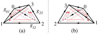
Figure 2: (Color online) Two branched simplices with opposite orientations. (a) A branched simplex with positive orientation and (b) a branched simplex with negative orientation.

In order to define a generic lattice theory on the space-time complex $M_{\text{tri}}$, it is important to give the vertices of each simplex a local order. A nice local scheme to order the vertices is given by a branching structure.Costantino (2005); Chen et al. (2011d) A branching structure is a choice of orientation of each edge in the $d$-dimensional complex so that there is no oriented loop on any triangle (see Fig. 2).

The branching structure induces a local order of the vertices on each simplex. The first vertex of a simplex is the vertex with no incoming edges, and the second vertex is the vertex with only one incoming edge, etc . So the simplex in Fig. 2a has the following vertex ordering: $0,1,2,3$.

The branching structure also gives the simplex (and its sub simplexes) an orientation denoted by $s_{ij...k}=1,*$. Fig. 2 illustrates two $3$-simplices with opposite orientations $s_{0123}=1$ and $s_{0123}=*$. The red arrows indicate the orientations of the $2$-simplices which are the subsimplices of the $3$-simplices. The black arrows on the edges indicate the orientations of the $1$-simplices.

III.0.2 Gauged non-linear $\sigma$-model on space-time lattice

To put (10) on space-time lattice, we put the $g(x^{\mu})\in G$ field on the vertices of the space-time complex, which becomes $g_{i}$ where $i$ labels the vertices. We also put the gauge field on the edges $ij$ which becomes $g_{ij}\in G_{g}$.

The action amplitude for a $d$-cell $(ij...k)$ is complex function of $g_{i}$ and $g_{ij}$: $V_{ij...k}(\{g_{ij}\},\{g_{i}\})$ The partition function is given by

$$Z=\sum_{\{g_{ij}\},\{g_{i}\}}\prod_{(ij...k)}[V_{ij...k}(\{g_{ij}\},\{g_{i}\})]^{s_{ij...k}}$$ (11)

where $\prod_{(ij...k)}$ is the product over all the $d$-cells $(ij...k)$. If the above action amplitude $\prod_{(ij...k)}[V_{ij...k}(\{g_{ij}\},\{g_{i}\})]^{s_{ij...k}}$ on closed space-time complex ($\partial M_{\text{tri}}=\emptyset$) is invariant under the gauge transformation

$$g_{ij}\to g^{\prime}_{ij}=h_{i}g_{ij}h_{j}^{-1},\ \ g_{i}\to g^{\prime}_{i}=h_{i}g_{i}h_{i}^{-1}\ \ \ h_{i}\in G_{g}$$ (12)

then the action amplitude $V_{ij...k}(\{g_{ij}\},\{g_{i}\})$ defines a gauge theory of gauge group $G_{g}$. If the action amplitude is invariant under the global transformation

$$g_{ij}\to g^{\prime}_{ij}=hg_{ij}h^{-1},\ \ g_{i}\to g^{\prime}_{i}=hg_{i}h^{-1}\ \ \ h\in G,$$ (13)

then the action amplitude $V_{ij...k}(\{g_{ij}\},\{g_{i}\})$ defines a gauge theory with a global symmetry $G_{s}=G/G_{g}$. (We need to mod out $G_{g}$ since when $h\in G_{g}$, it will generate a gauge transformation instead of a global symmetry transformation.)

Using a cocycle $\nu_{d}(g_{0},g_{1},...,g_{d})\in{\cal H}^{d}(G,\mathbb{R}/\mathbb{Z}),\ g_{i}\in G$, we can construct an action amplitude $V_{ij...k}(\{g_{ij}\},\{g_{i}\})$ that define a gauge theory with gauge group $G_{s}$ and global symmetry $G_{s}$. First, we note that the cocycle satisfies the cocycle condition

$$\nu_{d}(g_{0},g_{1},...,g_{d})=\nu_{d}(hg_{0},hg_{1},...,hg_{d}),\ \ \ h\in G$$

$$\prod_{i}\nu_{d}(g_{0},...,\hat{g}_{i},...,g_{d+1})=1$$ (14)

where $g_{0},...,\hat{g}_{i},...,g_{d+1}$ is the sequence $g_{0},...,g_{i},...,g_{d+1}$ with $g_{i}$ removed. The gauge theory action amplitude is given by

$$V_{01...d}(\{g_{ij}\},\{g_{i}\}) =0,\text{ if }g_{ij}g_{jk}\neq g_{ik}$$ (15)

$$V_{01...d}(\{g_{ij}\},\{g_{i}\}) =\nu_{d}(\tilde{g}_{0}g_{0},\tilde{g}_{1}g_{1},...,\tilde{g}_{d}g_{d}),\text{ otherwise},$$

where $\tilde{g}_{i}$ are given by

$$\tilde{g}_{0} =1, \tilde{g}_{1} =\tilde{g}_{0}g_{01}, \tilde{g}_{2} =\tilde{g}_{1}g_{12}, \tilde{g}_{3} =\tilde{g}_{2}g_{23},...$$ (16)

One can check that the above action amplitude $V_{01...d}(\{g_{ij}\},\{g_{i}\})$ is invariant under the gauge transformation (12) and the global symmetry transformation (13). Thus it defines an symmetric gauge theory

We know that the action amplitude is non-zero only when $g_{ij}g_{jk}=g_{ik}$. The condition $g_{ij}g_{jk}=g_{ik}$ is the flat connection condition, and the corresponding gauge theory is in the weak-coupling limit (actually is at the zero-coupling). This condition can be implemented precisely only when $G_{g}$ is finite. With the flat connection condition $g_{ij}g_{jk}=g_{ik}$, $\tilde{g}_{i}$’s and the gauge equivalent sets of $g_{ij}$ have an one-to-one correspondence.

Since the total action amplitude $\prod_{(ij...k)}[V_{ij...k}(\{g_{ij}\},\{g_{i}\})]^{s_{ij...k}}$ on a sphere is always equal to 1 if the gauge flux vanishes, therefore $V_{ij...k}(\{g_{ij}\},\{g_{i}\})$ describes a quantized topological term in weak-coupling gauge theory (or zero-coupling gauge theory). This way, we show that quantized topological term in a weak-coupling gauge theory with gauge group $G_{g}$ and symmetry group $G_{s}$ can be constructed from each element of ${\cal H}^{d}(G,\mathbb{R}/\mathbb{Z})$.

When $G_{g}=\{1\}$ (or $G=G_{s}$),

$$V_{01...d}(\{g_{ij}\},\{g_{i}\}) =\nu_{d}(g_{0},g_{1},...,g_{d})$$ (17)

become the action amplitude for the topological non-linear $\sigma$-model, describing the SPT phase labeled by the cocycle $\nu_{d}\in{\cal H}^{d}[G_{s},\mathbb{R}/\mathbb{Z})$.Chen et al. (2011d)

When $G_{s}=\{1\}$ (or $G=G_{g}$),

$$V_{01...d}(\{g_{ij}\},\{g_{i}\}) =\nu_{d}(\tilde{g}_{0}g_{0},\tilde{g}_{1}g_{1},...,\tilde{g}_{d}g_{d}).$$ (18)

We can use the gauge transformation (12) to set $g_{i}=1$ in the above and obtain

$$V_{01...d}(\{g_{ij}\},\{g_{i}\}) =\nu_{d}(\tilde{g}_{0},\tilde{g}_{1},...,\tilde{g}_{d}).$$ (19)

This is the topological gauge theory studied in LABEL:DW9093,HW1267.

IV An approach based on classifying space

In this section, we will consider the cases where $G_{s},G_{g}$ can be finite or continuous. But at time being, we can only handle the situation where $G=G_{s}\times G_{g}$. Our approach is based on the classifying space.

IV.1 Motivations and results

Let us first review some known results. To gain a systematic understand of SRE states with on-site symmetry $G_{s}$, we started with a non-linear $\sigma$-model

$${\cal L}=\frac{1}{\lambda_{s}}[\partial g(x^{\mu})]^{2},\ \ g\in G_{s}$$ (20)

with symmetry group $G_{s}$ as the target space. The model can be in a disordered phase that does not break the symmetry $G_{s}$ when $\lambda$ is large. By adding different $2\pi$ quantized topological $\theta$-terms to the Lagrangian ${\cal L}$, we can get different Lagrangians that describe different disordered phases that does not break the symmetry $G_{s}$.Chen et al. (2011d) Those disordered phases are the symmetry protected topological (SPT) phases.Gu and Wen (2009); Pollmann et al. (2009) So we can use the quantized topological terms to classify the SPT phases. (In general, topological terms, by definition, are the terms that do not depend on space-time metrics.)

We know that gauge theory

$${\cal L}=\frac{1}{\lambda}{\rm Tr}(F_{\mu\nu}F^{\mu\nu})$$ (21)

is one way to describe LRE states (ie topologically ordered states). In LABEL:DW9093,HW1267, different quantized topological terms in weak-coupling gauge theory with gauge group $G_{g}$ and small $\lambda$ in $d$ space-time dimensions are constructed and classified, using the topological cohomology class $H^{d+1}(BG_{g},\mathbb{Z})$ for the classifying space $BG_{g}$ of the gauge group $G_{g}$. By adding those quantized topological terms to the above Lagrangian for the weak-coupling gauge theory, we may obtain different phases of the weak-coupling gauge theory.

In this section, we plan to combine the above two approaches by studying the quantized topological terms in the combined theory

$${\cal L}=\frac{1}{\lambda}{\rm Tr}(F_{\mu\nu}F^{\mu\nu})+\frac{1}{\lambda_{s}}[\partial g(x^{\mu})]^{2},\ \ g\in G_{s}$$ (22)

where $F$ is the field strength with gauge group $G_{g}$, and $(\lambda,\lambda_{s})\to$ (small,large). Such a theory is a gauge theory with symmetry $G_{s}$. We find that quantized topological terms in the combined theory can be constructed and classified by the topological cohomology class $H^{d+1}(BG_{s}\times BG_{g},\mathbb{Z})$ for the classifying space of the product $G_{g}\times G_{s}$. Those quantized topological terms give us a somewhat systematic understanding of different phases of weak coupling gauge theories with symmetry. If those symmetric weak coupling gauge theories are gapped (for example, for finite gauge groups), then the theories will describe topologically ordered states with symmetry. Those SET phases in $d$ space-time dimensions are described by elements in $H^{d+1}(BG_{s}\times BG_{g},\mathbb{Z})$.

IV.2 Gauge theory as a non-linear $\sigma$-model with classifying space as the target space

To obtain the above result, we will follow closely the approaches used in LABEL:HW1267 and LABEL:CGL1172. We will obtained our result in two steps.

IV.2.1 Symmetric weak-coupling gauge theory as the non-linear $\sigma$-model of $G_{s}\times BG_{g}$

As in LABEL:HW1267, we may view a weak-coupling gauge theory with gauge group $G_{g}$ as a non-linear $\sigma$-model with classifying space $BG_{g}$ as the target space. So the symmetric weak-coupling gauge theory in eqn. (22) can be viewed as a non-linear $\sigma$-model with $G_{s}\times BG_{g}$ as the target space, where each path in the path integral is given by an embedding $\gamma:M_{\text{tri}}\to G_{s}\times BG_{g}$ from the space-time complex $M_{\text{tri}}$ to $G_{s}\times BG_{g}$. We can study topological terms in our symmetric weak-coupling gauge theory by studying the topological terms in the corresponding non-linear $\sigma$-model.

Following LABEL:HW1267, a total term $S_{\text{top}}$ corresponds to evaluating a cocycle $\alpha_{d}\in Z(G_{s}\times BG_{g},\mathbb{R}/\mathbb{Z})$ on the complex $\gamma(M_{\text{tri}})\subset G_{s}\times BG_{g}$:

$$S_{\text{top}}[\gamma]=2\pi\langle\alpha_{d},\gamma(M_{\text{tri}})\rangle\ \ \text{mod }2\pi.$$ (23)

Such a topological term does not depend on any smooth deformation of $\gamma$ and is thus “topological”. (Note that the evaluation of the $d$-cocycle on any $d$-cycles [ie $d$-dimensional closed complexes] are equal to $0$ mod 1 if the $d$-cycles are boundaries of some $(d+1)$-dimensional complex.)

Here we would like to stress that the cocycle $\alpha_{d}$ on the group manifold is not the ordinary topological cocycle. It has a symmetry condition

$$\langle\alpha_{d},c\rangle=\langle\alpha_{d},c_{g}\rangle$$ (24)

where $c$ is a complex in $G_{s}$, and $c_{g}$ is the complex generated from $c$ by the symmetry transformation $G_{s}\to gG_{s}$, $g\in G_{s}$. Also, since $\lambda_{s}\to\infty$ and $g(x^{\mu})$ have large fluctuations in eqn. (22), $\langle\alpha_{d},c\rangle$ only depend on the vertices $g_{0},g_{1},...$ of $c$:

$$\langle\alpha_{d},c\rangle =\nu(g_{0},g_{1},...),\ \ \ \ \nu(gg_{0},gg_{1},...)=\nu(g_{0},g_{1},...);$$

$$g,g_{i} \in G_{s}.$$ (25)

So, on $G_{s}$, $\alpha_{d}$ is actually a cocycle in the group cohomology ${\cal Z}(G_{s},\mathbb{R}/\mathbb{Z})$,Chen et al. (2011d) while on $BG_{g}$, $\alpha_{d}$ is the usual cocycle in the topological cohomology $Z(BG_{g},\mathbb{R}/\mathbb{Z})$.

Since, on $G_{s}$, $\alpha_{d}$ is a cocycle in the group cohomology ${\cal Z}(G_{s},\mathbb{R}/\mathbb{Z})$, when $G_{s}$ contain anti-unitary symmetry, such anti-unitary symmetry transformation will have a non-trivial action on $\mathbb{R}/\mathbb{Z}$: $x\to-x$, $x\in\mathbb{R}/\mathbb{Z}$.Chen et al. (2011d)

If two $d$-cocycles, $\alpha_{d},\alpha^{\prime}_{d}\in Z^{d}(BG_{g},\mathbb{R}/\mathbb{Z})$, differ by a coboundary: $\alpha^{\prime}_{d}-\alpha_{d}=\hskip 1.0pt\mathrm{d}\mu_{d}$, $\mu_{d}\in C^{d}(BG_{g},\mathbb{R}/\mathbb{Z})$, then, the corresponding action amplitudes, $\hskip 1.0pt\mathrm{e}^{\hskip 1.0pt\mathrm{i}\hskip 1.0ptS_{\text{top}}[\gamma]}$ and $\hskip 1.0pt\mathrm{e}^{\hskip 1.0pt\mathrm{i}\hskip 1.0ptS_{\text{top}}^{\prime}[\gamma]}$, can smoothly deform into each other without phase transition. So $\hskip 1.0pt\mathrm{e}^{\hskip 1.0pt\mathrm{i}\hskip 1.0ptS_{\text{top}}[\gamma]}$ and $\hskip 1.0pt\mathrm{e}^{\hskip 1.0pt\mathrm{i}\hskip 1.0ptS_{\text{top}}^{\prime}[\gamma]}$, or $\alpha_{d}$ and $\alpha^{\prime}_{d}$, describe the same quantum phase. Therefore, we regard $\alpha_{d}$ and $\alpha^{\prime}_{d}$ to be equivalent. The equivalent classes of the $d$-cocycles form the $d$ cohomology class $H^{d}(G_{s}\times BG_{g},\mathbb{R}/\mathbb{Z})$. We conclude that the topological terms in symmetric weak-coupling lattice gauge theories are described by $H^{d}(G_{s}\times BG_{g},\mathbb{R}/\mathbb{Z})$ in $d$ space-time dimensions.

To calculate $H^{d}(G_{s}\times BG_{g},\mathbb{R}/\mathbb{Z})$, let us first calculate $H^{d}(G_{s}\times BG_{g},\mathbb{Z})$. Using the the Künneth formula eqn. (A) (with $M^{\prime}=\mathbb{Z}$), we find that

$$\ \ \ \ H^{d}(G_{s}\times BG_{g},\mathbb{Z})$$

$$\simeq\Big{[}\oplus_{p=0}^{d}{\cal H}^{p}(G_{s},\mathbb{Z})\otimes_{\mathbb{Z}}H^{d-p}(BG_{g},\mathbb{Z})\Big{]}\oplus$$

$$\ \ \ \ \ \ \Big{[}\oplus_{p=0}^{d+1}\text{Tor}_{1}^{\mathbb{Z}}[{\cal H}^{p}(G_{s},{\mathbb{Z}}),H^{d-p+1}(BG_{g},\mathbb{Z})]\Big{]}.$$ (26)

In the above, we have used the fact that the cohomology on $G_{s}$ is the group cohomology ${\cal H}$ and the cohomology on $BG_{g}$ is the usual topological cohomology $H$.

In appendix A, we show that (see eqn. (73))

$$\ \ \ \ H^{d}(X,\mathbb{R}/\mathbb{Z})$$ (27)

$$\simeq H^{d}(X,\mathbb{Z})\otimes_{\mathbb{Z}}\mathbb{R}/\mathbb{Z}\oplus\text{Tor}_{1}^{\mathbb{Z}}[H^{d+1}(X,{\mathbb{Z}}),\mathbb{R}/\mathbb{Z}].$$

Using

$$\mathbb{Z}\otimes_{\mathbb{Z}}\mathbb{R}/\mathbb{Z}=\mathbb{R}/\mathbb{Z},\ \ \ \ \mathbb{Z}_{n}\otimes_{\mathbb{Z}}\mathbb{R}/\mathbb{Z}=0,$$

$$\text{Tor}_{1}^{\mathbb{Z}}(\mathbb{Z},\mathbb{R}/\mathbb{Z})=0,\ \ \ \ \text{Tor}_{1}^{\mathbb{Z}}(\mathbb{Z}_{n},\mathbb{R}/\mathbb{Z})=\mathbb{Z}_{n},$$ (28)

we see that $H^{d}(X,\mathbb{R}/\mathbb{Z})$ has a form $H^{d}(X,\mathbb{R}/\mathbb{Z})=\mathbb{R}/\mathbb{Z}\oplus...\oplus\mathbb{R}/\mathbb{Z}\oplus Z_{n_{1}}\oplus Z_{n_{2}}\oplus...$. So the discrete part of $H^{d}(X,\mathbb{R}/\mathbb{Z})$ is given by

$$\text{Dis}[H^{d}(X,\mathbb{R}/\mathbb{Z})] =Z_{n_{1}}\oplus Z_{n_{2}}\oplus...$$

$$=\text{Tor}[H^{d+1}(X,\mathbb{Z})],$$ (29)

where we have used

$$H^{d+1}(X,\mathbb{Z})=\text{Free}[H^{d+1}(X,\mathbb{Z})]\oplus\text{Tor}[H^{d+1}(X,\mathbb{Z})]$$ (30)

with $\text{Tor}[H^{d+1}(X,\mathbb{Z})]$ the torsion part and $\text{Free}[H^{d+1}(X,\mathbb{Z})]$ the free part of $H^{d+1}(X,\mathbb{Z})$. Therefore, we have

$$\ \ \ \ \text{Dis}[H^{d}(G_{s}\times BG_{g},\mathbb{R}/\mathbb{Z})]$$

$$\simeq\text{Tor}\Big{[}[\oplus_{p=0}^{d+1}{\cal H}^{p}(G_{s},\mathbb{Z})\otimes_{\mathbb{Z}}H^{d+1-p}(BG_{g},\mathbb{Z})]\oplus$$

$$\ \ \ \ \ \ [\oplus_{p=0}^{d+2}\text{Tor}_{1}^{\mathbb{Z}}({\cal H}^{p}(G_{s},{\mathbb{Z}}),H^{d-p+2}(BG_{g},\mathbb{Z}))]\Big{]}.$$ (31)

Since ${\cal H}^{d}(G_{s},\mathbb{Z})=H^{d}(BG_{s},\mathbb{Z})$, the above can be rewritten as

$$\ \ \ \ \text{Dis}[H^{d}(G_{s}\times BG_{g},\mathbb{R}/\mathbb{Z})]$$

$$\simeq\text{Tor}\Big{[}[\oplus_{p=0}^{d+1}H^{p}(BG_{s},\mathbb{Z})\otimes_{\mathbb{Z}}H^{d+1-p}(BG_{g},\mathbb{Z})]\oplus$$

$$\ \ \ \ \ \ [\oplus_{p=0}^{d+2}\text{Tor}_{1}^{\mathbb{Z}}(H^{p}(BG_{s},{\mathbb{Z}}),H^{d-p+2}(BG_{g},\mathbb{Z}))]\Big{]}$$

$$=\Big{[}\oplus_{p=0}^{d+1}\text{Tor}[H^{p}(BG_{s},\mathbb{Z})]\otimes_{\mathbb{Z}}\text{Tor}[H^{d+1-p}(BG_{g},\mathbb{Z})]\Big{]}\oplus$$

$$\ \ \ \ \Big{[}\oplus_{p=0}^{d+1}\text{Free}[H^{p}(BG_{s},\mathbb{Z})]\otimes_{\mathbb{Z}}\text{Tor}[H^{d+1-p}(BG_{g},\mathbb{Z})]\Big{]}\oplus$$

$$\ \ \ \ \Big{[}\oplus_{p=0}^{d+1}\text{Tor}[H^{p}(BG_{s},\mathbb{Z})]\otimes_{\mathbb{Z}}\text{Free}[H^{d+1-p}(BG_{g},\mathbb{Z})]\Big{]}\oplus$$

$$\ \ \ \ \Big{[}\oplus_{p=0}^{d+2}\text{Tor}_{1}^{\mathbb{Z}}(H^{p}(BG_{s},{\mathbb{Z}}),H^{d-p+2}(BG_{g},\mathbb{Z}))\Big{]}.$$ (32)

Each element in the above cohomology class describes a quantized topological term in the weakly coupled gauge theory with symmetry $G_{s}$.

IV.2.2 Chern-Simons form

We note that

$$\ \ \ \ H^{d+1}(BG_{s}\times BG_{g},\mathbb{Z})$$

$$=\Big{[}\oplus_{p=0}^{d+1}H^{p}(BG_{s},\mathbb{Z})\otimes_{\mathbb{Z}}H^{d+1-p}(BG_{g},\mathbb{Z})\Big{]}\oplus$$

$$\ \ \ \ \ \ \Big{[}\oplus_{p=0}^{d+2}\text{Tor}_{1}^{\mathbb{Z}}[H^{p}(BG_{s},{\mathbb{Z}}),H^{d-p+2}(BG_{g},\mathbb{Z})]\Big{]}.$$ (33)

So the result (IV.2.1) is very close to our proposal that elements in $H^{d+1}(BG_{s}\times BG_{g},\mathbb{Z})$ correspond to the quantized topological terms. The only thing missing is the free part of $H^{d}(BG_{g},\mathbb{Z})$.

In fact, the free part of $H^{d+1}(BG_{g},\mathbb{Z})$, denoted as Free$[H^{d+1}(BG_{g},\mathbb{Z})]$, is non-zero only when $d=$odd. So in the following, we will consider only $d$= odd cases. The free part Free$[H^{d+1}(BG_{g},\mathbb{Z})]$ corresponds to the Chern-Simons forms in $d$ space-time dimensions.

To understand such a result, we first choose a $\omega\in\text{Free}[H^{d+1}(BG_{g},\mathbb{Z})]$. We can find integers $K_{i}$ such that

$$-\omega+\frac{K_{1}}{\frac{d+1}{2}!(2\pi)^{\frac{d+1}{2}}}{\rm Tr}F^{\frac{d+1}{2}}+\cdots$$ (34)

is an exact form $\hskip 1.0pt\mathrm{d}\theta_{d}(A)$. Here $\theta_{d}(A)$ is called a Chern-Simons form in $d$-dimensions.

We can use a Chern-Simons form $\theta_{d-p}(A)$ and a cocycle $\alpha_{p}\in{\cal H}^{p}(G_{s},\mathbb{Z})$ to construct a quantized topological term

$$S_{\text{top}}[\gamma]=2\pi\langle\alpha_{p}\cup\theta_{d-p}(A),\gamma(M_{\text{tri}})\rangle\ \ \text{mod }2\pi.$$ (35)

Such kind of topological terms are labeled by the elements in

$$\ \ \ \ \oplus_{p=0}^{d+1}{\cal H}^{p}(G_{s},\mathbb{Z})\otimes_{\mathbb{Z}}\text{Free}[H^{d+1-p}(BG_{g},\mathbb{Z})]$$

$$=\oplus_{p=0}^{d+1}H^{p}(BG_{s},\mathbb{Z})\otimes_{\mathbb{Z}}\text{Free}[H^{d+1-p}(BG_{g},\mathbb{Z})].$$ (36)

Combining the above result with eqn. (IV.2.1), we find that the elements in $H^{d+1}(BG_{s}\times BG_{g},\mathbb{Z})$ correspond to the quantized topological terms.

V An example: $G_{s}=Z_{2}$ and $G_{g}=Z_{2}$

In this section, we will discuss a simple example with $G_{s}=Z_{2}$ and $G_{g}=Z_{2}$. There are two kinds of extensions $G$ of $G_{s}=Z_{2}$ by $G_{g}=Z_{2}$: $G=Z_{2}\times Z_{2}$ and $G=Z_{4}$. So the quantized topological terms and the SET phases are described by ${\cal H}^{d}(Z_{2}\times Z_{2},\mathbb{R}/\mathbb{Z})$ and ${\cal H}^{d}(Z_{4},\mathbb{R}/\mathbb{Z})$ in $d$ space-time dimensions.

In $d=3$ space-time dimensions, we have

$${\cal H}^{3}(Z_{2}\times Z_{2},\mathbb{R}/\mathbb{Z})=\mathbb{Z}_{2}^{3},\ \ \ {\cal H}^{3}(Z_{4},\mathbb{R}/\mathbb{Z})=\mathbb{Z}_{4}.$$ (37)

So there are 12 SET phases for weak-coupling $Z_{2}$ gauge theory with $Z_{2}$ symmetry. However, at this stage, it is not clear if those 12 SET phases are really distinct, since they could be smoothly connected via strong coupling gauge theory. Later, we will see that the 12 SET phases are indeed distinct, since they have distinct physical properties.

V.1 A $K$-matrix approach

To understand the physical properties of those 12 SET phases, we would like to use Levin-Gu duality to gauge the $G_{s}$ and turn the theory into gauge theory with gauge group $G$.

Let us first consider the $G=Z_{2}\times Z_{2}$ case. A $G=Z_{2}\times Z_{2}$ gauge theory can be described by $U^{4}(1)$ mutual Chern-Simons theory:Hansson et al. (2004); Kou et al. (2008)

$${\cal L}=\frac{1}{4\pi}K_{0,IJ}a^{I}_{\mu}\partial_{\nu}a^{J}_{\lambda}+...$$ (38)

with

$$K_{0}=2\begin{pmatrix}0&1&0&0\\ 1&0&0&0\\ 0&0&0&1\\ 0&0&1&0\\ \end{pmatrix}$$ (39)

The $G_{s}$ charge corresponds to the unit charge of $a^{1}_{\mu}$ gauge field and the $G_{g}$ gauge charge corresponds to the unit charge of $a^{3}_{\mu}$ gauge field. The $G_{s}$ flux excitation (in the $G=Z_{2}\times Z_{2}$ gauge theory) corresponds to the end of branch-cut in the original theory along which we have a twist generated by a $G_{s}$ symmetry transformation (see LABEL:LG1220 for a detailed discussion about the symmetry twist). Such $G_{s}$-flux correspond to the flux of $a^{1}_{\mu}$ gauge field.

The 8 types of quantized topological terms are given by

$$W_{\text{top}}=\frac{n_{1}}{2\pi}a^{1}_{\mu}\partial_{\nu}a^{1}_{\lambda}+\frac{n_{12}}{2\pi}a^{1}_{\mu}\partial_{\nu}a^{3}_{\lambda}+\frac{n_{2}}{2\pi}a^{3}_{\mu}\partial_{\nu}a^{3}_{\lambda}$$ (40)

$n_{1}=0,1$, $n_{12}=0,1$, $n_{2}=0,1$. The total Lagrangian has a form

$${\cal L}+W_{\text{top}}=\frac{1}{4\pi}K_{IJ}a^{I}_{\mu}\partial_{\nu}a^{J}_{\lambda}+...$$ (41)

with

$$K=\begin{pmatrix}2n_{1}&2&n_{12}&0\\ 2&0&0&0\\ n_{12}&0&2n_{2}&2\\ 0&0&2&0\\ \end{pmatrix}.$$ (42)

Two $K$-matrices are equivalent: $K_{1}\sim K_{2}$ if $K_{1}=U^{T}K_{2}U$ for an integer matrix with det$(U)=\pm 1$. We find $K(n_{1},n_{12},n_{2})\sim K(n_{1}+2,n_{12},n_{2})\sim K(n_{1},n_{12}+2,n_{2})\sim K(n_{1},n_{12},n_{2}+2)$. Thus only $n_{1},n_{12},n_{2}=0,1$ give rise to inequivalent $K$-matrices.

A particle carrying $l_{I}$ $a^{I}_{\mu}$-charge will have a statistics

$$\theta_{l}=\pi l_{I}(K^{-1})^{IJ}l_{J}.$$ (43)

A particle carrying $l_{I}$ $a^{I}_{\mu}$-charge will have a mutual statistics with a particle carrying $\tilde{l}_{I}$ $a^{I}_{\mu}$-charge:

$$\theta_{l,\tilde{l}}=2\pi l_{I}(K^{-1})^{IJ}\tilde{l}_{J}.$$ (44)

We note that the $G_{s}$ charge is identified with the unit $a^{1}_{\mu}$-charge and the $G_{g}$ gauge charge is identified with the unit $a^{3}_{\mu}$-charge. Using

$$K^{-1}=\frac{1}{4}\begin{pmatrix}0&2&0&0\\ 2&-2n_{1}&0&-n_{12}\\ 0&0&0&2\\ 0&-n_{12}&2&-2n_{2}\\ \end{pmatrix},$$ (45)

we find that the $G_{s}$ charge (the unit $a^{1}_{\mu}$-charge) and the $G_{g}$ gauge charge (the unit $a^{3}_{\mu}$-charge) remain bosonic after inclusion of the topological terms. This is actually a condition on the topological terms: the topological terms do not affect the statistics of the gauge charge.

$(n_{1}n_{12}n_{2})=(000)$
$(l_{1}l_{2}l_{3}l_{4})$	$G_{s}$-charge	$G_{s}$-twist	$G_{g}$-gauge	statistics
(0000)	0	0	0	0
(1000)	1	0	0	0
(0010)	0	0	e	0
(1010)	1	0	e	0
(0001)	0	0	m	0
(1001)	1	0	m	0
(0011)	0	0	em	1
(1011)	1	0	em	1
(0100)	0	1	0	0
(1100)	1	1	0	1
(0110)	0	1	e	0
(1110)	1	1	e	1
(0101)	0	1	m	0
(1101)	1	1	m	1
(0111)	0	1	em	1
(1111)	1	1	em	0

Table 1: The $G_{s}$-charges, the $G_{s}$-twists, the $G_{g}$-gauge sectors, and the statistics of the 16 kinds of quasiparticles/defects in the SET state $(n_{1}n_{12}n_{2})$.

$(n_{1}n_{12}n_{2})=(010)$
$(l_{1}l_{2}l_{3}l_{4})$	$G_{s}$-charge	$G_{s}$-twist	$G_{g}$-gauge	statistics
(0000)	0	0	0	0
(1000)	1	0	0	0
(0010)	0	0	e	0
(1010)	1	0	e	0
(0001)	$-1/2$	0	m	0
(1001)	$1/2$	0	m	0
(0011)	$-1/2$	0	em	1
(1011)	$1/2$	0	em	1
(0100)	0	1	0	0
(1100)	1	1	0	1
(0110)	0	1	e	0
(1110)	1	1	e	1
(0101)	$-1/2$	1	m	$-1/2$
(1101)	$1/2$	1	m	$1/2$
(0111)	$-1/2$	1	em	$1/2$
(1111)	$1/2$	1	em	$-1/2$

Table 2: The $G_{s}$-charges, the $G_{s}$-twists, the $G_{g}$-gauge sectors, and the statistics of the 16 kinds of quasiparticles/defects in the SET state $(n_{1}n_{12}n_{2})$.

$(n_{1}n_{12}n_{2})=(100)$
$(l_{1}l_{2}l_{3}l_{4})$	$G_{s}$-charge	$G_{s}$-twist	$G_{g}$-gauge	statistics
(0000)	0	0	0	0
(1000)	1	0	0	0
(0010)	0	0	e	0
(1010)	1	0	e	0
(0001)	0	0	m	0
(1001)	1	0	m	0
(0011)	0	0	em	1
(1011)	1	0	em	1
(0100)	$-1/2$	1	0	$-1/2$
(1100)	$1/2$	1	0	$1/2$
(0110)	$-1/2$	1	e	$-1/2$
(1110)	$1/2$	1	e	$1/2$
(0101)	$-1/2$	1	m	$-1/2$
(1101)	$1/2$	1	m	$1/2$
(0111)	$-1/2$	1	em	$1/2$
(1111)	$1/2$	1	em	$-1/2$

Table 3: The $G_{s}$-charges, the $G_{s}$-twists, the $G_{g}$-gauge sectors, and the statistics of the 16 kinds of quasiparticles/defects in the SET state $(n_{1}n_{12}n_{2})$.

$(n_{1}n_{12}n_{2})=(110)$
$(l_{1}l_{2}l_{3}l_{4})$	$G_{s}$-charge	$G_{s}$-twist	$G_{g}$-gauge	statistics
(0000)	0	0	0	0
(1000)	1	0	0	0
(0010)	0	0	e	0
(1010)	1	0	e	0
(0001)	$-1/2$	0	m	0
(1001)	$1/2$	0	m	0
(0011)	$-1/2$	0	em	1
(1011)	$1/2$	0	em	1
(0100)	$-1/2$	1	0	$-1/2$
(1100)	$1/2$	1	0	$1/2$
(0110)	$-1/2$	1	e	$-1/2$
(1110)	$1/2$	1	e	$1/2$
(0101)	1	1	m	1
(1101)	0	1	m	0
(0111)	1	1	em	0
(1111)	0	1	em	1

Table 4: The $G_{s}$-charges, the $G_{s}$-twists, the $G_{g}$-gauge sectors, and the statistics of the 16 kinds of quasiparticles/defects in the SET state $(n_{1}n_{12}n_{2})$.

$(n_{1}n_{12}n_{2})=(001)$
$(l_{1}l_{2}l_{3}l_{4})$	$G_{s}$-charge	$G_{s}$-twist	$G_{g}$-gauge	statistics
(0000)	0	0	0	0
(1000)	1	0	0	0
(0010)	0	0	e	0
(1010)	1	0	e	0
(0001)	0	0	m	$-1/2$
(1001)	1	0	m	$-1/2$
(0011)	0	0	em	$1/2$
(1011)	1	0	em	$1/2$
(0100)	0	1	0	0
(1100)	1	1	0	1
(0110)	0	1	e	0
(1110)	1	1	e	1
(0101)	0	1	m	$-1/2$
(1101)	1	1	m	$1/2$
(0111)	0	1	em	$1/2$
(1111)	1	1	em	$-1/2$

Table 5: The $G_{s}$-charges, the $G_{s}$-twists, the $G_{g}$-gauge sectors, and the statistics of the 16 kinds of quasiparticles/defects in the SET state $(n_{1}n_{12}n_{2})$.

$(n_{1}n_{12}n_{2})=(011)$
$(l_{1}l_{2}l_{3}l_{4})$	$G_{s}$-charge	$G_{s}$-twist	$G_{g}$-gauge	statistics
(0000)	0	0	0	0
(1000)	1	0	0	0
(0010)	0	0	e	0
(1010)	1	0	e	0
(0001)	$-1/2$	0	m	$-1/2$
(1001)	$1/2$	0	m	$-1/2$
(0011)	$-1/2$	0	em	$1/2$
(1011)	$1/2$	0	em	$1/2$
(0100)	0	1	0	0
(1100)	1	1	0	1
(0110)	0	1	e	0
(1110)	1	1	e	1
(0101)	$-1/2$	1	m	1
(1101)	$1/2$	1	m	0
(0111)	$-1/2$	1	em	0
(1111)	$1/2$	1	em	1

Table 6: The $G_{s}$-charges, the $G_{s}$-twists, the $G_{g}$-gauge sectors, and the statistics of the 16 kinds of quasiparticles/defects in the SET state $(n_{1}n_{12}n_{2})$.

$(n_{1}n_{12}n_{2})=(101)$
$(l_{1}l_{2}l_{3}l_{4})$	$G_{s}$-charge	$G_{s}$-twist	$G_{g}$-gauge	statistics
(0000)	0	0	0	0
(1000)	1	0	0	0
(0010)	0	0	e	0
(1010)	1	0	e	0
(0001)	0	0	m	$-1/2$
(1001)	1	0	m	$-1/2$
(0011)	0	0	em	$1/2$
(1011)	1	0	em	$1/2$
(0100)	$-1/2$	1	0	$-1/2$
(1100)	$1/2$	1	0	$1/2$
(0110)	$-1/2$	1	e	$-1/2$
(1110)	$1/2$	1	e	$1/2$
(0101)	$-1/2$	1	m	1
(1101)	$1/2$	1	m	0
(0111)	$-1/2$	1	em	0
(1111)	$1/2$	1	em	1

Table 7: The $G_{s}$-charges, the $G_{s}$-twists, the $G_{g}$-gauge sectors, and the statistics of the 16 kinds of quasiparticles/defects in the SET state $(n_{1}n_{12}n_{2})$.

$(n_{1}n_{12}n_{2})=(111)$
$(l_{1}l_{2}l_{3}l_{4})$	$G_{s}$-charge	$G_{s}$-twist	$G_{g}$-gauge	statistics
(0000)	0	0	0	0
(1000)	1	0	0	0
(0010)	0	0	e	0
(1010)	1	0	e	0
(0001)	$-1/2$	0	m	$-1/2$
(1001)	$1/2$	0	m	$-1/2$
(0011)	$-1/2$	0	em	$1/2$
(1011)	$1/2$	0	em	$1/2$
(0100)	$-1/2$	1	0	$-1/2$
(1100)	$1/2$	1	0	$1/2$
(0110)	$-1/2$	1	e	$-1/2$
(1110)	$1/2$	1	e	$1/2$
(0101)	1	1	m	$1/2$
(1101)	0	1	m	$-1/2$
(0111)	1	1	em	$-1/2$
(1111)	0	1	em	$1/2$

Table 8: The $G_{s}$-charges, the $G_{s}$-twists, the $G_{g}$-gauge sectors, and the statistics of the 16 kinds of quasiparticles/defects in the SET state $(n_{1}n_{12}n_{2})$.

$m_{1}=0$
$(l_{1}l_{2})$	$G_{s}$-charge	$G_{s}$-twist	$G_{g}$-gauge	statistics
(00)	0	0	0	0
(20)	1	0	0	0
(10)	$1/2$	0	e	0
(30)	$-1/2$	0	e	0
(02)	0	0	m	0
(22)	1	0	m	0
(12)	$1/2$	0	em	1
(32)	$-1/2$	0	em	1
(01)	0	1	0	0
(21)	1	1	0	1
(11)	$1/2$	1	e	$1/2$
(31)	$-1/2$	1	e	$-1/2$
(03)	0	1	m	0
(23)	1	1	m	1
(13)	$1/2$	1	em	$-1/2$
(33)	$-1/2$	1	em	$1/2$

Table 9: The $G_{s}$-charges, the $G_{s}$-twists, the $G_{g}$-gauge sectors, and the statistics of the 16 kinds of quasiparticles/defects in the SET state $m_{1}=0$ with $\boldsymbol{q}^{T}=(1/2,-m_{1}/4)$.

$m_{1}=1$
$(l_{1}l_{2})$	$G_{s}$-charge	$G_{s}$-twist	$G_{g}$-gauge	statistics
(00)	0	0	0	0
(20)	1	0	0	0
(10)	$1/2$	0	e	0
(30)	$-1/2$	0	e	0
(02)	$-1/2$	0	m	$-1/2$
(22)	$1/2$	0	m	$-1/2$
(12)	0	0	em	$1/2$
(32)	1	0	em	$1/2$
(01)	$-1/4$	1	0	$-1/8$
(21)	$3/4$	1	0	$7/8$
(11)	$1/4$	1	e	$3/8$
(31)	$-3/4$	1	e	$-5/8$
(03)	$-3/4$	1	m	$7/8$
(23)	$1/4$	1	m	$-1/8$
(13)	$-1/4$	1	em	$3/8$
(33)	$3/4$	1	em	$-5/8$

Table 10: The $G_{s}$-charges, the $G_{s}$-twists, the $G_{g}$-gauge sectors, and the statistics of the 16 kinds of quasiparticles/defects in the SET state $m_{1}=1$ with $\boldsymbol{q}^{T}=(1/2,-m_{1}/4)$.

$m_{1}=2$
$(l_{1}l_{2})$	$G_{s}$-charge	$G_{s}$-twist	$G_{g}$-gauge	statistics
(00)	0	0	0	0
(20)	1	0	0	0
(10)	$1/2$	0	e	0
(30)	$-1/2$	0	e	0
(02)	1	0	em	1
(22)	0	0	em	1
(12)	$-1/2$	0	m	0
(32)	$1/2$	0	m	0
(01)	$-1/2$	1	0	$-1/4$
(21)	$1/2$	1	0	$3/4$
(11)	0	1	e	$1/4$
(31)	1	1	e	$-3/4$
(03)	$1/2$	1	em	$-1/4$
(23)	$-1/2$	1	em	$3/4$
(13)	1	1	m	$-3/4$
(33)	0	1	m	$1/4$

Table 11: The $G_{s}$-charges, the $G_{s}$-twists, the $G_{g}$-gauge sectors, and the statistics of the 16 kinds of quasiparticles/defects in the SET state $m_{1}=2$ with $\boldsymbol{q}^{T}=(1/2,-m_{1}/4)$.

$m_{1}=3$
$(l_{1}l_{2})$	$G_{s}$-charge	$G_{s}$-twist	$G_{g}$-gauge	statistics
(00)	0	0	0	0
(20)	1	0	0	0
(10)	$1/2$	0	e	0
(30)	$-1/2$	0	e	0
(02)	$1/2$	0	m	$1/2$
(22)	$-1/2$	0	m	$1/2$
(12)	1	0	em	$-1/2$
(32)	0	0	em	$-1/2$
(01)	$-3/4$	1	0	$-3/8$
(21)	$1/4$	1	0	$5/8$
(11)	$-1/4$	1	e	$1/8$
(31)	$3/4$	1	e	$-7/8$
(03)	$-1/4$	1	m	$5/8$
(23)	$3/4$	1	m	$-3/8$
(13)	$1/4$	1	em	$1/8$
(33)	$-3/4$	1	em	$-7/8$

Table 12: The $G_{s}$-charges, the $G_{s}$-twists, the $G_{g}$-gauge sectors, and the statistics of the 16 kinds of quasiparticles/defects in the SET state $m_{1}=3$ with $\boldsymbol{q}^{T}=(1/2,-m_{1}/4)$.

The end of branch-cut in the original theory correspond to $\pi$-flux in $a^{1}_{\mu}$. We note that a particle carry $l_{I}$ $a^{I}_{\mu}$-charge created a $l_{2}\pi$ flux in $a^{1}_{\mu}$. So a unit $a^{2}_{\mu}$-charge always create a $G_{s}$-twist. But what is the $G_{s}$-charge of the $l_{I}$ particle?

To measure the $G_{s}$-charge, we need to find the pure $G_{s}$-twist. Let us assume that the pure $G_{s}$-twist corresponds to $\boldsymbol{l}^{v}=(l^{v}_{1},l^{v}_{2},0,0)$ $a^{I}_{\mu}$-charge. Then $l^{v}_{2}=1$ so that the $\boldsymbol{l}^{v}$ particle produce $\pi$ $a^{1}_{\mu}$-flux. For a pure $G_{s}$-twist, we also have

$$\pi(\boldsymbol{l}^{v})^{T}K^{-1}\boldsymbol{l}^{v}=0.$$ (46)

This allows us to obtain

$$(\boldsymbol{l}^{v})^{T}=(\frac{n_{1}}{2},1,0,0).$$ (47)

Note that some times, $\boldsymbol{l}^{v}$ is not a allowed excitation. But we can always use $\boldsymbol{l}^{v}$ to probe the $G_{s}$ charge. Let

$$\boldsymbol{q}=2K^{-1}\boldsymbol{l}^{v}=\begin{pmatrix}1\\ -n_{1}/2\\ 0\\ -n_{12}/2\\ \end{pmatrix}.$$ (48)

Moving a pure $G_{s}$-twist around the $l_{I}$ particle will induce a phase

$$2\pi\boldsymbol{l}^{T}K^{-1}\boldsymbol{l}^{v}=\pi\boldsymbol{q}^{T}\boldsymbol{l}.$$ (49)

We find that the $G_{s}$-charge of the $l_{I}$ particle is

$$G_{s}\text{-charge}=\boldsymbol{q}^{T}\boldsymbol{l}\text{ mod }2.$$ (50)

When $n_{12}=0$, those gauge excitations have a trivial mutual statistics with the unit $a^{2}_{\mu}$-charge (ie the end of branch-cut). This means that those gauge excitations carry a trivial $G_{s}$ quantum number. When $n_{12}=1$, the unit $a^{4}_{\mu}$-charge (the gauge-flux excitation) has a $\pi/2$ mutual statistics with the unit $a^{2}_{\mu}$-charge (ie the end of branch-cut). This means that the unit $a^{4}_{\mu}$-charge carries a fractional $G_{s}$ charge! Such a fractional-$G_{s}$-charge gauge excitation has a Bose/Fermi statistics if $n_{2}=0$ and a semion statistics if $n_{2}=1$. We see that both $n_{12}$ and $n_{2}$ are measurable. $n_{1}$ is also measurable which describes the $G_{s}$ SPT phases.

To summarize, tables 1–8 list the $G_{s}$-charges, the $G_{s}$-twists, the $G_{g}$ gauge sectors, and the statistics of the 16 kinds of quasiparticles/defects in the $Z_{2}$ gauge theory which contains a topological term labeled by $n_{1}$, $n_{12}$, and $n_{2}$. The $G_{s}$-charge is a $Z_{2}$-charge which is defined modular 2. The $G_{s}$-twist = 0 means that there is no branch-cut, and the $G_{s}$-twist = 1 means that there is a branch-cut with the $G_{s}$ twist. The statistics in tables 1–8 is defined as statistics = $\theta_{l}/\pi$. Thus statistics = 0 corresponds to Bose statistics, statistics = 1 corresponds to Fermi statistics, and statistics = $\pm 1/2$ correspond to semion statistics, etc.

The $G_{g}$ gauge excitations must have trivial mutual statistics with the $G_{s}$ charge and are described by $(l_{I})=(0,0,l_{3},l_{4})$. The $G_{g}$-gauge sectors describe the four types of $G_{g}$ gauge excitations:
the trivial excitation $(l_{3},l_{4})=(0,0)\to$ “0”,
the $G_{g}$-charge excitation $(l_{3},l_{4})=(1,0)\to$ “e”,
the $G_{g}$-vortex excitation $(l_{3},l_{4})=(0,1)\to$ “m”,
the $G_{g}$-charge-vortex excitation $(l_{3},l_{4})=(1,1)\to$ “em”.

We know that the above 8 classes of SET states are classified by

$$\ \ \ \ {\cal H}^{3}(Z_{2}\times Z_{2},\mathbb{R}/\mathbb{Z})$$

$$={\cal H}^{3}(G_{s}=Z_{2},\mathbb{R}/\mathbb{Z})\oplus{\cal H}^{3}(G_{g}=Z_{2},\mathbb{R}/\mathbb{Z})\oplus$$

$$\ \ \ \ \ \ \ \ \ \ \ \ \ \ \ \ \ \ \ \ \ \ \ \ {\cal H}^{2}(G_{s}=Z_{2},\mathbb{Z}_{2})$$

$$=\mathbb{Z}_{2}^{3},$$ (51)

From the tables 1–8, we see that ${\cal H}^{3}(G_{g}=Z_{2},\mathbb{R}/\mathbb{Z})=\mathbb{Z}_{2}$ (labeled by $n_{2}$) determine if the $G_{g}$ gauge theory is a $Z_{2}$ gauge theory (for $n_{2}=0$) or a double-semion theory (for $n_{2}=1$). We also see that ${\cal H}^{3}(G_{s}=Z_{2},\mathbb{R}/\mathbb{Z})=\mathbb{Z}_{2}$ (labeled by $n_{1}$) describes the $G_{s}$ SPT phases, and ${\cal H}^{2}(G_{s}=Z_{2},\mathbb{Z}_{2})=\mathbb{Z}_{2}$ (labeled by $n_{12}$) determine if the $G_{g}$ gauge-flux excitations can carry a 1/2 $G_{s}$ charge.

From the tables 1–8, we see that some times, a 1/2 $G_{s}$ charge can and can only appear on a gauge-flux excitation with $l_{4}=1$. This implies that the symmetry of the gauge-flux excitations is described by a non-trivial PSG $=Z_{4}$. In all the 8 phases, the $G_{g}$ gauge-charge excitations (the $a^{3}_{\mu}$-charges) are always bosonic and always carry integer $G_{s}$ charge. In other words, the symmetry of the gauge-charge excitations is described by a trivial PSG $=G_{s}\times G_{g}=Z_{2}\times Z_{2}$.

Next, we consider the $G=Z_{4}$ case. We will show that, in this case, the symmetry of the gauge-charge excitations is described by a non-trivial PSG $=Z_{4}$ (ie carries a fractional $G_{s}$-charge). A $G=Z_{4}$ gauge theory can be described by $U^{2}(1)$ mutual Chern-Simons theory:

$${\cal L}=\frac{1}{4\pi}K_{0,IJ}a^{I}_{\mu}\partial_{\nu}a^{J}_{\lambda}+...$$ (52)

with

$$K_{0}=4\begin{pmatrix}0&1\\ 1&0\\ \end{pmatrix}$$ (53)

A unit $G_{g}$ gauge-charge corresponds to the unit charge of $a^{1}_{\mu}$ gauge field and a $G_{g}$ gauge-flux excitation corresponds to two-unit charge of $a^{2}_{\mu}$ gauge field. Note that a unit $G_{g}$ gauge-charge carries 1/2 $G_{s}$ charge! In other words, the symmetry of the gauge-charge excitations is described by a non-trivial PSG $=Z_{4}$. Two-unit charge of $a^{1}_{\mu}$ gauge field carries no $G_{g}$ gauge-charge, but a unit of $G_{s}$ charge.

The 4 types of quantized topological terms are given by

$$W_{\text{top}}=\frac{m_{1}}{2\pi}a^{1}_{\mu}\partial_{\nu}a^{1}_{\lambda}$$ (54)

$m_{1}=0,1,2,3$. The total Lagrangian has a form

$${\cal L}+W_{\text{top}}=\frac{1}{4\pi}K_{IJ}a^{I}_{\mu}\partial_{\nu}a^{J}_{\lambda}+...$$ (55)

with

$$K=\begin{pmatrix}2m_{1}&4\\ 4&0\\ \end{pmatrix},\ \ \ K^{-1}=\frac{1}{8}\begin{pmatrix}0&2\\ 2&-m_{1}\\ \end{pmatrix}.$$ (56)

Since moving the $G_{s}$ charge (two units of $a^{1}_{\mu}$-charge) around a unit-$a^{2}_{\mu}$-charge induced a phase $\pi$, a unit $a^{2}_{\mu}$-charge correspond to the end of branch-cut in the original theory along which we have a $G_{s}$ symmetry twist. However, fusing two unit-$a^{2}_{\mu}$-charge give a non-trivial $G_{g}$ gauge excitation – a unit of $G_{g}$ gauge flux (described by two-unit charge of $a^{2}_{\mu}$ gauge field). Therefore a unit $a^{2}_{\mu}$-charge does not correspond to a pure $G_{s}$ twist. It is a bound state of $G_{s}$ twist, $G_{g}$ gauge excitation, and $G_{s}$ charge.

To calculate the $G_{s}$ charge for a generic quasiparticle with $l_{I}$ $a^{I}_{\mu}$-charge, first we assume that that the $G_{s}$ charge has the following form

$$G_{s}\text{-charge}=\boldsymbol{l}^{T}\boldsymbol{q}.$$ (57)

The vector $\boldsymbol{q}$ must satisfy $(2,0)\boldsymbol{q}=\pm 1$ so that two units of $a^{1}_{\mu}$-charge carry a $G_{s}$ charge 1. To obtain another condition on $\boldsymbol{q}$, we note that the trivial quasiparticles are given by $\boldsymbol{l}=(K_{11},K_{12})=(2m_{1},4)$ and $\boldsymbol{l}=(K_{21},K_{22})=(4,0)$. So we require that $(2m_{1},4)\boldsymbol{q}=0$ or $2$. We find that $\boldsymbol{q}$ has four choices

$$\boldsymbol{q}^{T} =(1/2,-m_{1}/4), \boldsymbol{q}^{T} =(-1/2,m_{1}/4),$$ (58)

$$\boldsymbol{q}^{T} =(1/2,(2-m_{1})/4), \boldsymbol{q}^{T} =(-1/2,(2+m_{1})/4).$$

We may choose $\boldsymbol{q}^{T}=(1/2,-m_{1}/4)$ and obtain tables 9-12, which list the $G_{s}$-charges, the $G_{s}$-twists, the $G_{g}$ gauge sectors, and the statistics of the 16 kinds of quasiparticles/defects in the $Z_{2}$ gauge theory with $Z_{2}$ symmetry which contain a topological term labeled by $m_{1}$ and a mixing of the gauge $G_{g}$ and symmetry $G_{s}$ described by $G=Z_{4}$. Other choices of $\boldsymbol{q}$ sometimes regenerate the above four states and sometimes generate new states.

From tables 1–12, we see the patterns of $G_{s}$-charges, $G_{s}$ twists, and statistics are all different, except the $(n_{1}n_{12}n_{2})=(010)$ state and the $m_{1}=0$ state: the two states are related by an exchange $e\leftrightarrow m$. Thus the construction produces 11 different $Z_{2}$ gauge theories with $Z_{2}$ symmetry.

Let us examine the quasiparticles without the $G_{s}$-twist. We see 6 states contain quasiparticles with bosonic and fermionic statistics. Those 6 states are described by standard $G_{g}=Z_{2}$ gauge theory. However, the $G_{s}=Z_{2}$ symmetry is realized differently. Some states contain quasiparticles with fractional $G_{s}=Z_{2}$ charge while others without fractional $G_{s}=Z_{2}$ charge. In some states, the fermionic quasiparticles carry fractional $G_{s}=Z_{2}$ charge while in other states, the fermionic quasiparticles carry integer $G_{s}=Z_{2}$ charge.

The other 6 states contain quasiparticles with semion statistics. Those states are twisted $Z_{2}$ gauge theory which is also known as double-semion theory.Freedman et al. (2004); Levin and Wen (2005) Again some of those states have fractional $G_{s}=Z_{2}$ charge while others without fractional $G_{s}=Z_{2}$ charge. Some times, the semions only carry integer $G_{s}=Z_{2}$ charges, or only fractional $G_{s}=Z_{2}$ charges, or both integer and fractional $G_{s}=Z_{2}$ charges. Those results agree with those obtained in LABEL:LV1334,HW1351.

V.2 Comparison with group cohomology construction

In LABEL:MR1235, SET phases are constructed using group cohomology, generalizing the Toric code to include global symmetry. The physical excitations in phases with the group extension given by $G=G_{s}\times G_{g}=\mathbb{Z}_{2}\times\mathbb{Z}_{2}$ were also explored there, and it is of interest to compare with the results above using $K$-matrix.

The group cohomology ${\cal H}^{3}(\mathbb{Z}_{2}\times\mathbb{Z}_{2},\mathbb{R}/\mathbb{Z})=\mathbb{Z}_{2}\times\mathbb{Z}_{2}\times\mathbb{Z}_{2}$. The generators of each of the $\mathbb{Z}_{2}$ in the cohomology group is given by

$$\omega_{11}(x,y,z) = \exp\left(\frac{\pi i}{2}x_{1}(y_{1}+z_{1}-\overline{y_{1}+z_{1}})\right)$$ (59)

$$\omega_{22}(x,y,z) = \exp\left(\frac{\pi i}{2}x_{2}(y_{2}+z_{2}-\overline{y_{2}+z_{2}})\right)$$ (60)

$$\omega_{12}(x,y,z) = \exp\left(\frac{\pi i}{2}x_{1}(y_{2}+z_{2}-\overline{y_{2}+z_{2}})\right)$$ (61)

where $x,y,z\in\mathbb{Z}_{2}\times\mathbb{Z}_{2}$, and $x=(x_{1},x_{2})$ where $x_{1,2}=\{0,1\}$, and similarly for $y$ and $z$. Also $\overline{a+b}=a+b\,\,\bmod\,2$. Note that

$$\ \ \ \ {\cal H}^{3}(\mathbb{Z}_{2}\times\mathbb{Z}_{2},\mathbb{R}/\mathbb{Z})$$

$$={\cal H}^{3}[\mathbb{Z}_{2},\mathbb{R}/\mathbb{Z})\oplus{\cal H}^{2}[\mathbb{Z}_{2},{\cal H}^{1}(\mathbb{Z}_{2},\mathbb{R}/\mathbb{Z})]\oplus$$

$$\ \ \ \ {\cal H}^{1}[\mathbb{Z}_{2},{\cal H}^{2}(\mathbb{Z}_{2},\mathbb{R}/\mathbb{Z})]\oplus{\cal H}^{3}(\mathbb{Z}_{2},\mathbb{R}/\mathbb{Z})]$$

$$=\mathbb{Z}_{2}\oplus\mathbb{Z}_{2}\oplus\mathbb{Z}_{1}\oplus\mathbb{Z}_{2}$$

$$=\mathbb{Z}_{2}\times\mathbb{Z}_{2}\times\mathbb{Z}_{1}\times\mathbb{Z}_{2}$$ (62)

A phase is then characterized by three-cocycles of the form

$$\Omega(x,y,z)=\omega_{11}^{n_{1}}(x,y,z)\omega_{22}^{n_{2}}(x,y,z)\omega_{12}^{n_{12}}(x,y,z),$$ (63)

where $n_{1,12,2}=\{0,1\}$, and they can be precisely identified with the $n_{1},\ n_{12},\ n_{2}$ in eqn. (42). This can be easily checked by computing the modular $S$-matrix from the group cycles, and comparing with the matrix of mutual statistics obtained from the $K$-matrix. More explicitly, using the methods detailed in LABEL:DW9093,DVV8985,HWW1295, the modular $S$-matrix evaluated on the cocycle $\Omega(x,y,z)$ of the $\mathbb{Z}_{2}\times\mathbb{Z}_{2}$ lattice gauge theory is given by

$$\ \ \ S_{(g,\alpha)(h,\beta)}(n_{1},n_{12},n_{2})$$

$$=\frac{1}{4}\exp\bigg{(}-\pi i([\sum_{i}^{2}\alpha_{i}h_{i}+\beta_{i}g_{i}]$$ (64)

$$\ \ \ \ \ \ \ \ \ \ \ \ \ \ +n_{1}g_{1}h_{1}+n_{2}g_{2}h_{2}+\frac{n_{12}}{2}(g_{1}h_{2}+h_{1}g_{2}))\bigg{)}$$

where $g,h,\alpha,\beta$ are all two component vectors whose components each taking values $\in\{0,1\}$. Here $g,h\in\mathbb{Z}_{2}\times\mathbb{Z}_{2}$ are the flux excitations, and $\alpha,\beta$ denote irreducible representations of $\mathbb{Z}_{2}\times\mathbb{Z}_{2}$, which correspond to charge excitations. The phase factor appearing in the modular matrix is related to the mutual statistics obtained in eqn. (44). It is clear that the phase factor indeed takes the form of eqn. (44) if we interpret $(\alpha_{1},g_{1},\alpha_{2},g_{2})$ and $(\beta_{1},h_{1},\beta_{2},h_{2})$ as our charge vectors $l,l^{\prime}$ respectively:Wen (1990); Keski-Vakkuri and Wen (1993)

$$S_{l,l^{\prime}}(n_{1},n_{12},n_{2})=\frac{1}{4}\exp\bigg{(}-2\pi il^{T}K^{-1}l^{\prime}\bigg{)}.$$ (65)

We can thus immediately read off the inverse of the $K$-matrix from eqn. (V.2) to be

$$K^{-1}=\frac{1}{4}\left(\begin{tabular}[]{cccc}0&2&0&0\\ 2&2$n_{1}$&0&$n_{12}$\\ 0&0&0&2\\ 0&$n_{12}$&2&2$n_{2}$\end{tabular}\right),$$ (66)

where up to a convention for the sign of $n_{1},\ n_{12},\ n_{3}$ is precisely eqn. (42).

In LABEL:MR1235 the $G_{s}$ charges of both flux and charge excitations of the gauge group $G_{g}$ are computed, by explicitly constructing the $G_{s}$ symmetry transformation operator and the (pair) creation operators (ie ribbon operators) of the excitations. In the language of the $K$-matrix construction, the gauge-charge and flux excitations correspond to charges of $a_{3}$ and $a_{4}$ respectively. ie violation of vanishing flux in a plaquette corresponds to $a_{4}$ charges, and the $a_{3}$ charges correspond to the product of gauge variables along the ribbon connecting the pair of excitations at the end points of the ribbon. $G_{s}$ charge fluctuations are also possible in the cocycle model, but it does not contain $G_{s}$-flux excitation by construction there. An $a_{2}$ charge would correspond to a field configuration in LABEL:MR1235 which does not return to its original value after traversing a loop. Therefore we can compare the $G_{s}$ charges of excitations with those in LABEL:MR1235 when $l_{2}=0$.

Let us elaborate further on the conversion of gauge charges between the two descriptions. In LABEL:MR1235 excited states with a pair of quasi-particle excitations are specified by $|h,h_{g},\tilde{g},u_{A}\rangle$, where $h,h_{g}\in G_{g}$, $\tilde{g},u_{A}\in G_{s}$, and $u_{A}$ corresponds to the field configuration at one of the two quasi-particle sites $A,B$ connected by the ribbon operator. It satisfies the constraint $u_{A}u_{B}^{-1}=\tilde{g}$. Flux excitations are given by $h$, whereas charge fluctuations are given by $h_{g}$, and $G_{s}$ charges are given by a mixture of $\tilde{g},u_{A}$. The charge fluctuations are however expressed in a different basis compared to the $K$-matrix description. To convert to the $K$ matrix description, we again have to do the following transformation (suppose we focus on the quasiparticle located at the end $B$, and fixing $u_{A}$ at the other end)

$$|h,\alpha_{g},\beta_{s},u_{A}\rangle=\frac{1}{|G_{g}\times G_{s}|}\sum_{h_{g},\tilde{g}}\rho_{\alpha_{g}}(h_{g})\rho_{\beta_{s}}(\tilde{g})|h,h_{g},\tilde{g},u_{A}\rangle,$$ (67)

where $\rho_{\alpha_{g}}(g)$ corresponds to characters of representations of $G_{g}=\mathbb{Z}_{2}$, and $\rho_{\beta_{s}}(\tilde{g})$ that of $G_{s}=\mathbb{Z}_{2}$. One can check that in terms of the diagonalized basis vectors of the $G_{s}$ transformation as specified in Table II in LABEL:MR1235, the $G_{s}$ charge match up with the result obtained in the $K$-matrix formulation given above.

The most important observation is that it is found in LABEL:MR1235 (see table II there) that only in the case where $n_{12}$ and $l_{4}$ (ie flux charge $h=1$ there) are both non-vanishing that charge fractionalization occurs. In fact the $G_{s}$ transformation $U$ for the flux charge squares to $-1$, which is indeed the statement that the $G_{s}$ charge is halved. This is in perfect agreement with the results in the previous section (see eqn. (50) or tables 1–8).

We note also that since the modular $S$-matrix descending from the 3-cocycles agree with that of the $K$-matrix, the braiding statistics in LABEL:MR1235 have to agree with that obtained using the $K$-matrix when we turn off $l_{2}$ accordingly.

VI Summary

In this paper, we studied the quantized topological terms in a weak-coupling gauge theory with gauge group $G_{g}$ and a global symmetry $G_{s}$ in $d$-dimensional space-time. We showed that the quantized topological terms are classified by a pair $(G,\nu_{d})$, where $G$ is an extension of $G_{s}$ by $G_{g}$ and $\nu_{d}$ is an element in group cohomology ${\cal H}^{d}(G,\mathbb{R}/\mathbb{Z})$. When $d=3$ and/or when $G_{g}$ is finite, the weak-coupling gauge theories with quantized topological terms describe gapped SET phases. Thus those SET phases are classified by ${\cal H}^{d}(G,\mathbb{R}/\mathbb{Z})$, where $G/G_{g}=G_{s}$. This result generalized the PSG description of the SET phases.Wen (2002, 2003); Kou et al. (2008); Kou and Wen (2009). It also generalized the recent results in LABEL:EH1293,MR1235. We also apply our theory to a simple case $G_{s}=G_{g}=Z_{2}$, to understand the physical meanings of the ${\cal H}^{d}(G,\mathbb{R}/\mathbb{Z})$ classification. Roughly, for the trivial extension $G=G_{s}\times G_{g}$, ${\cal H}^{d}(G_{g}\times G_{s},\mathbb{R}/\mathbb{Z})$ describes different ways in which the quantum number of $G_{s}$ becomes fractionalized on gauge-flux excitations. While the non-trivial extensions $G$ describe different ways in which the quantum number of $G_{s}$ become fractionalized on gauge-charge excitations.

We like to thank Y.-M. Lu and Ashvin Vishwanath for discussions. This research is supported by NSF Grant No. DMR-1005541, NSFC 11074140, and NSFC 11274192. Research at Perimeter Institute is supported by the Government of Canada through Industry Canada and by the Province of Ontario through the Ministry of Research. LYH is supported by the Croucher Fellowship.

Appendix A Calculate $H^{*}(X,\mathbb{R}/\mathbb{Z})$ from $H^{*}(X,\mathbb{Z})$

We can use the Künneth formula (see LABEL:Spa66 page 247)

$$\ \ \ \ H^{d}(X\times X^{\prime},M\otimes_{R}M^{\prime})$$

$$\simeq\Big{[}\oplus_{p=0}^{d}H^{p}(X,M)\otimes_{R}H^{d-p}(X^{\prime},M^{\prime})\Big{]}\oplus$$

$$\ \ \ \ \ \ \Big{[}\oplus_{p=0}^{d+1}\text{Tor}_{1}^{R}(H^{p}(X,M),H^{d-p+1}(X^{\prime},M^{\prime}))\Big{]}.$$ (68)

to calculate $H^{*}(X,M)$ from $H^{*}(X,Z)$. Here $R$ is a principle ideal domain and $M,M^{\prime}$ are $R$-modules such that $\text{Tor}_{1}^{R}(M,M^{\prime})=0$. Note that $\mathbb{Z}$ and $\mathbb{R}$ are principal ideal domains, while $\mathbb{R}/\mathbb{Z}$ is not. A $R$-module is like a vector space over $R$ (ie we can “multiply” a vector by an element of $R$.) For more details on principal ideal domain and $R$-module, see the corresponding Wiki articles.

The tensor-product operation $\otimes_{R}$ and the torsion-product operation $\text{Tor}_{1}^{R}$ have the following properties:

$$A\otimes_{\mathbb{Z}}B\simeq B\otimes_{\mathbb{Z}}A,$$

$$\mathbb{Z}\otimes_{\mathbb{Z}}M\simeq M\otimes_{\mathbb{Z}}\mathbb{Z}=M,$$

$$\mathbb{Z}_{n}\otimes_{\mathbb{Z}}M\simeq M\otimes_{\mathbb{Z}}\mathbb{Z}_{n}=M/nM,$$

$$\mathbb{Z}_{m}\otimes_{\mathbb{Z}}\mathbb{Z}_{n}=\mathbb{Z}_{(m,n)},$$

$$(A\oplus B)\otimes_{R}M=(A\otimes_{R}M)\oplus(B\otimes_{R}M),$$

$$M\otimes_{R}(A\oplus B)=(M\otimes_{R}A)\oplus(M\otimes_{R}B);$$ (69)

and

$$\text{Tor}_{1}^{R}(A,B)\simeq\text{Tor}_{1}^{R}(B,A),$$

$$\text{Tor}_{1}^{\mathbb{Z}}(\mathbb{Z},M)=\text{Tor}_{1}^{\mathbb{Z}}(M,\mathbb{Z})=0,$$

$$\text{Tor}_{1}^{\mathbb{Z}}(\mathbb{Z}_{n},M)=\{m\in M|nm=0\},$$

$$\text{Tor}_{1}^{\mathbb{Z}}(\mathbb{Z}_{m},\mathbb{Z}_{n})=\mathbb{Z}_{(m,n)},$$

$$\text{Tor}_{1}^{R}(A\oplus B,M)=\text{Tor}_{1}^{R}(A,M)\oplus\text{Tor}_{1}^{R}(B,M),$$

$$\text{Tor}_{1}^{R}(M,A\oplus B)=\text{Tor}_{1}^{R}(M,A)\oplus\text{Tor}_{1}^{R}(M,B),$$ (70)

where $(m,n)$ is the greatest common divisor of $m$ and $n$. These expressions allow us to compute the tensor-product $\otimes_{R}$ and the torsion-product $\text{Tor}_{1}^{R}$.

If we choose $R=M=\mathbb{Z}$, then the condition $\text{Tor}_{1}^{R}(M,M^{\prime})=\text{Tor}_{1}^{\mathbb{Z}}(\mathbb{Z},M^{\prime})=0$ is always satisfied. So we have

$$\ \ \ \ H^{d}(X\times X^{\prime},M^{\prime})$$

$$\simeq\Big{[}\oplus_{p=0}^{d}H^{p}(X,\mathbb{Z})\otimes_{\mathbb{Z}}H^{d-p}(X^{\prime},M^{\prime})\Big{]}\oplus$$

$$\ \ \ \ \ \ \Big{[}\oplus_{p=0}^{d+1}\text{Tor}_{1}^{\mathbb{Z}}(H^{p}(X,{\mathbb{Z}}),H^{d-p+1}(X^{\prime},M^{\prime}))\Big{]}.$$ (71)

Now we can further choose $X^{\prime}$ to be the space of one point, and use

$$H^{d}(X^{\prime},M^{\prime}))=\begin{cases}M^{\prime},&\text{ if }d=0,\\ 0,&\text{ if }d>0,\end{cases}$$ (72)

to reduce eqn. (A) to

$$\ \ \ \ H^{d}(X,M)$$ (73)

$$\simeq H^{d}(X,\mathbb{Z})\otimes_{\mathbb{Z}}M\oplus\text{Tor}_{1}^{\mathbb{Z}}(H^{d+1}(X,{\mathbb{Z}}),M),$$

where $M^{\prime}$ is renamed as $M$. The above is a form of the universal coefficient theorem which can be used to calculate $H^{*}(BG,M)$ from $H^{*}(BG,\mathbb{Z})$ and the module $M$.

Now, let us choose $M=\mathbb{R}/\mathbb{Z}$ and compute $H^{d}(BG,\mathbb{R}/\mathbb{Z})$ from $H^{d}(BG,\mathbb{Z})$. Note that $H^{d}(BG,\mathbb{Z})$ has a form $H^{d}(BG,\mathbb{Z})=\mathbb{Z}\oplus...\oplus\mathbb{Z}\oplus Z_{n_{1}}\oplus Z_{n_{2}}\oplus...$. A $\mathbb{Z}$ in $H^{d}(BG,\mathbb{Z})$ will produce a $\mathbb{R}/\mathbb{Z}$ in $H^{d}(BG,\mathbb{R}/\mathbb{Z})$ since $\mathbb{Z}\otimes_{\mathbb{Z}}\mathbb{R}/\mathbb{Z}=\mathbb{R}/\mathbb{Z}$. A $\mathbb{Z}_{n}$ in $H^{d+1}(BG,\mathbb{Z})$ will produce a $\mathbb{Z}_{n}$ in $H^{d}(BG,\mathbb{R}/\mathbb{Z})$ since $\text{Tor}_{1}^{\mathbb{Z}}(\mathbb{Z}_{n},\mathbb{R}/\mathbb{Z})=\mathbb{Z}_{n}$. So we see that $H^{d}(BG,\mathbb{R}/\mathbb{Z})$ has a form $H^{d}(BG,\mathbb{R}/\mathbb{Z})=\mathbb{R}/\mathbb{Z}\oplus...\oplus\mathbb{R}/\mathbb{Z}\oplus Z_{n_{1}}\oplus Z_{n_{2}}\oplus...$ and

$$\text{Dis}[H^{d}(X,\mathbb{R}/\mathbb{Z})]\simeq\text{Tor}[H^{d+1}(X,\mathbb{Z})].$$ (74)

where $\text{Dis}[H^{d}(X,\mathbb{R}/\mathbb{Z})]$ is the discrete part of $H^{d}(X,\mathbb{R}/\mathbb{Z})$.

If we choose $M=\mathbb{R}$, we find that

$$H^{d}(X,\mathbb{R})\simeq H^{d}(X,\mathbb{Z})\otimes_{\mathbb{Z}}\mathbb{R}.$$ (75)

So $H^{d}(X,\mathbb{R})$ has the form $\mathbb{R}\oplus...\oplus\mathbb{R}$ and each $\mathbb{Z}$ in $H^{d}(X,\mathbb{Z})$ gives rise to a $\mathbb{R}$ in $H^{d}(X,\mathbb{R})$. Since $H^{d}(BG,\mathbb{R})=0$ for $d=$ odd, we have

$$H^{d}(BG,\mathbb{Z})=\text{Tor}[H^{d}(BG,\mathbb{Z})],\ \ \text{ for }d=\text{ odd}.$$ (76)

Using the Künneth formula eqn. (A) we can also rewrite $H^{d}(G_{s}\times G_{g},\mathbb{R}/\mathbb{Z})$ as

$$\ \ \ \ {\cal H}^{d}(G_{s}\times G_{g},\mathbb{R}/\mathbb{Z})$$

$$={\cal H}^{d+1}(G_{s}\times G_{g},\mathbb{Z})$$

$$=\Big{[}\oplus_{p=0}^{d+1}{\cal H}^{p}(G_{s},\mathbb{Z})\otimes_{\mathbb{Z}}{\cal H}^{d+1-p}(G,\mathbb{Z})\Big{]}\oplus$$

$$\ \ \ \ \Big{[}\oplus_{p=0}^{d+2}\text{Tor}_{1}^{\mathbb{Z}}[{\cal H}^{p}(G_{s},{\mathbb{Z}}),{\cal H}^{d-p+2}(G,\mathbb{Z})]\Big{]}$$

$$={\cal H}^{d}(G_{s},\mathbb{R}/\mathbb{Z})\oplus{\cal H}^{d}(G_{g},\mathbb{R}/\mathbb{Z})\oplus$$

$$\ \ \ \ \Big{[}\oplus_{p=1}^{d-1}{\cal H}^{d-p}(G_{s},\mathbb{Z})\otimes_{\mathbb{Z}}{\cal H}^{p}(G_{g},\mathbb{R}/\mathbb{Z})\Big{]}\oplus$$

$$\ \ \ \ \Big{[}\oplus_{p=1}^{d-1}\text{Tor}_{1}^{\mathbb{Z}}[{\cal H}^{d-p+1}(G_{s},\mathbb{Z}),{\cal H}^{p}(G_{g},\mathbb{R}/\mathbb{Z})]\Big{]}$$

$$={\cal H}^{d}(G_{s},\mathbb{R}/\mathbb{Z})\oplus{\cal H}^{d}(G_{g},\mathbb{R}/\mathbb{Z})\oplus$$

$$\ \ \ \ \Big{[}\oplus_{p=1}^{d-1}{\cal H}^{d-p}[G_{s},{\cal H}^{p}(G_{g},\mathbb{R}/\mathbb{Z})]\Big{]}$$

$$=\oplus_{p=0}^{d}{\cal H}^{d-p}[G_{s},{\cal H}^{p}(G_{g},\mathbb{R}/\mathbb{Z})],$$ (77)

where we have used ${\cal H}^{n}(G,\mathbb{R}/\mathbb{Z})={\cal H}^{n+1}(G,\mathbb{Z})$ for $n>0$, and ${\cal H}^{1}(G,\mathbb{Z})=0$ for compact or finite group $G$. We also used the universal coefficient theorem (73)

$$\ \ \ \ {\cal H}^{d-p}[G_{s},{\cal H}^{p}(G_{g},\mathbb{R}/\mathbb{Z})]$$

$$={\cal H}^{d-p}(G_{s},\mathbb{Z})\otimes_{\mathbb{Z}}{\cal H}^{p}(G_{g},\mathbb{R}/\mathbb{Z})\oplus$$

$$\ \ \ \ \text{Tor}_{1}^{\mathbb{Z}}[{\cal H}^{d-p+1}(G_{s},\mathbb{Z}),{\cal H}^{p}(G_{g},\mathbb{R}/\mathbb{Z})]$$ (78)

Appendix B A labeling scheme of SET states described by weak-coupling gauge theory

The Lyndon-Hochschild-Serre spectral sequence ${\cal H}^{x}[G_{s},{\cal H}^{y}(G_{g},\mathbb{R}/\mathbb{Z})]\Rightarrow{\cal H}^{x+y}(G,\mathbb{R}/\mathbb{Z})$ may help us to calculate the group cohomology ${\cal H}^{d}(G,\mathbb{R}/\mathbb{Z})$ in terms of ${\cal H}^{x}[G_{s},{\cal H}^{y}(G_{g},\mathbb{R}/\mathbb{Z})]$. We find that ${\cal H}^{d}(G,\mathbb{R}/\mathbb{Z})$ contains a chain of subgroups

$$\{0\}=H^{d+1}\subset H^{d}\subset...\subset H^{1}\subset H^{0}={\cal H}^{d}(G,\mathbb{R}/\mathbb{Z})$$ (79)

such that $H^{k}/H^{k+1}$ is a subgroup of a factor group of ${\cal H}^{k}[G_{s},{\cal H}^{d-k}(G_{g},\mathbb{R}/\mathbb{Z})]$:

$$H^{k}/H^{k+1}\subset{\cal H}^{k}[G_{s},{\cal H}^{d-k}(G_{g},\mathbb{R}/\mathbb{Z})]/{\cal H}^{k},\ \ k=0,...,d,$$ (80)

where ${\cal H}^{k}$ is a subgroup of ${\cal H}^{k}[G_{s},{\cal H}^{d-k}(G_{g},\mathbb{R}/\mathbb{Z})]$. Note that $G_{s}$ has a non-trivial action on ${\cal H}^{d-k}(G_{g},\mathbb{R}/\mathbb{Z})$ as determined by the structure $G_{s}=G/G_{g}$. We also have

$$H^{0}/H^{1} \subset{\cal H}^{0}[G_{s},{\cal H}^{d}(G_{g},\mathbb{R}/\mathbb{Z})],$$

$$H^{d}/H^{d+1} =H^{d}={\cal H}^{d}(G_{s},\mathbb{R}/\mathbb{Z})/{\cal H}^{d}.$$ (81)

In other words, the elements in ${\cal H}^{d}(G,\mathbb{R}/\mathbb{Z})$ can be one-to-one labeled by $(x_{0},x_{1},...,x_{d})$ with

$$x_{k}\in H^{k}/H^{k+1}\subset{\cal H}^{k}[G_{s},{\cal H}^{d-k}(G_{g},\mathbb{R}/\mathbb{Z})]/{\cal H}^{k}.$$ (82)

If we want to use $(y_{0},y_{1},...,y_{d})$ with

$$y_{k}\in{\cal H}^{k}[G_{s},{\cal H}^{d-k}(G_{g},\mathbb{R}/\mathbb{Z})]$$ (83)

to label the elements in ${\cal H}^{d}(G,\mathbb{R}/\mathbb{Z})$, then such a labeling may not be one-to-one and it may happen that only some of $(y_{0},y_{1},...,y_{d})$ correspond to the elements in ${\cal H}^{d}(G,\mathbb{R}/\mathbb{Z})$. But for every element in ${\cal H}^{d}(G,\mathbb{R}/\mathbb{Z})$, we can find a $(y_{0},y_{1},...,y_{d})$ that corresponds to it.

References

• Landau (1937) L. D. Landau, Phys. Z. Sowjetunion 11, 26 (1937).
• Ginzburg and Landau (1950) V. L. Ginzburg and L. D. Landau, Zh. Ekaper. Teoret. Fiz. 20, 1064 (1950).
• Landau and Lifschitz (1958) L. D. Landau and E. M. Lifschitz, Statistical Physics - Course of Theoretical Physics Vol 5 (Pergamon, London, 1958).
• Wen (1989) X.-G. Wen, Phys. Rev. B 40, 7387 (1989).
• Wen and Niu (1990) X.-G. Wen and Q. Niu, Phys. Rev. B 41, 9377 (1990).
• Wen (1990) X.-G. Wen, Int. J. Mod. Phys. B 4, 239 (1990).
• Levin and Wen (2006) M. Levin and X.-G. Wen, Phys. Rev. Lett. 96, 110405 (2006), eprint cond-mat/0510613.
• Kitaev and Preskill (2006) A. Kitaev and J. Preskill, Phys. Rev. Lett. 96, 110404 (2006).
• Chen et al. (2010) X. Chen, Z.-C. Gu, and X.-G. Wen, Phys. Rev. B 82, 155138 (2010), eprint arXiv:1004.3835.
• Levin and Wen (2005) M. Levin and X.-G. Wen, Phys. Rev. B 71, 045110 (2005), eprint cond-mat/0404617.
• Verstraete et al. (2005) F. Verstraete, J. I. Cirac, J. I. Latorre, E. Rico, and M. M. Wolf, Phys. Rev. Lett. 94, 140601 (2005).
• Vidal (2007) G. Vidal, Phys. Rev. Lett. 99, 220405 (2007).
• Kalmeyer and Laughlin (1987) V. Kalmeyer and R. B. Laughlin, Phys. Rev. Lett. 59, 2095 (1987).
• Wen et al. (1989) X.-G. Wen, F. Wilczek, and A. Zee, Phys. Rev. B 39, 11413 (1989).
• Tsui et al. (1982) D. C. Tsui, H. L. Stormer, and A. C. Gossard, Phys. Rev. Lett. 48, 1559 (1982).
• Laughlin (1983) R. B. Laughlin, Phys. Rev. Lett. 50, 1395 (1983).
• Read and Sachdev (1991) N. Read and S. Sachdev, Phys. Rev. Lett. 66, 1773 (1991).
• Wen (1991a) X.-G. Wen, Phys. Rev. B 44, 2664 (1991a).
• Moessner and Sondhi (2001) R. Moessner and S. L. Sondhi, Phys. Rev. Lett. 86, 1881 (2001).
• Moore and Read (1991) G. Moore and N. Read, Nucl. Phys. B 360, 362 (1991).
• Wen (1991b) X.-G. Wen, Phys. Rev. Lett. 66, 802 (1991b).
• Willett et al. (1987) R. Willett, J. P. Eisenstein, H. L. Strörmer, D. C. Tsui, A. C. Gossard, and J. H. English, Phys. Rev. Lett. 59, 1776 (1987).
• Radu et al. (2008) I. P. Radu, J. B. Miller, C. M. Marcus, M. A. Kastner, L. N. Pfeiffer, and K. W. West, Science 320, 899 (2008).
• Freedman et al. (2004) M. Freedman, C. Nayak, K. Shtengel, K. Walker, and Z. Wang, Ann. Phys. (NY) 310, 428 (2004), eprint cond-mat/0307511.
• Gu et al. (2010) Z.-C. Gu, Z. Wang, and X.-G. Wen (2010), eprint arXiv:1010.1517.
• Lu et al. (2010) Y.-M. Lu, X.-G. Wen, Z. Wang, and Z. Wang, Phys. Rev. B 81, 115124 (2010), eprint arXiv:0910.3988.
• Blok and Wen (1990) B. Blok and X.-G. Wen, Phys. Rev. B 42, 8145 (1990).
• Read (1990) N. Read, Phys. Rev. Lett. 65, 1502 (1990).
• Fröhlich and Kerler (1991) J. Fröhlich and T. Kerler, Nucl. Phys. B 354, 369 (1991).
• Wen and Zee (1992) X.-G. Wen and A. Zee, Phys. Rev. B 46, 2290 (1992).
• Belov and Moore (2005) D. Belov and G. W. Moore (2005), eprint arXiv:hep-th/0505235.
• Kapustin and Saulina (2011) A. Kapustin and N. Saulina, Nucl. Phys. B 845, 393 (2011), eprint arXiv:1008.0654.
• Haldane (1983) F. D. M. Haldane, Physics Letters A 93, 464 (1983).
• Affleck et al. (1988) I. Affleck, T. Kennedy, E. H. Lieb, and H. Tasaki, Commun. Math. Phys. 115, 477 (1988).
• Gu and Wen (2009) Z.-C. Gu and X.-G. Wen, Phys. Rev. B 80, 155131 (2009), eprint arXiv:0903.1069.
• Pollmann et al. (2009) F. Pollmann, E. Berg, A. M. Turner, and M. Oshikawa (2009), eprint arXiv:0909.4059.
• Kane and Mele (2005a) C. L. Kane and E. J. Mele, Phys. Rev. Lett. 95, 226801 (2005a), eprint cond-mat/0411737.
• Bernevig and Zhang (2006) B. A. Bernevig and S.-C. Zhang, Phys. Rev. Lett. 96, 106802 (2006).
• Kane and Mele (2005b) C. L. Kane and E. J. Mele, Phys. Rev. Lett. 95, 146802 (2005b), eprint cond-mat/0506581.
• Moore and Balents (2007) J. E. Moore and L. Balents, Phys. Rev. B 75, 121306 (2007), eprint cond-mat/0607314.
• Fu et al. (2007) L. Fu, C. L. Kane, and E. J. Mele, Phys. Rev. Lett. 98, 106803 (2007), eprint cond-mat/0607699.
• Qi et al. (2008) X.-L. Qi, T. Hughes, and S.-C. Zhang, Phys. Rev. B 78, 195424 (2008), eprint arXiv:0802.3537.
• Chen et al. (2011a) X. Chen, Z.-C. Gu, and X.-G. Wen, Phys. Rev. B 83, 035107 (2011a), eprint arXiv:1008.3745.
• Schuch et al. (2011) N. Schuch, D. Perez-Garcia, and I. Cirac, Phys. Rev. B 84, 165139 (2011), eprint arXiv:1010.3732.
• Chen et al. (2011b) X. Chen, Z.-C. Gu, and X.-G. Wen, Phys. Rev. B 84, 235128 (2011b), eprint arXiv:1103.3323.
• Chen et al. (2011c) X. Chen, Z.-X. Liu, and X.-G. Wen, Phys. Rev. B 84, 235141 (2011c), eprint arXiv:1106.4752.
• Chen et al. (2011d) X. Chen, Z.-C. Gu, Z.-X. Liu, and X.-G. Wen (2011d), eprint arXiv:1106.4772.
• Levin and Stern (2009) M. Levin and A. Stern, Phys. Rev. Lett. 103, 196803 (2009), eprint arXiv:0906.2769.
• Lu and Vishwanath (2012) Y.-M. Lu and A. Vishwanath, Phys. Rev. 86, 125119 (2012), eprint arXiv:1205.3156.
• Wen (2002) X.-G. Wen, Phys. Rev. B 65, 165113 (2002), eprint cond-mat/0107071.
• Wen (2003) X.-G. Wen, Phys. Rev. D 68, 065003 (2003), eprint hep-th/0302201.
• Wang and Vishwanath (2006) F. Wang and A. Vishwanath, Phys. Rev. 74, 174423 (2006), eprint arXiv:cond-mat/0608129.
• Essin and Hermele (2012) A. M. Essin and M. Hermele (2012), eprint arXiv:1212.0593.
• Kou et al. (2008) S.-P. Kou, M. Levin, and X.-G. Wen, Phys. Rev. B 78, 155134 (2008), eprint arXiv:0803.2300.
• Kou and Wen (2009) S.-P. Kou and X.-G. Wen, Phys. Rev. B 80, 224406 (2009), eprint arXiv:0907.4537.
• Yao et al. (2010) H. Yao, L. Fu, and X.-L. Qi (2010), eprint arXiv:1012.4470.
• Mesaros and Ran (2012) A. Mesaros and Y. Ran (2012), eprint arXiv:1212.0835.
• Levin and Gu (2012) M. Levin and Z.-C. Gu (2012), eprint arXiv:1202.3120.
• Swingle (2012) B. Swingle (2012), eprint arXiv:1209.0776.
• Hung and Wen (2012) L.-Y. Hung and X.-G. Wen (2012), eprint arXiv:1211.2767.
• Dijkgraaf and Witten (1990) R. Dijkgraaf and E. Witten, Comm. Math. Phys. 129, 393 (1990).
• Zhang and Wen (2012) L. L. Zhang and X.-G. Wen, to appear (2012).
• Costantino (2005) F. Costantino, Math. Z. 251, 427 (2005), eprint arXiv:math/0403014.
• Hansson et al. (2004) T. H. Hansson, V. Oganesyan, and S. L. Sondhi, Annals of Physics 313, 497 (2004), eprint cond-mat/0404327.
• Lu and Vishwanath (2013) Y.-M. Lu and A. Vishwanath (2013), eprint arXiv:1302.2634.
• Hung and Wan (2013) L.-Y. Hung and Y. Wan (2013), eprint arXiv:1302.2951.
• Dijkgraaf et al. (1989) R. Dijkgraaf, C. Vafa, E. Verlinde, and H. Verlinde, Communications in Mathematical Physics 123, 485 (1989).
• Hu et al. (2012) Y. Hu, Y. Wan, and Y.-S. Wu (2012), eprint arXiv:1211.3695.
• Keski-Vakkuri and Wen (1993) E. Keski-Vakkuri and X.-G. Wen, Int. J. Mod. Phys. B 7, 4227 (1993).
• Spanier (1966) E. H. Spanier, Algebraic Topology (McGraw-Hill, New York, 1966).