A fair comparison of many max-tree computation algorithms
(Extended version of the
paper submitted to ISMM 2013)

Abstract

With the development of connected filters for the last decade, many algorithms have been proposed to compute the max-tree. Max-tree allows to compute the most advanced connected operators in a simple way. However, no fair comparison of algorithms has been proposed yet and the choice of an algorithm over an other depends on many parameters. Since the need of fast algorithms is obvious for production code, we present an in depth comparison of five algorithms and some variations of them in a unique framework. Finally, a decision tree will be proposed to help user choose the right algorithm with respect to their data.

1 Introduction

In mathematical morphology, connected filters are those that modify an original signal by only removing connected components, hence those that preserve image contours. At the early stage, they were mostly used for image filtering [17, 14]. Breaking came from max and min-tree as hierarchical representations of connected components and from an efficient algorithm able to compute them [13]. Since then, usage of these trees has soared for more advanced forms of filtering: based on attributes [4], using new filtering strategies [13, 16], allowing new types of connectivity. They are also a base for other image representations, in [9] a tree of shapes is computed from a merge of min and max trees, in [21] a component tree is computed over the attributes values of the max-tree. Max-trees have been used in many applications: computer vision through motion extraction [13], features extraction with MSER [5], segmentation, 3D visualization [7]. With the increase of applications comes an increase of data type to process: 12-bit image in medical imagery [7], 16-bit or float image in astronomical imagery [2], and even multivariate data with special ordering relation [12]. With the improvement of optical sensors, images are getting bigger (so do image data sets) which urge the need of fast algorithms. Many algorithms have been proposed to compute the max-tree efficiently but only partial comparisons have been proposed. Moreover, some of them are dedicated to particular task (e.g., filtering) and are unusable for other purpose. We provide in this paper a full and fair comparison of state-of-the-art max-tree algorithms in a unique framework i.e. same architecture, same language (C++) and same outputs.

2 A tour of max-tree: definition, representation and algorithms

2.1 Basic notions for max-tree

Let $ima:\Omega\rightarrow V$ an image on regular domain $\Omega$, having values on totally preordered set $(V,<)$ and let $\mathcal{N}$ a neighborhood on $\Omega$. Let $\lambda\in V$, we note $[ima\leq\lambda]$ the set $\{p\in\Omega,ima(p)\leq\lambda\}$. Let $X\subset\Omega$, we note $CC(X)\subset\mathcal{P}(\Omega)$ the set of connected components of $X$ w.r.t the neighborhood $\mathcal{N}$. $CC([ima=\lambda]),\lambda\in V\}$ are level components and $\{CC([ima\geq\lambda]),\lambda\in V\}$ (resp. $\leq$) is the set of upper components (resp. lower components). The latter endowed with the inclusion relation form a tree called the max-tree (resp. min-tree). The peak component of $p$ at level $\lambda$ noted $P_{p}^{\lambda}$ is the upper component $X\in CC([ima\geq\lambda])$ such that $p\in X$.

2.2 Max-tree representation

Berger et al. [2] rely on a simple and effective encoding of component-trees using an image that stores the parent relationship that exists between components. A connected component is represented by a single point called the canonical element [2, 10] or level root. Let two points $p,q\in\Omega$, and $p_{r}$ the root of the tree, we say that $p$ is canonical if $p=p_{r}$ or $ima(parent(p))<ima(p)$. A $parent$ image shall verify the following three properties: 1) $parent(p)=p\Rightarrow p=p_{r}$ - the root points to itself and it is the only point verifying this property - 2) $ima(parent(p))\leq ima(p)$ and 3) $parent(p)$ is canonical.

(a) Original image $ima$

(b) Max-tree of $ima$

(c) Max-tree representation

Figure 1: Representation of a max-tree with a parent image and an array.

Furthermore, this representation requires an extra vector $S:\mathbb{N}\rightarrow\Omega$ of points that orders the nodes downward. Thus, $S$ must verifies $\forall i,j\in\mathbb{N}\;i<j\Rightarrow S[j]\neq\mathit{parent}(S[i])$. Ordering $S$ vector allows to traverse the tree upward or downward without storing children of each node. Figure 1 shows an example of such a representation of a max-tree. This representation only requires $2.n.I$ bytes memory space where $n$ is the number of pixels and $I$ the size in bytes of an integer (points are positive offsets in a pixel buffer). The algorithms we compare have all been modified to output such a tree encoding.

2.3 Attribute filtering and reconstruction

A classical approach for object detection and filtering is to compute some features called attributes on max-tree nodes. An usual attribute is the number of pixels in components. Followed by a filtering, it leads to the well-known area opening. More advanced attributes have been used like elongation, moment of inertia [18] or even mumford-shah like energy [21].

Many max-tree algorithms only construct the $parent$ image but do not care about $S$ construction [19, 5], they output incomplete information. We require that max-tree algorithms give a “usable” tree, i.e., a tree that can be traversed upwards and downwards, that allows attribute computation and non-trivial filtering. The rational behind this requirement is that, for some applications, filtering parameters are not known yet when building the tree (e.g., for interactive visualization [7]). In the algorithms we compare in this paper, no attribute computation nor filtering are performed during tree construction for clarity reasons; yet they can be augmented to compute attribute and filtering at the same time. Algorithm 1 provides an implementation of attribute computation and direct-filtering with the representation. $\hat{f}:\Omega\times V\rightarrow\mathcal{A}$ is an application that projects a pixel $p$ and its value $ima(p)$ in the attribute space $\mathcal{A}$. $\hat{+}:\mathcal{A}\times\mathcal{A}\rightarrow\mathcal{A}$ is an associative operator used to merge attributes of different nodes. compute-attribute starts with computing attribute of each singleton node and merge them from leaves toward root. Note that this simple code relies on the fact that a node receives all information from its children before passing its attribute to the parent. Without any ordering on $S$, it would not have been possible. direct-filter is an implementation of direct filtering as explained in [13] that keeps all nodes passing a criterion $\lambda$ and lowers nodes that fails to the last ancestor “alive”. This implementation has to be compared with the one in [19] that only uses $parent$. This one is shorter, faster and clearer above all.

Algorithm 1 Computation of attributes and filtering.

function 

compute-attribute($S$, $parent$, $ima$)

     $p_{root}\leftarrow S[0]$

     for all $p\in S$ do

         $attr(p)\leftarrow\hat{f}(p,ima(p))$      

     for all $p\in S$ backward, $p\neq p_{root}$ do

         $q\leftarrow parent(p)$

         $attr(q)\leftarrow attr(q)\hat{+}attr(p)$      

     return $attr$

function 

direct-filter($S$, $parent$, $ima$, $attr$)

     $p_{root}\leftarrow S[0]$

     if  $attr(p_{root})<\lambda$  then $out(p_{root})=0$

     else  $out(p_{root})=ima(p_{root})$      

     for all $p\in S$ forward do

         $q\leftarrow parent(p)$

         if $ima(q)=ima(p)$ then

              $out(p)=out(q)$ $\triangleright$ $p$ not canonical

         else if $attr(p)<\lambda$ then

              $out(p)\leftarrow out(q)$ $\triangleright$ Criterion failed

         else

              $out(p)\leftarrow ima(p)$ $\triangleright$ Criterion pass               

     return $out$

3 Max-tree algorithms

Max-tree algorithms can be classified in three classes:

Immersion algorithms.

It starts with building $N$ disjoints singleton for each pixel and sort them according to their gray value. Then, disjoint sets merge to form a tree using Tarjan’s union-find algorithm [15].

Flooding algorithms.

A first scan allows to retrieve the root which is a pixel at lowest level in the image. Then, it performs a propagation by flooding firsts the neighbor at highest level i.e. a depth first propagation. [13, 20].

Merge-based algorithms.

They divide an image in blocks and compute the max-tree on each sub-image using another max-tree algorithm. Sub max-trees are then merged to form the tree of the whole image. Those algorithms are well-suited for parallelism using a map-reduce approach [19]. When blocks are image lines, a dedicated 1D max-tree algorithm can be used [6, 8].

3.1 Immersion algorithms

Berger et al. [2] and Najman and Couprie [10] proposed two algorithms based on Tarjan’s union-find. They consist in tracking disjoints connected components and merge them in bottom up fashion. First, pixels are sorted in an array $S$ where each pixel $p$ represent the singleton set $\{p\}$. Then, we process pixels of $S$ in backward order. When a pixel $p$ is processed, it looks for already processed neighbor ($\mathcal{N}(p)$) and merges with neighboring connected components to form a new connected set rooted in $p$. The merging process consists in updating the parent pointer of neighboring component roots toward $p$. Thus, the union-find relies on three processes:

• make-set(parent, x) that builds the singleton set $\{x\}$,

• find-root(parent, x) that finds the root of the component that contains $x$,

• merge-set(parent, x, y) that merges components rooted in $x$ and $y$ and set $x$ as the new root.

Based on the above functions, a simple max-tree algorithm is given below:

procedure Maxtree($ima$)

     $S\leftarrow$ sorts pixels increasing

     for all $p\in S$ backward do

         $\textrm{make-set}(parent,p)$

         for all $n\in\mathcal{N}_{p}$ processed do

              $r\leftarrow\textrm{find-root}(parent,n)$

              if $r\neq p$ then

                  $\textrm{merge-set}(parent,p,r)$                             

find-root is a $O(n)$ function that makes the above procedure a $O(n^{2})$ algorithm. Tarjan [15] discussed two important optimizations for his algorithm to avoid a quadratic complexity:

Root path compression. When parent is traversed to get the root of the component, points of the path used to find the root collapse to the actual root the component. However, path compression should not be applied on $parent$ image because it removes the hierarchical structure of the tree. As consequence, we apply path compression on an intermediate image $zpar$ that stores the root of disjoints components. Path compression bounds union-find complexity to $O(n\log n)$ and has been applied in [2] and [10].

Union-by-rank. When merging two components $A$ and $B$, we have to select one the roots to represent the newly created component. If $A$ has a rank greater than $B$ then $root_{A}$ is selected as the new root, $root_{B}$ otherwise. When rank matches the depth of trees, it enables tree balancing and guaranties a $O(n\log n)$ complexity for union-find. When used with path compression, it allows to compute the max-tree in quasi-linear time ($O(n.\alpha(n))$ where $\alpha(n)$ is the inverse of Ackermann function which is very low-growing). Union-by-rank has been applied in [10].

Note that parent and zpar encode two different things, parent encodes the max tree while zpar tracks disjoints set of points and also use a tree. Thus, union-by-rank and root path compression shall always be applied on zpar but never on parent.

Algorithm 2 is the union-find based max-tree algorithm as proposed by Berger et al. [2]. It starts with sorting pixels that can be done with a counting sort algorithm for low-quantized data or with a radix sort-based algorithm for high quantized data[1].Then it annotates all pixels as unprocessed with $-1$ (in standard implementations pixel are positive offsets in a pixel buffer). Later in the algorithm, when a pixel $p$ is processed it becomes the root of the component i.e $parent(p)=p$ with $p\neq-1$, thus testing $parent(p)\neq-1$ stands for is $p$ already processed. Since $S$ is processed in reverse order and merge-set sets the root of the tree to the current pixel $p$ ($parent(r)\leftarrow p$), it ensures that the parent $p$ will be seen before its child $r$ when traversing $S$ in the direct order.

Algorithm 2 Union find without union-by-rank

function Find-root($par$, $p$)

     if $par(p)\neq p$ then $par(p)\leftarrow\textsc{find-root}(par,par(p))$

     return $par(p)$

function Maxtree($ima$)

     for all $p$ do $parent(p)\leftarrow-1$      

     $S\leftarrow$ sorts pixels increasing

     for all $p\in S$ backward do

         $parent(p)\leftarrow p$; $zpar(p)\leftarrow p$ $\triangleright$ make-set

         for all $n\in\mathcal{N}_{p}$ such that $parent(n)\neq-1$ do

              $r\leftarrow\textsc{find-root}(zpar,n)$

              if $r\neq p$ then

                  $zpar(r)\leftarrow p$; $parent(r)\leftarrow p$ $\triangleright$ merge-set                             

     Canonize($parent$, $S$)

     return $(parent,S)$

3.1.1 Union-by-rank

Algorithm 3 is similar to algorithm 2 but augmented with union-by-rank. It first introduces a new image $rank$. The make-set step creates a tree with a single node, thus with a rank set to 0. The $rank$ image is then used when merging two connected set in $zpar$. Let $z_{p}$ the root of the connected component of $p$, and $z_{n}$ the root of connected component of $n\in\mathcal{N}(p)$. When merging two components, we have to decide which of $z_{p}$ or $z_{n}$ becomes the new root w.r.t their rank. If $rank(z_{p})<rank(z_{n})$, $z_{p}$ becomes the root, $z_{n}$ otherwise. If both $z_{p}$ and $z_{n}$ have the same rank then we can choose either $z_{p}$ or $z_{n}$ as the new root, but the rank should be incremented by one. On the other hand, the relation $parent$ is unaffected by the union-by-rank, $p$ becomes the new root whatever the rank of $z_{p}$ and $z_{n}$. Whereas without balancing the root of any point $p$ in $zpar$ matches the root of $p$ in parent, this is not the case anymore. For every connected components we have to keep a connection between the root of the component in $zpar$ and the root of max-tree in $parent$. Thus, we introduce an new image $repr$ that keeps this connection updated.

Algorithm 3 Union find with union-by-rank

procedure Maxtree($ima$)

     for all $p$ do $parent(p)\leftarrow-1$      

     $S\leftarrow$ sorts pixels increasing

     for all $p\in S$ backward do

         $parent(p)\leftarrow p$; $zpar(p)\leftarrow p$ $\triangleright$ make-set

         $rank(p)\leftarrow 0$; $repr(p)\leftarrow p$

         $z_{p}\leftarrow p$

         for all $n\in\mathcal{N}_{p}$ such that $parent(n)\neq-1$ do

              $z_{n}\leftarrow\textsc{find-root}(zpar,n)$

              if $z_{n}\neq z_{p}$ then

                  $parent(repr(z_{n}))\leftarrow p$

                  if  $rank(z_{p})<rank(z_{n})$  then $swap(z_{p},z_{n})$                   

                  $zpar(z_{n})\leftarrow z_{p}$ $\triangleright$ merge-set

                  $repr(z_{p})\leftarrow p$

                  if $rank(z_{p})=rank(z_{n})$ then

                       $rank(z_{p})\leftarrow rank(z_{p})+1$                                               

     Canonize($parent$, $S$)

     return $(parent,S)$

The union-by-rank technique and structure update are illustrated in Figure 2. The algorithm has been running until processing $E$ at level $12$, the first neighbor $B$ has already been treated and neighbors $D$ and $F$ are skipped because not yet processed. Thus, the algorithm is going to process the last neighbor $H$. $z_{p}$ is the root of $p$ in $zpar$ and we retrieve the root $z_{n}$ of $n$ with find-root procedure. Using $repr$ mapping, we look up the corresponding point $r$ of $z_{n}$ in $parent$. The tree rooted in $r$ is then merged to the tree rooted in $p$ ($parent$ merge). Back in $zpar$, components rooted in $z_{p}$ and $z_{n}$ merge. Since they have the same rank, we choose arbitrary $z_{p}$ to be the new root.

Algorithm 3 is slightly different from the one of Najman and Couprie [10]. They use two union-find structure, one to build the tree, the other to handle flat zones. In their paper, lowernode[$z_{p}$] is an array that maps the root of a component $z_{p}$ in zpar to a point of current level component in parent (just like repr($z_{p}$) in our algorithm). Thus, they apply a second union-find to retrieve the canonical. This extra union-find can be avoided because lowernode[x] is already a canonical element, thus $findoot$ on $lowernode(z_{p})$ is useless and so does $parent$ balancing on flat zones.

(a)

(b)

Figure 2: Union-by-rank. (a) State of the algorithm before processing the neighbor $H$ from $E$. (b) State of the algorithm after processing.

3.1.2 Canonization

Both algorithms call the Canonize(p)rocedure to ensure that any node’s parent is a canonical node. In algorithm 4, canonical property is broadcast downward. $S$ is traversed in direct order such that when processing a pixel $p$, its parent $q$ has the canonical property that is $parent(q)$ is a canonical element. Hence, if $q$ and $parent(q)$ belongs to the same node i.e $ima(q)=ima(parent(q))$, the parent of $p$ is set to the component’s canonical element: $parent(q)$.

Algorithm 4 Canonization algorithm

procedure Canonize($ima$, $parent$, $S$)

     for all $p$ in $S$ forward do

         $q\leftarrow parent(p)$

         if $ima(q)=ima(parent(q))$ then

              $parent(p)\leftarrow parent(q)$               

3.1.3 Level compression

Union-by-rank provides time complexity guaranties at the price of extra memory requirement. When dealing with huge images this results in a significant drawback (e.g. RAM overflow…). Since the last point processed always becomes the root, union-find without rank technique tends to create degenerated tree in flat zones. Level compression avoids this behavior by a special handling of flat zones. In algorithm 5, $p$ is the point in process at level $\lambda=ima(p)$, $n$ a neighbor of $p$ already processed, $z_{p}$ the root of $P_{p}^{\lambda}$ (at first $z_{p}=p$), $z_{n}$ the root of $P_{n}^{\lambda}$. We suppose $ima(z_{p})=ima(z_{n})$, thus $z_{p}$ and $z_{n}$ belong to the same node and we can choose any of them as a canonical element. Normally $p$ should become the root with child $z_{n}$ but level compression inverts the relation, $z_{n}$ is kept as the root and $z_{p}$ becomes a child. Since $parent$ may be inverted, $S$ array is not valid anymore. Hence $S$ is reconstructed, as soon as a point $p$ gets attached to a root node, $p$ will be not be processed anymore so its inserted in back of $S$. At the end $S$ only misses the tree root which is $parent[S[0]]$.

Algorithm 5 Union find with level compression

function Maxtree($ima$)

     for all $p$ do $parent(p)\leftarrow-1$      

     $S\leftarrow$ sorts pixels increasing

     $j=N-1$

     for all $p\in S$ backward do

         $parent(p)\leftarrow p$; $zpar(p)\leftarrow p$ $\triangleright$ make-set

         $z_{p}=p$

         for all $n\in\mathcal{N}_{p}$ such that $parent(n)\neq-1$ do

              $z_{n}\leftarrow\textsc{find-root}(zpar,n)$

              if $z_{p}\neq z_{n}$ then

                  if $ima(z_{p})=ima(z_{n})$ then $\textsc{swap}(()z_{p},z_{n})$                   

                  $zpar(z_{n})\leftarrow z_{p}$; $parent(z_{n})\leftarrow z_{p}$ $\triangleright$ merge-set

                  $S[j]\leftarrow z_{n}$; $j\leftarrow j-1$                             

     $S[0]\leftarrow parent[S[0]]$

     Canonize($parent$, $S$)

     return $(parent,S)$

3.2 Flooding algorithms

Salembier et al. [13] proposed the first efficient algorithm to compute the max-tree. A propagation starts from the root that is the pixel at lowest level $l_{min}$. Pixels in the propagation front are stored in a hierarchical queue that allows a direct access to pixels at a given level in the queue. The flood($\lambda$, $r$) procedure (see algorithm 6) is in charge of flooding the peak component $P_{r}^{\lambda}$ and building the corresponding sub max-tree rooted in $r$. It proceeds as follows: first pixels at level $\lambda$ are retrieved from the queue, their $parent$ pointer is set to the canonical element $r$ and their neighbors $n$ are analyzed. If $n$ is not in queue and has not yet been processed, then $n$ is pushed in the queue for further process sing and $n$ is marked as processed ($parent(n)$ is set to INQUEUE which is any value different from -1). If the level $l$ of $n$ is higher than $\lambda$ then $n$ is in the childhood of the current node, thus flood is called recursively to flood the peak component $P_{n}^{l}$ rooted in $n$. During the recursive flood, some points can be pushed in queue between level $\lambda$ and $l$. Hence, when flood ends, it returns the level $l^{\prime}$ of $n$’s parent. If $l^{\prime}>\lambda$, we need to flood level $l^{\prime}$ until $l^{\prime}\leq\lambda$ i.e until there are no more points in the queue above $\lambda$. Once all pixels at level $\lambda$ have processed, we need to retrieve the level $lpar$ of parent component and attach $r$ to its canonical element. A $levroot$ array stores canonical element of each level component and -1 if the component is empty. Thus we just have to traverse $levroot$ looking for $lpar=\max\{h<\lambda,levroot[h]\neq-1\}$ and set the parent of $r$ to $levroot[lpar]$. Since the construction of $parent$ is bottom-up, we can safely insert $p$ in front of the $S$ array each time $parent(p)$ is set. For a level component, the canonical element is the last element inserted ensuring a correct ordering of $S$. Note that the first that gets a the minimum level of the image is not necessary. Instead, we could have called flood in Max-tree procedure until the parent level returned by the function was -1, i.e the last flood call was processing the root. Anyway, this pass has other advantages for optimization that will be discussed in the implementation details section.

Algorithm 6 Salembier et al. [13] max-tree algorithm

function flood($\lambda$, $r$)

     while $hqueue[\lambda]$ not empty do

         $p\leftarrow\textsc{pop}(hqueue[\lambda])$

         $parent(p)\leftarrow r$

         if $p\neq r$ then insert_front($S$, $p$)          

         for all $n\in\mathcal{N}(p)$ such that $parent(p)=-1$ do

              $l\leftarrow ima(n)$

              if $levroot[l]=-1$ then $levroot[l]\leftarrow n$               

              $\textsc{push}(hqueue[l],n)$

              $parent(n)\leftarrow$ INQUEUE

              while $l>\lambda$ do

                  $l\leftarrow flood(l,levroot[l])$                             

     $\triangleright$ Attach to parent

     $levroot[\lambda]\leftarrow-1$

     $lpar\leftarrow\lambda-1$

     while $lpar\geq 0$ and $levroot[lpar]=-1$ do

         $lpar\leftarrow lpar-1$      

     if $lpar\neq-1$ then

         $parent(r)\leftarrow levroot[lpar]$      

     insert_front($S$, $r$)

     return $lpar$

Algorithm 6 Salembier maxtree algorithm (continued)

function Max-tree(ima)

     for all $h$ do $levroot[h]\leftarrow-1$      

     for all $p$ do $parent(p)\leftarrow-1$      

     $l_{min}\leftarrow\min_{p}ima(p)$

     $p_{min}\leftarrow\arg\min_{p}ima(p)$

     push($hqueue[l_{min}]$, $p_{min}$)

     $levroot[lmin]\leftarrow p_{min}$

     flood($l_{min}$, $p_{min}$)

Salembier et al. [13]’s algorithm was rewritten in a non-recursive implementation in Hesselink [3] and later by Nistér and Stewénius [11] and Wilkinson [20]. These algorithms differ in only two points. First, [20] uses a pass to retrieve the root before flooding to mimics the original recursive version while Nistér and Stewénius [11] does not. Second, priority queues in [11] use an unacknowledged implementation of heap based on hierarchical queues while in [20] they are implemented using a standard heap (based on comparisons). The algorithm 7 is a code transcription of the method described in Nistér and Stewénius [11]. The array $levroot$ in the recursive version is replaced by a stack with the same purpose: storing the canonical element of level components. The hierarchical queue $hqueue$ is replaced by a priority queue $pqueue$ that stores the propagation front. The algorithm starts with some initialization and choose a random point $p_{start}$ as the flooding point. $p_{start}$ is enqueued and pushed on $levroot$ as canonical element. During the flooding, the algorithm picks the point $p$ at highest level (with the highest priority) in the queue, and the canonical element $r$ of its component which is the top of $levroot$ ($p$ is not removed from the queue). Like in the recursive version, we look for neighbors $n$ of $p$ and enqueue those that have not yet been seen. If $ima(n)>ima(p)$, $n$ is pushed on the stack and we immediately flood $n$ (a goto that mimics the recursive call). On the other hand, if all neighbors are in the queue or already processed then $p$ is done, it is removed from the queue, $parent(p)$ is set its the canonical element $r$ and if $r\neq p$, $p$ is added to $S$ (we have to ensure that the canonical element will be inserted last). Once $p$ removed from the queue, we have to check if the level component has been fully processed in order to attach the canonical element $r$ to its parent. If the next pixel $q$ has a different level than $p$, we call the procedure ProcessStack that pops the stack, sets parent relationship between canonical elements and insert them in $S$ until the top component has a level no greater than $ima(q)$. If the stack top’s level matches $q$’s level, $q$ extends the component so no more process is needed. On the other hand, if the stack gets empty or the top level is lesser than $ima(q)$, then $q$ is pushed on the stack as the canonical element of a new component. The algorithm ends when all points in queue have been processed, then $S$ only misses the root of the tree which is the single element that remains on the stack.

Algorithm 7 Non-recursive max-tree algorithm [11, 20]

1:function Max-tree($ima$)

2:     for all $p$ do $parent(p)\leftarrow-1$      

3:     $p_{start}\leftarrow$ any point in $\Omega$

4:     $\textsc{push}(pqueue,p_{start})$; $\textsc{push}(levroot,p_{start})$

5:     $parent(p_{start})\leftarrow\texttt{INQUEUE}$

6:     loop

7:         $p\leftarrow\textsc{top}(pqueue)$; $r\leftarrow\textsc{top}(levroot)$

8:         for all $n\in\mathcal{N}(p)$ such that $parent(p)=-1$ do

9:              $\textsc{push}(pqueue,n)$

10:              $parent(n)\leftarrow\texttt{INQUEUE}$

11:              if $ima(p)<ima(n)$ then

12:                  $\textsc{push}(levroot,n)$

13:                  goto 7                        

14:         { $p$ is done }

15:         $\textsc{pop}(pqueue)$

16:         $parent(p)\leftarrow r$

17:         if $p\neq r$ then insert_front($S$, $p$)               

18:     while $pqueue$ not empty do;

19:         { all points at current level done ? }

20:         $q\leftarrow\textsc{top}(pqueue)$

21:         if $ima(q)\neq ima(r)$ then $\triangleright$ Attach $r$ to its parent

22:              ProcessStack($r$, $q$)               

23:     repeat

24:     $root\leftarrow\textsc{pop}(levroot)$

25:     insert_front($S$, $root$)

Algorithm 7 Non-recursive max-tree algorithm (continued)

procedure ProcessStack($r$, $q$)

     $\lambda\leftarrow ima(q)$

     $\textsc{pop}(levroot)$

     while $levroot$ not empty and $\lambda<ima(\textsc{top}(levroot))$ do

         insert_front($S$, $r$)

         $r\leftarrow parent(r)\leftarrow\textsc{pop}(levroot))$      

     if $levroot$ empty or $ima(\textsc{top}(levroot))\neq\lambda$ then

         $\textsc{push}(levroot,q)$      

     $parent(r)\leftarrow\textsc{top}(levroot)$

     insert_front($S$, $r$)

3.3 Merge-based algorithms and parallelism

Merge-based algorithms consist in computing max-tree on sub-parts of images and merging back trees to get the max-tree of the whole image. Those algorithms are typically well-suited for parallelism since they adopt a map-reduce idiom. Computation of sub max-trees (map step), done by any sequential method and merge (reduce-step) are executed in parallel by several threads. In order to improve cache coherence, images should be split in contiguous memory blocks that is, splitting along the first dimension if images are row-major. Figure 3 shows an example of parallel processing using map-reduce idiom. Choosing the right number of splits and jobs distribution between threads is a difficult topic that depends on the architecture (number of threads available, power frequency of each core). If the domain is not split enough (number of chunks no greater than number of threads) the parallelism is not maximal, some threads become idle once they have done their jobs, or wait for other thread to merge. On the other hand, if the number of split gets too large, merging and thread synchronization cause significant overheads. Since work balancing and thread management are outside the current topic, they are delayed to high level parallelism library such as TBB.

(a)

(b)

Thread 1	Thread 2	Thread 3
$T_{1}\leftarrow f(ima_{|D_{1}})$	$T_{3}\leftarrow f(ima_{|D_{3}})$	$T_{5}\leftarrow f(ima_{|D_{5}})$
$T_{2}\leftarrow f(ima_{|D_{2}})$	$T_{4}\leftarrow f(ima_{|D_{4}})$
$T_{12}\leftarrow T_{1}\oplus T_{2}$	$T_{34}\leftarrow T_{3}\oplus T_{4}$
Wait thread 2	Wait thread 3
$T_{\Omega}\leftarrow T_{12}\oplus T_{345}$	$T_{345}\leftarrow T_{34}\oplus T_{5}$

(c)

Figure 3: Map-reduce idiom for max-tree computation. (a) Sub-domains of $ima$. (b) A possible distribution of jobs by threads. (c) Map-reduce operations. $f$ is the map operator, $\oplus$ the merge operator.

The procedure in charge of merging sub-trees $T_{i}$ and $T_{j}$ of two adjacent domains $D_{i}$ and $D_{j}$ is given in algorithm 8. For two neighbors $p$ and $q$ in the junction of $D_{i}$, $D_{j}$, it connects components of $p$’s branch in $T_{i}$ to components of $q$’s branch in $T_{j}$ until a common ancestor is found. Let $x$ and $y$, canonical elements of components to merge with $ima(x)\geq ima(y)$ ($x$ is in the childhood to $y$) and $z$, canonical element of the parent component of $x$. If $x$ is the root of the sub-tree then it gets attached to $y$ and the procedure ends. Otherwise, we traverse up the branch of $x$ to find the component that will be attached to $y$ that is the lowest node having a level greater than $ima(y)$. Once found, $x$ gets attached to $y$, and we now have to connect $y$ to $x$’s old parent. Function findrepr(p) is used to get the canonical element of $p$’s component whenever the algorithm needs it.

Algorithm 8 Tree merge algorithm

function findrepr($par$, $p$)

     if $ima(p)\neq ima(par(p))$ then return $p$      

     $par(p)\leftarrow\textsc{findrepr}(par,par(p))$

     return $par(p)$

procedure connect(p,q)

     $x\leftarrow\textsc{findrepr}(parent,p)$

     $y\leftarrow\textsc{findrepr}(parent,q)$

     if $ima(x)<ima(y)$ then $\textsc{swap}(x,y)$      

     while $x\neq y$ do $\triangleright$ common ancestor found ?

         $parent(x)\leftarrow\textsc{findrepr}(parent,parent(x))$;

         $z\leftarrow parent(x)$

         if $x=z$ then $\triangleright$ $x$ is root

              $parent(x)\leftarrow y$; $y\leftarrow x$

         else if $ima(z)\geq ima(y)$ then

              $x\leftarrow z$

         else

              $parent(x)\leftarrow y$

              $x\leftarrow y$

              $y\leftarrow z$               

procedure mergetree($D_{i}$, $D_{j}$)

     for all $(p,q)\in D_{i}\times D_{j}$ such that $q\in\mathcal{N}(p)$ do

         connect($p$,$q$)      

Once sub-trees have been computed and merged into a single tree, it does not hold canonical property (because non-canonical elements are not updated during merge). Also, reduction step does not merge $S$ array corresponding to sub-trees (it would imply reordering $S$ which is more costly than just recomputing it at the end). Algorithm 9 performs canonization and reconstructs $S$ array from $parent$ image. It uses an auxiliary image $dejavu$ to track nodes that have already been inserted in $S$. As opposed to other max-tree algorithms, construction of $S$ and processing of nodes are top-down. For any points $p$, we traverse in a recursive way its path to the root to process its ancestors. When the recursive call returns, $parent(p)$ is already inserted in $S$ and holds the canonical property, thus we can safely insert back $p$ in $S$ and canonize $p$ as in algorithm 4.

Algorithm 9 Canonization and $S$ computation algorithm

procedure CanonizeRec(p)

     $dejavu(p)=true$

     $q\leftarrow parent(p)$

     if not $dejavu(q)$ then $\triangleright$ Process parent before $p$

         CanonizeRec(q)      

     if $ima(q)=ima(parent(q)$ then $\triangleright$ Canonize

         $parent(p)\leftarrow parent(q)$      

     InsertBack($S,p$)

for all $p$ do $dejavu(p)\leftarrow False$

for all $p\in\Omega$ such that not $dejavu(p)$ do

     $\textsc{CanonizeRec}(p)$

3.4 Implementation details

Algorithms have been implemented in pure C++ using STL implementation of some basic data structures (heaps, priority queues), Milena image processing library to provide fundamental image types and I/O functionality, and Intel TBB for parallelism. Specific implementation optimizations are listed below:

• Sort optimization. Counting sort is used when quantization is lower than 18 bits. For large integer of $q$ bits, it switches to $2^{1}6$-based radix sort requiring $q/16$ counting sort.

• Pre-allocation. Queues and stacks…are pre-allocated to avoid dynamic memory reallocation. Hierarchical queues are also pre-allocated by computing image histogram as a pre-processing.

• Priority-queues. Heap is implemented with hierarchical queues when quantization is less than 18 bits. For large integer it switches to the STL standard heap implementation. A $y$-fast trie can be used for large integer ensuring a better complexity (see subsection 3.5) but no performance gain has been obtained.

• Map-reduce. In parallel version of algorithms, all instructions that deals about $S$ construction and $parent$ canonization have been removed since they are $S$ is reconstructed from scratch and $parent$ canonized by procedure 9

3.5 Complexity analysis

Let $n=H*W$ with $H$ the image height, $W$ the image width and $n$ the total number of pixels. Let $k$, the number of values in $V$.

• Immersion-based algorithms requires sorting pixels which has a complexity of $\Theta(n+k)$ ($k\ll n$) for small integers (counting sort), $O(n\log\log n)$ for large integers (hybrid radix sort), and $O(n\log n)$ for generic data type with a more complicated ordering relation (comparison sort). The union-find is $O(n\log n)$ and $O(n\alpha(n))$ when used with union-by-rank. . The canonization step is linear and does not use extra memory. Memory-wise, sorting may require an auxiliary buffer depending on the algorithm and histograms for integer sorts so $\Theta(n+k)$. Union without rank requires a $zpar$ image for path compression $(\Theta(n))$ and the system stack for recursive call in findroot which is $O(n)$ (findroot could be non-recursive, but memory space is saved at cost of an higher computational time). When union-by-rank is used, it requires two extra images ($rank$ and $repr$) of $n$ pixels each.

• Flooding-based algorithms require a heap or hierarchical queues to retrieve the highest point in the propagation queue. Each point is inserted once and removed once (however they may be visited more than once in non-recursive versions) thus the complexity is $\Theta(n.p)$ where $p$ is the cost of pushing or popping from the heap. If the heap is encoded with a hierarchical queue as in [13] or [11], it uses $n+2.k$ memory space, insertion is $O(1)$, access to the maximum is $O(1)$ but popping is $O(k)$ (in the recursive version, we loop on $levroot$ to get the parent level). In practice, in images with small integers, gray level difference between neighboring pixels is far to be as large as $k$. With high dynamic image, the heap can be implemented as a $y$-fast trie, which has insertion and deletion in $O(\log\log k)$ and access to maximum element in $O(1)$. For any other data type $V$, a ”standard” heap based on comparisons requires $n$ extra space, allows insertion and deletion in $O(\log n)$ and has a constant access to maximal element. Those algorithms need also an array or a stack $levroot$ to store canonical elements of respective size $k$ and $n$. Salembier’s algorithm uses the system stack for a recursion of maximum depth $k$, hence $O(k)$.

• For merge-based algorithm, complexity is a bit-harder to compute. Let $\mathcal{A}(k,n)$ the complexity of the underlying algorithm used to compute max-tree on sub-domains and $s=2^{h}$ the number of sub-domains. Map-reduce algorithm requires $s$ mapping operations and $s-1$ merges. A good map-reduce algorithm would lead split domain to form a full and complete tree so we assume all leaves to be at level $h$. Merging sub-trees of size $n/2$ has been analyzed in [19] and is $O(k\log n)$ (we merge nodes of every $k$ levels using union-find without union-by-rank). Thus, the complexity of the reduction is $O(Wk\log n)$ and the complexity $S$ as a function of $n$ and $k$ of the map-reduce is:

  $$S(k,i) =\begin{cases}2.S(k,\frac{i}{2})+kW\log i&\\ \mathcal{A}(k,i)&\text{ if }i<\frac{n}{s}\\ \end{cases}$$

  Assuming $s$ constant and $H=W=\sqrt{n}$ this equation solves to:

  $$S(k,n)=s.\mathcal{A}(k,\frac{n}{s})+O(k.\sqrt{n}\log n\log s)=O(\mathcal{A}(k,n))+O(k\sqrt{n}\log n)$$

  When there is as much splits as rows, $s$ in now dependent of $n$, it leads to Matas et al. [6] algorithm whose complexity is:

  $$S(k,n)=H.W+O(k.W\log n\log H)\simeq O(n)+O(k\sqrt{n}(\log{n})^{2})$$

  Contrary to what they claim, when values are small integers the complexity stays linear and is not dominated by merging operations. Finally, canonization and $S$ reconstruction has a linear time complexity (CanonizeRec is called only once for each point) and only uses an image of $n$ elements to track points already processed.

Table 1: Comparison of time complexity of many max-tree algorithms. $n$ is the number of pixels and $k$ the number of gray levels.

	Time Complexity
Algorithm	Small int	Large int	Generic $V$
Berger [2]	$O(n\log n)$	$O(n\log n)$	$O(n\log n)$
Berger + rank	$O(n.\alpha(n))$	$O(n\log\log n)$	$O(n\log n)$
Najman and Couprie [10]	$O(n.\alpha(n))$	$O(n\log\log n)$	$O(n\log n)$
Salembier et al. [13]	$O(n.k)$	$O(n.k)\simeq O(n^{2})$	N/A
Nistér and Stewénius [11]	$O(n.k)$	$O(n.k)\simeq O(n^{2})$	N/A
Wilkinson [20]	$O(n\log n)$	$O(n\log n)$	$O(n\log n)$
Salembier non-recursive	$O(n.k)$	$O(n\log\log n)$	$O(n\log n)$
Menotti et al. [8] (1D)	$O(n)$	$O(n)$	$O(n)$
Map-reduce	$O(A(k,n))$	$O(A(k,n))+$	$O(A(k,n))+$
		$O(k\sqrt{n}\log{n})$	$O(k\sqrt{n}\log{n})$
Matas et al. [6]	$O(n)$	$O(n)+O(k\sqrt{n}(\log{n})^{2})$	-

Table 2: Comparison of space requirements of many max-tree algorithms. $n$ is the number of pixels and $k$ the number of gray levels.

	Auxiliary space requirements
Algorithm	Small int	Large int	Generic $V$
Berger et al. [2]	$n+k+stack$	$2n+stack$	$n+stack$
Berger + rank	$3n+k+stack$	$4.n+stack$	$3n+stack$
Najman and Couprie [10]	$5n+k+stack$	$6n+stack$	$5n+stack$
Salembier et al. [13]	$3k+n+stack$	$2k+n+stack$	N/A
Nistér and Stewénius [11]	$2k+2n$	$2k+2n$	N/A
Wilkinson [20]	$3n$	$3n$	$3n$
Salembier non-recursive	$2k+2n$	$3n$	$3n$
Menotti et al. [8] (1D)	$k$	$n$	$n$
Map-reduce	$\ldots+n$	$\ldots+n$	$\ldots+n$

4 Experiments

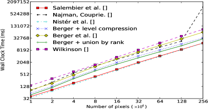
(a)

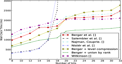
(b)

Figure 4: (a) Comparison of algorithms on a 8-bit image as a function of size; (b) Comparison of algorithms on a 6 Mega-pixels image as a function of quantization.

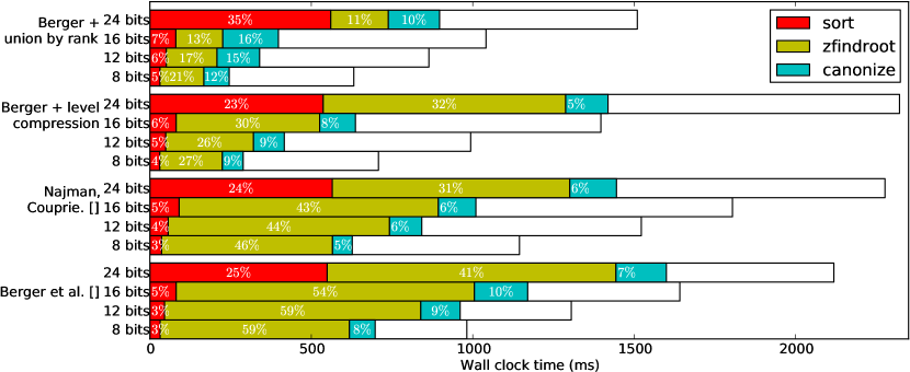
Figure 5: Time spent in each part of the sequential version of union-find based algorithms.

Benchmark were performed on an Intel Core i7 (4 physical cores, 8 logical cores). Program have been compiled with gcc 4.7, optimization flags on (--O3 --march=native). Tests have been conducted on a 6MB 8-bit image. Image has been resized by cropping or tiling the original image and over-quantization has been performed by shifting the eight bits left and generating missing lower bits at random. Figure 4 evaluates performance of sequential algorithms w.r.t to image size and quantization. A first remark, we notice that all algorithms are linear in practice. On natural image, the upper bound $n\log n$ complexity of Wilkinson [20] and Berger et al. [2] algorithms is not reached. Let start with union-find based algorithms. Berger et al. [2] and Najman and Couprie [10] have quite the same running time ($\pm 6\%$ on average), however performances of Najman and Couprie [10] algorithm drops significantly at 256 Mega-pixels. Indeed, at that size each auxiliary array/image requires 1 GB memory space, thus Najman and Couprie [10] that uses much memory exceeds the 6 GB RAM limit and needs to swap with the hard drive. Our implementation of union-by-rank uses less memory and is on average $42\%$ faster than Najman and Couprie [10]. Level compression is an efficient optimization that provides $35\%$ speed up on average on Berger et al. [2]. However, this optimization is only reliable on low quantized data, figure 4b shows that it is relevant until 18 bits. Since it operates on flat-zones, when quantization gets higher flat-zones are less probable, thus time saved in findroot to find canonical elements does not balance extra tests overheads (see Figure 5. Union-find is not affected by the quantization but sorting does, counting sort and radix sort complexities are respectively linear and logarithmic with the number of bits. The break in union-find curves between 18 and 20 bits stands for the switch from counting to radix sort. Flooding-based algorithms using hierarchical queues outperform our union-find by rank on low quantized image by $41\%$ on average. As expected Salembier et al. [13] and Nistér and Stewénius [11] (which is the exact non-recursive version of the first one) closely match. However, the exponential cost of hierarchical queues w.r.t the number of bits is evident on figure 4b. By using a standard heap instead of hierarchical queues, Wilkinson [20] does scale well with the number of bits and outperform every algorithms except our implementation of union-by-rank. In [20], the algorithm is supposed to match Salembier et al. [13]’s method for low quantized images, but in our experiment it stays 4 times slower. As a consequence:

• since Najman and Couprie [10]’s algorithm is always outperformed by our implementation of union-find by rank, it will not be tested any further.

• [11] and [20] are merged in our single implementation (called Non-recursive Salembier below) that will use hierarchical queues for heap when quantization is below 18 and switches to a standard heap implementation otherwise.

• the algorithm Berger + level compression will enable level compression only when quantization is below 18 bits.

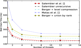
(a)

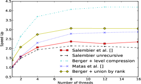
(b)

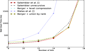
(c)

Figure 6: (a,b) Comparison of parallel algorithms on a 6 Mega-pixels 8-bits image as a function of number of threads; (a) Wall clock time; (b) Speed up w.r.t the sequential version; (c) Comparison of parallel algorithms on a 6 Mega-pixels image as a function of quantization.

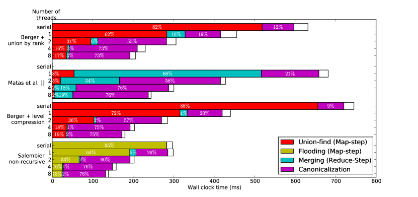
Figure 7: Time spent in each part of parallel versions of algorithms.

Figure 6 shows results of the map-reduce idiom applied on many algorithms and their parallelism. As a first result, we can see best performance are generally achieve with 8 threads that is when the number of thread matches the number of (logical) cores. However, since there are actually only 4 physical cores, we can expect a $\times 4$ maximum speed up. Some algorithms take more benefits from map-reduce than others. Union-find based are algorithms are particularly well-suited for parallelism, union-find with level compression achieves the best speed up ($\times 4.2$) at 12 threads and union-find by rank a $\times 3.1$ speed up with 8 threads. More surprising, map-reduce pattern achieves significant speed up even when a single thread is used (respectively $\times 1.7$ and $\times 1.4$ for union-find with level compression and union-find by rank). This result that used to surprise Wilkinson et al. [19] as well is explained by a better cache coherence when working on sub-domains that balances tree merges overhead. On the other hand, flooding algorithms do not scale as well because they are limited by the canonization and $S$ reconstruction post-process (that is going to happen also for union-find algorithms on architecture with more cores). In [19] and [6], they obtain a speed up almost linear with the number of threads because only a $parent$ image is built. If we remove canonization and $S$ construction step, we also get those speed ups.(). Figure 6c shows the exponential complexity of merging trees as number of bits increases that makes parallel algorithms unsuitable for high quantized data. In the light of the previous analysis, Figure 8 provides guidelines to choose the right max-tree algorithm w.r.t to image types and architectures.

Figure 8: Decision tree to choose the right max-tree algorithm

5 Conclusion

In this paper, we have tried to lead a fair comparison of max-tree algorithms in a unique framework. We have highlighted the fact that there is no best algorithm that supersedes all the others in every cases and eventually we have given a decision tree to choose the right algorithm w.r.t to data and hardware. We have proposed a max-tree algorithm using union-by-rank that outperforms the existing one from [10]. Furthermore, we have proposed a second one that uses level compression for systems with strict memory constraints. As further work, we shall include image contents as a new parameter of comparison, for instance images with large flat zones (e.g. cartoons) or images having strongly non-uniform distribution of gray levels. A code intensively tested used for these benachmarks is available on the Internet at http://www.lrde.epita.fr/cgi-bin/twiki/view/Olena/maxtree.

References

- Andersson et al. [1995] Andersson, A., Hagerup, T., Nilsson, S., Raman, R.: Sorting in linear time? In: Proc. of the Annual ACM symposium on Theory of computing. pp. 427–436 (1995)
- Berger et al. [2007] Berger, C., Géraud, T., Levillain, R., Widynski, N., Baillard, A., Bertin, E.: Effective component tree computation with application to pattern recognition in astronomical imaging. In: Proc. of ICIP. vol. 4, pp. IV–41 (2007)
- Hesselink [2003] Hesselink, W.: Salembier’s min-tree algorithm turned into breadth first search. Information processing letters 88(5), 225–229 (2003)
- Jones [1999] Jones, R.: Connected filtering and segmentation using component trees. Computer Vision and Image Understanding 75(3), 215–228 (1999)
- Matas et al. [2004] Matas, J., Chum, O., Urban, M., Pajdla, T.: Robust wide-baseline stereo from maximally stable extremal regions. IVC 22(10), 761–767 (2004)
- Matas et al. [2008] Matas, P., Dokladalova, E., Akil, M., Grandpierre, T., Najman, L., Poupa, M., Georgiev, V.: Parallel algorithm for concurrent computation of connected component tree. In: Advanced Concepts for Intelligent Vis. Sys. pp. 230–241 (2008)
- Meijster et al. [2002] Meijster, A., Westenberg, M., Wilkinson, M.: Interactive shape preserving filtering and visualization of volumetric data. In: Proc. of ISIP. pp. 640–643 (2002)
- Menotti et al. [2007] Menotti, D., Najman, L., de Albuquerque Araújo, A.: 1d component tree in linear time and space and its application to gray-level image multithresholding. In: Proc. of ISMM. pp. 437–448 (2007)
- Monasse and Guichard [2000] Monasse, P., Guichard, F.: Fast computation of a contrast-invariant image representation. IEEE Trans. on Ima. Proc. 9(5), 860–872 (2000)
- Najman and Couprie [2006] Najman, L., Couprie, M.: Building the component tree in quasi-linear time. IEEE Trans. on Ima. Proc. 15(11), 3531–3539 (2006)
- Nistér and Stewénius [2008] Nistér, D., Stewénius, H.: Linear time maximally stable extremal regions. In: Proc. of ECCV. pp. 183–196 (2008)
- Perret et al. [2010] Perret, B., Lefevre, S., Collet, C., Slezak, É.: Connected component trees for multivariate image processing and applications in astronomy. In: Proc. of ICPR. pp. 4089–4092 (2010)
- Salembier et al. [1998] Salembier, P., Oliveras, A., Garrido, L.: Antiextensive connected operators for image and sequence processing. IEEE Trans. on Ima. Proc. 7(4), 555–570 (1998)
- Salembier and Serra [1995] Salembier, P., Serra, J.: Flat zones filtering, connected operators, and filters by reconstruction. IEEE Trans. on Ima. Proc. 4(8), 1153–1160 (1995)
- Tarjan [1975] Tarjan, R.: Efficiency of a good but not linear set union algorithm. JACM 22(2), 215–225 (1975)
- Urbach and Wilkinson [2002] Urbach, E., Wilkinson, M.: Shape-only granulometries and grey-scale shape filters. In: Proc. of ISMM. vol. 2002, pp. 305–314 (2002)
- Vincent [1993] Vincent, L.: Grayscale area openings and closings, their efficient implementation and applications. In: Proc. of EURASIP Workshop on Mathematical Morphology and its Applications to Signal Processing. pp. 22–27 (1993)
- Wilkinson and Westenberg [2001] Wilkinson, M., Westenberg, M.: Shape preserving filament enhancement filtering. In: Proc. of MICCAI. pp. 770–777 (2001)
- Wilkinson et al. [2008] Wilkinson, M., Gao, H., Hesselink, W., Jonker, J., Meijster, A.: Concurrent computation of attribute filters on shared memory parallel machines. PAMI 30(10), 1800–1813 (2008)
- Wilkinson [2011] Wilkinson, M.H.F.: A fast component-tree algorithm for high dynamic-range images and second generation connectivity. In: Proc. of ICIP. pp. 1021–1024 (2011)
- Xu et al. [2012] Xu, Y., Géraud, T., Najman, L., et al.: Morphological filtering in shape spaces: Applications using tree-based image representations. In: Proc. of ICPR. pp. 1–4 (2012)