Virial mass in warped DGP-inspired ${\cal L}(R)$ gravity

Abstract

A version of the virial theorem is derived in a brane-world scenario in the framework of a warped DGP model where the action on the brane is an arbitrary function of the Ricci scalar, ${\cal L}(R)$. The extra terms in the modified Einstein equations generate an equivalent mass term (geometrical mass), which give an effective contribution to the gravitational energy and offer viable explanation to account for the virial mass discrepancy in clusters of galaxies. We also obtain the radial velocity dispersion of galaxy clusters and show that it is compatible with the radial velocity dispersion profile of such clusters. Finally, we compare the result of the model with ${\cal L}(R)$ gravity theories.
PACS numbers: 04.50.-h, 04.20.Jb, 04.20.Cv, 95.35.+d
Key words: Virial mass, DGP brane-world, Boltzmann equation, Radial velocity dispersion.

1 Introduction

The intriguing possibility that our universe is only part of a higher dimensional space-time has raised a lot of interest in the physics community [1], motivated by the developments in superstring and M-theory. According to the brane-world scenario, all matter and gauge interactions reside on the brane, while gravity can propagate in the whole five-dimensional space time (figure 1) [2]. Higher dimensional models have a long history, but it revived by works of Randall and Sundrum (RS) in 1999 [3]. They have introduced two models in order to solve the hierarchy problem in particle physics, however after a while these two models, because of their interesting properties, could attract a salient attention in cosmology. In their first model they suppose two brane which our brane has a negative tension (Shiromizu et al. [4] have shown that this model is unphysical). In their second model they suppose a brane with infinite extra dimension. In that model our universe has a positive tension. The effective four-dimensional gravity in the brane is modified by extra dimension. The cosmological evolution of such a brane universe has been extensively investigated and effects such as a quadratic density term in the Friedmann equations have been found [5, 6, 7]. An alternative scenario was subsequently proposed by Dvali, Gabadadze and Porrati (DGP) [8]. The DGP proposal rests on the key assumption of the presence of a four-dimensional Ricci scalar in the brane action. There are two main reasons that make this model phenomenologically appealing. First, it predicts that four-dimensional Newtonian gravity on a brane-world is regained at distances shorter than a given crossover scale $r_{c}$ (high energy limit), whereas five-dimensional effects become manifest above that scale (low energy limit) [9]. Second, the model can explain late-time acceleration without having to invoke a cosmological constant or quintessential matter [10]. An extension of the DGP brane-world scenario have been constructed by Maeda, Mizuno and Torii which is the combination of the RS II model and DGP model [11]. In this combination, an induced curvature term appears on the brane in the RS II model which has been called the warped DGP brane-world in literature [12]. In this paper, we consider the effective gravitational field equations within the context of the warped DGP brane-world model where the action on the brane is an arbitrary function of the Ricci scalar, ${\cal L}(R)$, (which is called the modified DGP brane-world model in this work) and obtain the spherically symmetric equations in this scenario. For a recent and comprehensive review of the phenomenology of DGP cosmology, the reader is referred to [13].

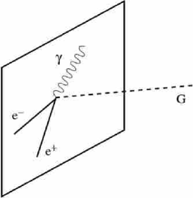
Figure 1: The confinement of matter to the brane, while gravity propagates in the bulk.

In the past two decades, various attempts have been made to understand the nature of the so called dark energy and dark matter which would be required to explain many observational data. The question of dark matter is presently one of the most intriguing aspects in astrophysics and cosmology. There are some compelling observational evidence for the existence of dark matter for which, the galaxy rotation curves and mass discrepancy in cluster of galaxies are two prominent examples [14]. Galaxy clusters are the largest virialized structures in the universe, and their mass content is supposed to be representative of the universe as a whole. The total mass of galaxy clusters can be determined in a variety of ways. The application of the virial theorem to positions and velocities of cluster member galaxies is the oldest method of cluster mass determination [15]. More recent methods are based on the dynamical analysis of hot x-ray emitting gas [16] and on the gravitational lensing of background galaxies [17]. The mass determined from such dynamical means is always found to be in excess of that which can be attributed to the visible matter. This is known as the missing mass problem. The existence of dark matter was not firmly established until the measurement of the rotational velocity of stars and gases orbiting at a distance $r$ from the galactic center could be done with reasonable accuracy. Observations show that the rotational velocity increases near the center of a galaxy and approaches a nearly constant value with increasing distance from the center. The discrepancy between the observed rotational velocity curves and the theoretical prediction from Newtonian mechanics is known as the galactic rotation curves problem (figure 2). This discrepancy is explained by postulating that every galaxy and cluster of galaxies is embedded in a halo made up of some dark matter. To deal with the question of dark matter, a great number of efforts has been concentrated on various modifications to the Newtonian gravity or general relativity [18, 19, 20]. There are also geometrical approaches to address this problem, namely to use modified Einstein field equations, as is done in brane-world models [21, 22, 23, 24] or in modified gravity theories [25, 26].

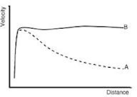
Figure 2: Observed rotation velocity curve (solid line B) and the prediction from Newtonian theory (dotted line A).

In what follows, we first give a brief review of warped DGP brane-world inspired by the ${\cal L}(R)$ term [27]. Next, we introduce the relativistic collision-less Boltzmann equation from which we deduce the generalized virial theorem with the aid of the modified Einstein field equations. The geometric mass and density of a cluster is then identified in terms of the observable quantities. Then we derive the radial velocity dispersion relation in galaxies. Finally, in the last section, we discuss and conclude on our results.

2 Einstein equations in warped DGP brane-${\cal L}(R)$ model

We are going to obtain the relativistic virial theorem for galaxy clusters in warped DGP brane-${\cal L}(R)$ model. For this end we need, as a first step, to obtain the gravitational field equations. Consider a 3-brane $\Sigma$ embedded in a five-dimensional bulk ${\cal M}$. The effective action of a warped DGP-inspired ${\cal L}(R)$ scenario is given by

$${\cal S}={\cal S}_{bulk}+{\cal S}_{brane},$$ (1)

where

$${\cal S}_{bulk}=\int_{{\cal M}}d^{5}X\sqrt{-{\cal G}}\left[\frac{1}{2\kappa_{5}^{2}}{\cal R}+{\cal L}_{m}^{(5)}\right],$$ (2)

$${\cal S}_{brane}=\int_{\Sigma}d^{4}x\sqrt{-g}{\cal L}_{brane}(g_{\alpha\beta},\psi)+\int_{\Sigma}d^{4}x\sqrt{-g}\frac{K^{\pm}}{\kappa_{5}^{2}}.$$ (3)

Here, $X^{A}$, ($A=0,1,2,3,4$) are five-dimensional coordinates, while $x^{\mu}$, ($\mu=0,1,2,3$) are the induced four-dimensional coordinates on the brane. $\kappa_{5}^{2}=8\pi G_{5}$ is the five-dimensional gravitational constant, ${\cal R}$ and ${\cal L}_{m}^{(5)}$ are the five-dimensional scalar curvature and the matter Lagrangian in the bulk, respectively. $K=\nabla_{\mu}n^{\mu}$ is the trace of extrinsic curvature on either side of the brane where $n_{\mu}$ is the unit vecror perpendicular to the brane hypersurface $\Sigma$ [28]. The last term in equation (3) is known as the York-Gibbons-Hawking term which provides a through framework for imposing suitable boundary conditions on the field equations. ${\cal L}_{brane}(g_{\alpha\beta},\psi)$ is the effective four-dimensional Lagrangian, which is given by a generic functional of the brane metric $g_{\alpha\beta}$ and matter fields.

The five-dimensional Einstein field equations are given by

$${\cal R}_{AB}-\frac{1}{2}{\cal R}{\cal G}_{AB}={\kappa_{5}^{2}}\left[T^{(5)}_{AB}+\delta(Y)\tau_{AB}\right],$$ (4)

where

$$T^{(5)}_{AB}\equiv-2\frac{\delta{\cal L}^{(5)}_{m}}{\delta{\cal G}^{AB}}+{\cal G}_{AB}{\cal L}^{(5)}_{m},$$ (5)

and

$$\tau_{\mu\nu}\equiv-2\frac{\delta{\cal L}_{brane}}{\delta g^{\mu\nu}}+g_{\mu\nu}{\cal L}_{brane}.$$ (6)

We study the case where the induced gravity scenario arises from higher-order corrections on the scalar curvature over the brane. The interaction between the bulk gravity and local matter induces gravity on the brane through its quantum effects. If we take into account quantum effects of the matter fields confined to the brane, the gravitational action on the brane is modified as

$${\cal L}_{brane}(g_{\alpha\beta},\psi)=\frac{\mu^{2}}{2}{\cal L}(R)-\lambda_{b}+{\cal L}_{m},$$ (7)

where $\mu$ is a mass scale which may correspond to the four-dimensional Planck mass, $\lambda_{b}$ is the tension of the brane and ${\cal L}_{m}$ presents the Lagrangian of the matter fields on the brane. We note that for ${\cal L}(R)=R$, action (1) gives the DGP model if $\lambda_{b}=\Lambda^{(5)}=0$ and gives the RSII model if $\mu=0$.

We obtain the gravitational field equations on the brane-world as [4]

$$G_{\mu\nu}=\frac{2\kappa_{5}^{2}}{3}\left[T_{AB}^{(5)}g^{A}_{\mu}g^{B}_{\nu}+g_{\mu\nu}\left(T_{AB}^{(5)}n^{A}n^{B}-\frac{1}{4}T^{(5)}\right)\right]+\kappa_{5}^{4}\pi_{\mu\nu}-{\cal E}_{\mu\nu},$$ (8)

where the quadratic correction has the form

$$\pi_{\mu\nu}=-\frac{1}{4}\tau_{\mu\alpha}\tau_{\nu}^{\alpha}+\frac{1}{12}\tau\tau_{\mu\nu}+\frac{1}{8}g_{\mu\nu}\tau^{\alpha\beta}\tau_{\alpha\beta}-\frac{1}{24}g_{\mu\nu}\tau^{2},$$ (9)

and

$${\cal E}_{\mu\nu}=C^{(5)}_{ABCD}n^{A}n^{B}g^{C}_{\,\,\,\mu}g^{D}_{\,\,\,\nu},$$ (10)

is the projection of the bulk Weyl tensor to the surface orthogonal to $n^{A}$. By the variation over the metric, we can also obtain the surface equation as

$$\kappa_{5}^{2}\tau_{\mu\nu}=K_{\mu\nu}-Kg_{\mu\nu},$$ (11)

where $K_{\mu\nu}$ is the extrinsic curvature and $\tau_{\mu\nu}$ is the total energy-momentum tensor of the brane. Equation (11) is nothing but the Israel junction condition [29]. By taking the divergence of the Israel equation, we have

$$\kappa_{5}^{2}\nabla_{\mu}\tau^{\mu\nu}=\nabla_{\mu}K^{\mu\nu}-g^{\mu\nu}\nabla_{\mu}K,$$ (12)

where $\nabla_{\mu}$ is the covariant derivative with respect to $g_{\mu\nu}$. The right hand side can be evaluated using Codacci’s equation and the field equation of the bulk, giving

$$\nabla_{\nu}\tau_{\mu}^{\nu}=-2T_{AB}^{(5)}n^{A}g^{B}_{\mu}.$$ (13)

Also, we note that the junction conditions are ambiguous and do not define the four-dimensional geometry in the unique way. If one changes the surface action (freedom in the choice of boundary terms), the junction condition (11) is also changed. This shows that brane-world is lacking the physical principle to predict in unique way the surface term and, hence, the emerging brane cosmology [30]. One may prescribe the AdS/CFT correspondence to define the boundary action [31] where curvature surface terms correspond to usual counterterms in dual QFT.

In order to find the basic field equations on the brane with induced gravity described by ${\cal L}(R)$ term, we have to obtain the energy-momentum tensor of the brane $\tau_{\mu\nu}$ by definition (6) from Lagrangian (7), yielding

$$\tau_{\mu\nu}=-\Lambda(R)g_{\mu\nu}+T_{\mu\nu}-\Sigma(R)G_{\mu\nu}+\Theta_{\mu\nu},$$ (14)

where the functions $\Lambda(R)$, $\Sigma(R)$ and $\Theta_{\mu\nu}$ are defined as

$$\Lambda(R)=\frac{\mu^{2}}{2}\left[R\frac{d{\cal L}(R)}{dR}-{\cal L}(R)+2\frac{\lambda_{b}}{\mu^{2}}\right],$$ (15)

$$\Sigma(R)=\mu^{2}\frac{d{\cal L}(R)}{dR},$$ (16)

and

$$\Theta_{\mu\nu}=\mu^{2}\left[\nabla_{\mu}\nabla_{\nu}{\left(\frac{d{\cal L}(R)}{dR}\right)}-g_{\mu\nu}\nabla^{\beta}\nabla_{\beta}\left(\frac{d{\cal L}(R)}{dR}\right)\right].$$ (17)

Inserting equations (14) into equation (8), we find the effective field equations for the four-dimensional metric $g_{\mu\nu}$ as [27]

$$\left[1+\frac{1}{6}\kappa_{5}^{4}\Lambda(R)\Sigma(R)\right]G_{\mu\nu}=\frac{1}{6}\kappa_{5}^{4}\Lambda(R)T_{\mu\nu}-\Lambda_{4}(R)g_{\mu\nu}+\frac{1}{6}\kappa_{5}^{4}\Lambda(R)\Theta_{\mu\nu}+\kappa_{5}^{4}\pi_{\mu\nu}^{(T)}+\kappa_{5}^{4}\pi_{\mu\nu}^{(\Theta)}$$ (18)

$$+ \kappa_{5}^{4}\Sigma(R)^{2}\pi_{\mu\nu}^{(G)}-\kappa_{5}^{4}\Sigma(R){K}^{(T)}_{\mu\nu\rho\sigma}G^{\rho\sigma}-\kappa_{5}^{4}\left[\Sigma(R)G^{\rho\sigma}-T^{\rho\sigma}\right]{K}^{(\Theta)}_{\mu\nu\rho\sigma}-{\cal E}_{\mu\nu},$$

where

$$\pi^{(T)}_{\mu\nu}=-\frac{1}{4}T_{\mu\alpha}T^{\alpha}_{\nu}+\frac{1}{12}TT_{\mu\nu}+\frac{1}{8}g_{\mu\nu}T_{\alpha\beta}T^{\alpha\beta}-\frac{1}{24}g_{\mu\nu}T^{2},$$ (19)

$$\pi^{(G)}_{\mu\nu}=-\frac{1}{4}G_{\mu\alpha}G^{\alpha}_{\nu}+\frac{1}{12}GG_{\mu\nu}+\frac{1}{8}g_{\mu\nu}G_{\alpha\beta}G^{\alpha\beta}-\frac{1}{24}g_{\mu\nu}G^{2},$$ (20)

$$\pi^{(\Theta)}_{\mu\nu}=-\frac{1}{4}\Theta_{\mu\alpha}\Theta^{\alpha}_{\nu}+\frac{1}{12}\Theta\Theta_{\mu\nu}+\frac{1}{8}g_{\mu\nu}\Theta_{\alpha\beta}\Theta^{\alpha\beta}-\frac{1}{24}g_{\mu\nu}\Theta^{2},$$ (21)

and

$${K}^{(T)}_{\mu\nu\rho\sigma}=\frac{1}{4}\left(g_{\mu\nu}T_{\rho\sigma}-g_{\mu\rho}T_{\nu\sigma}-g_{\nu\sigma}T_{\mu\rho}\right)+\frac{1}{12}\left[T_{\mu\nu}g_{\rho\sigma}+T(g_{\mu\rho}g_{\nu\sigma}-g_{\mu\nu}g_{\rho\sigma})\right],$$ (22)

$${K}^{(\Theta)}_{\mu\nu\rho\sigma}=\frac{1}{4}\left(g_{\mu\nu}\Theta_{\rho\sigma}-g_{\mu\rho}\Theta_{\nu\sigma}-g_{\nu\sigma}\Theta_{\mu\rho}\right)+\frac{1}{12}\left[\Theta_{\mu\nu}g_{\rho\sigma}+\Theta(g_{\mu\rho}g_{\nu\sigma}-g_{\mu\nu}g_{\rho\sigma})\right],$$ (23)

with $T$ being the trace of the energy-momentum tensor and $\Theta$ is

$$\Theta=g^{\mu\nu}\Theta_{\mu\nu}=-3\mu^{2}\nabla^{\alpha}\nabla_{\alpha}\left(\frac{d{\cal L}(R)}{dR}\right),$$ (24)

and the effective cosmological constant on the brane is given by

$$\Lambda_{4}(R)=\frac{1}{2}\kappa_{5}^{2}\left[\Lambda^{(5)}+\frac{1}{6}\kappa_{5}^{2}\Lambda(R)^{2}\right].$$ (25)

We can also recover the standard four-dimensional ${\cal L}(R)$ gravity [32] from equation (18) in the limit $\lambda_{b}^{-1}\rightarrow 0$. A alternative possibility in recovering the four-dimensional ${\cal L}(R)$ gravity is to take the limit $\kappa_{5}\rightarrow 0$, while keeping the Newtonian gravitational constant $\kappa_{4}^{2}$ finite [4] (see Appendix A).

Now we are interested in computing the spherically symmetric solutions on the brane. We consider an isolated and spherically symmetric cluster being described by a static and spherically symmetric metric

$$ds^{2}=-e^{\lambda(r)}dt^{2}+e^{\nu(r)}dr^{2}+r^{2}(d\theta^{2}+sin^{2}\theta d\varphi^{2}),$$ (26)

we also assume that the matter content of the bulk is just a cosmological constant $\Lambda^{(5)}$ and the matter content of the 3-brane universe is considered to be a cosmological constant plus a localized spherically symmetric perfect fluid

$$T_{\mu\nu}=(p_{b}+\rho_{b})v_{\mu}v_{\nu}+p_{b}g_{\mu\nu}.$$

Therefore, the gravitational field equations become

$$\left[1+\frac{1}{6}\kappa_{5}^{4}\Lambda(R)\Sigma(R)\right]\frac{e^{-\nu}}{r^{2}}\left(-1+r\nu^{{}^{\prime}}+e^{\nu}\right)=\frac{1}{6}\kappa_{5}^{4}\Lambda(R)\rho_{b}+\Lambda_{4}(R)-\frac{1}{6}\kappa_{5}^{4}\Lambda(R)\Theta_{0}^{0}+\frac{\kappa_{5}^{4}}{12}\rho_{b}^{2}$$ (27)

$$+ \kappa_{5}^{4}\Sigma(R){\cal K}_{0}^{0(T)}-\kappa_{5}^{4}\Sigma(R)^{2}\pi_{0}^{0(G)}-\kappa_{5}^{4}{\cal K}_{0}^{0(\Theta)}+\kappa_{5}^{4}\Sigma(R){\cal K}_{0}^{0(G)}-\kappa_{5}^{4}\pi_{0}^{0(\Theta)}+\frac{6}{\kappa_{4}^{2}\lambda_{b}}U(r),$$

$$\left[1+\frac{1}{6}\kappa_{5}^{4}\Lambda(R)\Sigma(R)\right]\frac{e^{-\nu}}{r^{2}}\left(1+r\lambda^{{}^{\prime}}-e^{\nu}\right)=\frac{1}{6}\kappa_{5}^{4}\Lambda(R)p_{b}-\Lambda_{4}(R)+\frac{1}{6}\kappa_{5}^{4}\Lambda(R)\Theta_{1}^{1}+\frac{\kappa_{5}^{4}}{12}\left(\rho_{b}^{2}+2\rho_{b}p_{b}\right)$$ (28)

$$- \kappa_{5}^{4}\Sigma(R){\cal K}_{1}^{1(T)}+\kappa_{5}^{4}\Sigma(R)^{2}\pi_{1}^{1(G)}+\kappa_{5}^{4}{\cal K}_{1}^{1(\Theta)}-\kappa_{5}^{4}\Sigma(R){\cal K}_{1}^{1(G)}+\kappa_{5}^{4}\pi_{1}^{1(\Theta)}+\frac{2}{\kappa_{4}^{2}\lambda_{b}}\left[U(r)+2P(r)\right],$$

$$\left[1+\frac{1}{6}\kappa_{5}^{4}\Lambda(R)\Sigma(R)\right]\frac{e^{-\nu}}{2r}\left(2\lambda^{{}^{\prime}}-2\nu^{{}^{\prime}}-\lambda^{{}^{\prime}}\nu^{{}^{\prime}}r+2\lambda^{{}^{\prime\prime}}r+\lambda^{{}^{\prime}2}r\right)=\frac{1}{3}\kappa_{5}^{4}\Lambda(R)p_{b}-2\Lambda_{4}(R)+\frac{1}{3}\kappa_{5}^{4}\Lambda(R)\Theta_{2}^{2}$$ (29)

$$+ \frac{\kappa_{5}^{4}}{6}\left(\rho_{b}^{2}+2\rho_{b}p_{b}\right)-2\kappa_{5}^{4}\Sigma(R){\cal K}_{2}^{2(T)}+2\kappa_{5}^{4}\Sigma(R)^{2}\pi_{2}^{2(G)}+2\kappa_{5}^{4}{\cal K}_{2}^{2(\Theta)}-2\kappa_{5}^{4}\Sigma(R){\cal K}_{2}^{2(G)}$$

$$+ 2\kappa_{5}^{4}\pi_{2}^{2(\Theta)}+\frac{4}{\kappa_{4}^{2}\lambda_{b}}[U(r)-P(r)],$$

where $U(r)$ and $P(r)$ are the dark radiation and dark pressure. Also ${\cal K}_{\mu\nu}^{(T)}$, ${\cal K}_{\mu\nu}^{(G)}$ and ${\cal K}_{\mu\nu}^{(\Theta)}$ are defined as

$${K}_{\mu\nu\rho\sigma}^{(T)}G^{\rho\sigma}\equiv{\cal K}_{\mu\nu}^{(T)},$$

$${K}_{\mu\nu\rho\sigma}^{(\Theta)}G^{\rho\sigma}\equiv{\cal K}_{\mu\nu}^{(G)},$$

$${K}_{\mu\nu\rho\sigma}^{(\Theta)}T^{\rho\sigma}\equiv{\cal K}_{\mu\nu}^{(\Theta)}.$$

Now, using these relations and adding the gravitational field equations (27)-(29) we find

$$\left(1+\frac{1}{6}\kappa_{5}^{4}\Lambda(R)\Sigma(R)\right)e^{-\nu}\left(\frac{\lambda^{{}^{\prime}}}{r}-\frac{\lambda^{{}^{\prime}}\nu^{{}^{\prime}}}{4}+\frac{\lambda^{{}^{\prime\prime}}}{2}+\frac{\lambda^{{}^{\prime}2}}{4}\right)=\frac{\kappa_{5}^{4}}{12}\Lambda(R)\left(\rho_{b}+3p_{b}\right)-\Lambda_{4}(R)+\frac{\kappa_{5}^{4}}{12}\rho_{b}(2\rho_{b}+3p_{b})$$ (30)

$$- \frac{1}{12}\kappa_{5}^{4}\Lambda(R)[\Theta_{0}^{0}-\Theta_{1}^{1}-2\Theta_{2}^{2}]+\frac{\kappa_{5}^{4}\Sigma(R)}{2}[{\cal K}_{0}^{0(T)}-{\cal K}_{1}^{1(T)}-2{\cal K}_{2}^{2(T)}]+\frac{\kappa_{5}^{4}\Sigma(R)}{2}[{\cal K}_{0}^{0(G)}-{\cal K}_{1}^{1(G)}-2{\cal K}_{2}^{2(G)}]$$

$$- \frac{\kappa_{5}^{4}}{2}[{\cal K}_{0}^{0(\Theta)}-{\cal K}_{1}^{1(\Theta)}-2{\cal K}_{2}^{2(\Theta)}]-\frac{\kappa_{5}^{4}\Sigma(R)^{2}}{2}[\pi_{0}^{0(G)}-\pi_{1}^{1(G)}-2\pi_{2}^{2(G)}]$$

$$- \frac{\kappa_{5}^{4}}{2}[\pi_{0}^{0(\Theta)}-\pi_{1}^{1(\Theta)}-2\pi_{2}^{2(\Theta)}]+\frac{6}{\kappa_{4}^{2}\lambda_{b}}U(r),$$

where

$${\cal K}_{0}^{0(T)}-{\cal K}_{1}^{1(T)}-2{\cal K}_{2}^{2(T)} = \frac{1}{12}e^{-\nu}[\frac{6\rho_{b}}{r^{2}}(1-e^{\nu})+\frac{6p_{b}}{r^{2}}(1-e^{\nu})-\frac{4p_{b}\nu^{\prime}}{r}+\rho_{b}\lambda^{\prime}\nu^{\prime}-2\rho_{b}\lambda^{\prime\prime}-\rho_{b}\lambda^{\prime 2}$$ (31)

$$- \frac{4\rho_{b}\lambda^{\prime}}{r}-\frac{2p_{b}\nu^{\prime}}{r}-\frac{6\rho_{b}\nu^{\prime}}{r}],$$

$${\cal K}_{0}^{0(G)}-{\cal K}_{1}^{1(G)}-2{\cal K}_{2}^{2(G)} = \frac{\mu^{2}}{24}e^{-\nu}\left[(\frac{6\lambda^{\prime}}{r^{2}}+\frac{2\nu^{\prime}}{r^{2}}-\frac{8}{r^{3}})R^{\prime}\frac{d^{2}{\cal L}}{dR^{2}}-\frac{4}{r^{2}}R^{\prime\prime}\frac{d^{2}{\cal L}}{dR^{2}}-\frac{4}{r^{2}}R^{\prime 2}\frac{d^{3}{\cal L}}{dR^{3}}\right]$$ (32)

$$- \frac{\mu^{2}}{24}e^{-2\nu}\{(-\frac{8}{r^{3}}+\frac{10\nu^{\prime}}{r^{2}}-{\nu^{\prime}\lambda^{\prime 2}}-\frac{14\nu^{\prime}\lambda^{\prime}}{r}+\frac{8\lambda^{\prime\prime}}{r}+\lambda^{\prime}\nu^{\prime 2}+\frac{22\lambda^{\prime}}{r^{2}}+\frac{4\lambda^{\prime 2}}{r}$$

$$- 2\nu^{\prime}\lambda^{\prime\prime}-\frac{2\nu^{\prime 2}}{r})R^{\prime}\frac{d^{2}{\cal L}}{dR^{2}}+(2\lambda^{\prime 2}-\frac{4}{r^{2}}+\frac{8\lambda^{\prime}}{r}+\frac{4\nu^{\prime}}{r}-2\lambda^{\prime}\nu^{\prime}+4\lambda^{\prime\prime})R^{\prime\prime}\frac{d^{2}{\cal L}}{dR^{2}}$$

$$+ (\frac{4\nu^{\prime}}{r}+\frac{8\lambda^{\prime}}{r}-2\lambda^{\prime}\nu^{\prime}+2\lambda^{\prime 2}-\frac{4}{r^{2}}+4\lambda^{\prime\prime})R^{\prime 2}\frac{d^{3}{\cal L}}{dR^{3}}\},$$

$${\cal K}_{0}^{0(\Theta)}-{\cal K}_{1}^{1(\Theta)}-2{\cal K}_{2}^{2(\Theta)} = -\frac{1}{12}\mu^{2}e^{-\nu}[\frac{4}{r}(2\rho_{b}+3p_{b})R^{\prime}\frac{d^{2}{\cal L}}{dR^{2}}-(2\rho_{b}+3p_{b})\nu^{\prime}R^{\prime}\frac{d^{2}{\cal L}}{dR^{2}}-3\rho_{b}\lambda^{\prime}R^{\prime}\frac{d^{2}{\cal L}}{dR^{2}}$$ (33)

$$+ 2(2\rho_{b}+3p_{b})R^{\prime\prime}\frac{d^{2}{\cal L}}{dR^{2}}+2(2\rho_{b}+3p_{b})R^{\prime 2}\frac{d^{3}{\cal L}}{dR^{3}}],$$

and

$$\pi_{0}^{0(G)}-\pi_{1}^{1(G)}-2\pi_{2}^{2(G)} = -\frac{1}{12}e^{-2\nu}[\frac{2\nu^{\prime}\lambda^{\prime\prime}}{r}+\frac{\lambda^{\prime 2}\nu^{\prime}}{r}+\frac{5\lambda^{\prime}\nu^{\prime}}{r^{2}}-\frac{\lambda^{\prime}\nu^{\prime 2}}{r}+\frac{2}{r^{4}}-\frac{4\nu^{\prime}}{r^{3}}-\frac{\lambda^{\prime 2}}{r^{2}}-\frac{4\lambda^{\prime}}{r^{3}}-\frac{2\lambda^{\prime\prime}}{r^{2}}$$ (34)

$$+ \frac{2\nu^{\prime 2}}{r^{2}}]-\frac{1}{12}e^{-\nu}[\frac{4\lambda^{\prime}}{r^{3}}+\frac{4\nu^{\prime}}{r^{3}}+\frac{\lambda^{\prime 2}}{r^{2}}+\frac{2\lambda^{\prime\prime}}{r^{2}}-\frac{4}{r^{4}}-\frac{\lambda^{\prime}\nu^{\prime}}{r^{2}}+\frac{2e^{\nu}}{r^{4}}],$$

$${\pi}_{0}^{0(\Theta)}-{\pi}_{1}^{1(\Theta)}-2{\pi}_{2}^{2(\Theta)}=\frac{1}{8}e^{-2\nu}\mu^{4}R^{\prime}\lambda^{\prime}\frac{d^{2}{\cal L}}{dR^{2}}\left[(2R^{\prime\prime}-\nu^{\prime}R^{\prime}+\frac{4R^{\prime}}{r})\frac{d^{2}{\cal L}}{dR^{2}}+2R^{\prime 2}\frac{d^{3}{\cal L}}{dR^{3}}\right],$$ (35)

$$\Theta_{0}^{0}-\Theta_{1}^{1}-2\Theta_{2}^{2}=\mu^{2}e^{-\nu}\left[(R^{\prime\prime}-\frac{1}{2}\nu^{\prime}R^{\prime}+\frac{3}{2}\lambda^{\prime}R^{\prime}+\frac{2}{r}R^{\prime})\frac{d^{2}{\cal L}}{dR^{2}}+R^{\prime 2}\frac{d^{3}{\cal L}}{dR^{3}}\right],$$ (36)

where a prime represents differentiation with respect to $r$. In the next section, we will investigate the influence of the bulk effects on the dynamics of the galaxies in modified DGP brane-world model.

3 The virial theorem

To derive the virial theorem in the context of the model discussed above we have to first introduce the following frame of orthonormal vectors [33, 34, 35]

$$e^{(0)}_{\rho}=e^{\lambda/2}\delta^{0}_{\rho},\hskip 14.22636pte^{(1)}_{\rho}=e^{\nu/2}\delta^{1}_{\rho},\hskip 14.22636pte^{(2)}_{\rho}=r\delta^{2}_{\rho},\hskip 14.22636pte^{(3)}_{\rho}=r\sin\theta\delta^{3}_{\rho},$$ (37)

where $g^{\mu\nu}e_{\mu}^{(a)}e_{\nu}^{(b)}=\eta^{(a)(b)}$. The four-velocity $v^{\mu}$ of a typical galaxy with $v^{\mu}v_{\mu}=-1$, in tetrad components is written as

$$v^{(a)}=v^{\mu}e^{(a)}_{\mu},\hskip 14.22636pta=0,1,2,3.$$ (38)

Now, we write down the general relativistic Boltzmann equation governing the evolution of the distribution function of galaxies $f_{B}$, which are treated as identical and collision-less point particles. This relativistic Boltzmann equation in tetrad components is given by

$$v^{(a)}e^{\rho}_{(a)}\frac{\partial f_{B}}{\partial x^{\rho}}+\gamma^{(a)}_{(b)(c)}v^{(b)}v^{(c)}\frac{\partial f_{B}}{\partial v^{(a)}}=0,$$ (39)

where $f_{B}=f_{B}(x^{\mu},v^{(a)})$ and $\gamma^{(a)}_{(b)(c)}=e^{(a)}_{\rho;\sigma}e^{\rho}_{(b)}e^{\sigma}_{(c)}$ are the distribution function and the Ricci rotation coefficients, respectively. Assuming that the distribution function is only a function of $r$, the relativistic Boltzmann equation becomes

$$v_{r}\frac{\partial f_{B}}{\partial r} - \left(\frac{v_{t}^{2}}{2}\frac{\partial\lambda}{\partial r}-\frac{v_{\theta}^{2}+v_{\varphi}^{2}}{r}\right)\frac{\partial f_{B}}{\partial v_{r}}-\frac{v_{r}}{r}\left(v_{\theta}\frac{\partial f_{B}}{\partial v_{\theta}}+v_{\varphi}\frac{\partial f_{B}}{\partial v_{\varphi}}\right)$$ (40)

$$- \frac{e^{\nu/2}v_{\varphi}}{r}\cot{\theta}\left(v_{\theta}\frac{\partial f_{B}}{\partial v_{\varphi}}-v_{\varphi}\frac{\partial f_{B}}{\partial v_{\theta}}\right)=0,$$

where

$$v^{(0)}=v_{t},\hskip 14.22636ptv^{(1)}=v_{r},\hskip 14.22636ptv^{(2)}=v_{\theta},\hskip 14.22636ptv^{(3)}=v_{\varphi}.$$ (41)

Since our metric is spherically symmetric, the coefficient of cot$\theta$ must be zero. Multiplying equation (40) by $mv_{r}dv$ where $dv=\frac{1}{v_{t}}dv_{r}dv_{\theta}dv_{\varphi}$ is the invariant volume element in the velocity space and $m$ is the mass of the galaxy, and integrating over the velocity space and assuming that the distribution function vanishes rapidly as the velocities tend to $\pm\infty$, we find

$$r\frac{\partial}{\partial r}\left[\rho\langle{v_{r}^{2}}\rangle\right]+\frac{1}{2}\rho\left[\langle{v_{t}^{2}}\rangle+\langle{v_{r}^{2}}\rangle\right]r\frac{\partial\lambda}{\partial r}-\rho\left[\langle{v_{\theta}^{2}}\rangle+\langle{v_{\varphi}^{2}}\rangle-2\langle{v_{r}^{2}}\rangle\right]=0,$$ (42)

where $\rho$ is the mass density and $\langle v_{r}^{2}\rangle$ represents the average value of $v_{r}^{2}$. Multiplying equation (42) by $4\pi r^{2}$ and integrating over the cluster leads to

$$\int^{R}_{0}4\pi\rho\left[\langle{v_{r}^{2}}\rangle+\langle{v_{\theta}^{2}}\rangle+\langle{v_{\varphi}^{2}}\rangle\right]r^{2}dr-\frac{1}{2}\int^{R}_{0}4\pi r^{3}\rho\left[\langle{v_{t}^{2}}\rangle+\langle{v_{r}^{2}}\rangle\right]\frac{\partial\lambda}{\partial r}dr=0.$$ (43)

This equation can be written as

$$2K-\frac{1}{2}\int^{R}_{0}4\pi r^{3}\rho\left[\langle{v_{t}^{2}}\rangle+\langle{v_{r}^{2}}\rangle\right]\frac{\partial\lambda}{\partial r}dr=0,$$ (44)

where the total kinetic energy of the galaxies is defined as

$$K=\int^{R}_{0}2\pi\rho\left[\langle{v_{r}^{2}}\rangle+\langle{v_{\theta}^{2}}\rangle+\langle{v_{\varphi}^{2}}\rangle\right]r^{2}dr.$$ (45)

To obtain the virial theorem in our model we must express the energy-momentum tensor components in the terms of the distribution function. This is done according to

$$T_{\mu\nu}=\int f_{B}mv_{\mu}v_{\nu}dv,$$ (46)

which leads to

$$\rho_{b}=\rho\langle{v_{t}^{2}}\rangle,\hskip 14.22636ptp_{b}=\rho\langle{v_{r}^{2}}\rangle=\rho\langle{v_{\theta}^{2}}\rangle=\rho\langle{v_{\varphi}^{2}}\rangle.$$ (47)

Now, using these relations and equation (30) we obtain

$$\left(1+\frac{1}{6}\kappa_{5}^{4}\Lambda(R)\Sigma(R)\right)e^{-\nu}\left(\frac{\lambda^{{}^{\prime}}}{r}-\frac{\lambda^{{}^{\prime}}\nu^{{}^{\prime}}}{4}+\frac{\lambda^{{}^{\prime\prime}}}{2}+\frac{\lambda^{{}^{\prime}2}}{4}\right)=\frac{\kappa_{5}^{4}}{12}\Lambda(R)\rho[\langle{v_{t}^{2}}\rangle+\langle{v_{r}^{2}}\rangle+\langle{v_{\theta}^{2}}\rangle+\langle{v_{\varphi}^{2}}\rangle]$$ (48)

$$- \Lambda_{4}(R)+\frac{\kappa_{5}^{4}}{12}\rho^{2}[\langle{v_{t}^{2}}\rangle^{2}+\langle{v_{r}^{2}}\rangle^{2}+\langle{v_{\theta}^{2}}\rangle^{2}+\langle{v_{\varphi}^{2}}\rangle^{2}]-\frac{\kappa_{5}^{4}}{12}\Lambda(R)[\Theta_{0}^{0}-\Theta_{1}^{1}-2\Theta_{2}^{2}]$$

$$+ \frac{\kappa_{5}^{4}\Sigma(R)}{2}[{\cal K}_{0}^{0(T)}-{\cal K}_{1}^{1(T)}-2{\cal K}_{2}^{2(T)}]-\frac{\kappa_{5}^{4}}{2}[{\cal K}_{0}^{0(\Theta)}-{\cal K}_{1}^{1(\Theta)}-2{\cal K}_{2}^{2(\Theta)}]$$

$$+ \frac{\kappa_{5}^{4}\Sigma(R)}{2}[{\cal K}_{0}^{0(G)}-{\cal K}_{1}^{1(G)}-2{\cal K}_{2}^{2(G)}]-\frac{\kappa_{5}^{4}\Sigma(R)^{2}}{2}[\pi_{0}^{0(G)}-\pi_{1}^{1(G)}-2\pi_{2}^{2(G)}]$$

$$- \frac{\kappa_{5}^{4}}{2}[\pi_{0}^{0(\Theta)}-\pi_{1}^{1(\Theta)}-2\pi_{2}^{2(\Theta)}]+\frac{6}{\kappa_{4}^{2}\lambda_{b}}U(r).$$

In order to obtain the virial theorem we have also to use some approximations. First, consider that the galaxies in the cluster have velocities much smaller than the velocity of light. In other words

$$\langle{v_{r}^{2}}\rangle\approx\langle{v_{\theta}^{2}}\rangle\approx\langle{v_{\varphi}^{2}}\rangle\ll\langle{v_{t}^{2}}\rangle\approx 1.$$

Second, consider inside the galactic clusters the gravitational field is weak and we can use the weak gravitational field approximation. Then the term proportional to $\lambda^{\prime}\nu^{\prime}$ and ${\lambda^{\prime}}^{2}$ in equation (48) may be ignored. Third, since we are interested in astrophysical applications at the extra-galactic scale, we assume that the deviations from standard general relativity (corresponding to the background value $\frac{d{\cal L}}{dR}=1$) are small. Therefore we may represent $\frac{d{\cal L}}{dR}$ as $\frac{d{\cal L}}{dR}=1+\varepsilon g^{\prime}(R)$, where $\varepsilon$ is a small quantity and $g^{\prime}(R)$ describes the modifications of the geometry due to the presence of the tensor $\Theta_{\mu\nu}$ [25]. Thus, assuming that $e^{-\lambda}\approx 1$ inside the cluster [21], equations (32), (34) and (35) are zero and equation (48) reduces to

$$\left[1+\frac{1}{6}\kappa_{5}^{4}\lambda_{b}\left(1+\frac{1}{2\lambda_{b}}\mu^{2}\varepsilon g^{\prime}(R)\right)\mu^{2}\left(1+\varepsilon g^{\prime}(R)\right)\right]\left(\frac{\lambda^{{}^{\prime}}}{r}+\frac{\lambda^{{}^{\prime\prime}}}{2}\right)=\frac{\kappa_{5}^{4}}{12}\lambda_{b}\left(1+\frac{1}{2\lambda_{b}}\mu^{2}\varepsilon g^{\prime}(R)\right)\rho$$ (49)

$$\times \left[\langle{v_{t}^{2}}\rangle+\langle{v_{r}^{2}}\rangle+\langle{v_{\theta}^{2}}\rangle+\langle{v_{\varphi}^{2}}\rangle\right]-\Lambda_{4}(R)+\frac{\kappa_{4}^{2}}{2\lambda_{b}}\rho^{2}\left[\langle{v_{t}^{2}}\rangle^{2}+\langle{v_{r}^{2}}\rangle^{2}+\langle{v_{\theta}^{2}}\rangle^{2}+\langle{v_{\varphi}^{2}}\rangle^{2}\right]$$

$$- \frac{1}{12}\kappa_{5}^{4}\mu^{2}\lambda_{b}\left(1+\frac{1}{2\lambda_{b}}\mu^{2}\varepsilon g^{\prime}(R)\right)(R_{0}^{\prime\prime}+\frac{2}{r}R_{0}^{\prime})\frac{d^{2}{\cal L}}{dR^{2}}$$

$$- \frac{\kappa_{5}^{4}}{6r}\mu^{2}\left(1+\varepsilon g^{\prime}(R)\right)\rho\left[3\nu^{\prime}\langle{v_{t}^{2}}\rangle+2\lambda^{\prime}\langle{v_{t}^{2}}\rangle+\lambda^{\prime\prime}r\langle{v_{t}^{2}}\rangle+3\nu^{\prime}\langle{v_{r}^{2}}\rangle\right]$$

$$+ \frac{1}{12}\kappa_{5}^{4}\mu^{2}\rho\left[2\langle{v_{t}^{2}}\rangle+\langle{v_{r}^{2}}\rangle+\langle{v_{\theta}^{2}}\rangle+\langle{v_{\varphi}^{2}}\rangle\right](R_{0}^{\prime\prime}+\frac{2}{r}R_{0}^{\prime})\frac{d^{2}{\cal L}}{dR^{2}}+\frac{6}{\kappa_{4}^{2}\lambda_{b}}U(r),$$

where $R=R_{0}+{\cal{O}}({{\lambda^{\prime}}^{2}},\lambda^{\prime}\nu^{\prime})$. On the other hand, for clusters of galaxies the ratio of the matter density and of the brane tension is much smaller than 1, $\rho/\lambda_{b}<<1$, so that one can neglect the quadratic term in the matter density in above equation. These conditions certainly apply to test particles in stable circular motion around galaxies and to the galactic clusters. Thus, we can rewrite equation (49) as

$$\left(1+\frac{\lambda_{b}}{6}\kappa_{5}^{4}\mu^{2}\right)\frac{1}{2r^{2}}\frac{\partial}{\partial r}\left(r^{2}\frac{\partial\lambda}{\partial r}\right)=\frac{\kappa_{4}^{2}}{2}\rho(r)-\Lambda_{4}+\frac{\kappa_{4}^{2}}{2}\rho_{curv}(r)+{\kappa_{5}^{4}\mu^{2}}[{\cal P}(r)+3{\cal U}(r)]+\frac{6}{\kappa_{4}^{2}\lambda_{b}}U(r),$$ (50)

where

$${\cal U}(r)=-\frac{\rho\nu^{\prime}}{6r},$$ (51)

$${\cal P}(r)=-\frac{\rho}{6r^{2}}\frac{\partial}{\partial r}\left(r^{2}\frac{\partial\lambda}{\partial r}\right),$$ (52)

$$\rho_{curv}(r) = -\mu^{2}\left(1+\frac{2\rho}{\lambda_{b}}\right)\left(R_{0}^{\prime\prime}+\frac{2}{r}R_{0}^{\prime}\right)\frac{d^{2}{\cal L}}{dR^{2}}-\varepsilon g^{\prime}(R)\mu^{2}\left[1+\frac{\mu^{2}}{2\lambda_{b}}\left(R_{0}^{\prime\prime}+\frac{2}{r}R_{0}^{\prime}\right)\frac{d^{2}{\cal L}}{dR^{2}}-\frac{\rho}{2\lambda_{b}}\left(1-\frac{12\nu^{\prime}}{r}\right)\right]$$ (53)

$$- \varepsilon g^{\prime}(R)\mu^{2}\left(1+\frac{\mu^{2}}{2\lambda_{b}}+\frac{2\rho}{\lambda_{b}}\right)\frac{1}{r^{2}}\frac{\partial}{\partial r}\left(r^{2}\frac{\partial\lambda}{\partial r}\right),$$

and

$$\Lambda_{4}=\frac{\kappa_{5}^{2}}{2}\left[\Lambda^{(5)}+\frac{1}{6}\kappa_{5}^{2}\lambda_{b}^{2}\right],$$ (54)

which in the limit of ${\cal L}(R)=R$, we have $\rho_{curv}(r)=0$. Multiplying equation (50) by $r^{2}$ and integrating from 0 to $r$ yields

$$\left(1+\frac{\lambda_{b}}{6}\kappa_{5}^{4}\mu^{2}\right)\frac{1}{2}\left(r^{2}\frac{\partial\lambda}{\partial r}\right)-\frac{\kappa_{4}^{2}}{8\pi}M(r)+\frac{1}{3}\Lambda_{4}r^{3}-\frac{\kappa_{4}^{2}}{8\pi}M_{curv}(r)-\frac{\kappa_{4}^{2}}{8\pi}{M}_{DGP}(r)-\frac{\kappa_{4}^{2}}{8\pi}{M}_{RS}(r)=0,$$ (55)

which the total baryonic mass and the geometrical masses of the system are given by

$$M(r)=4\pi\int^{r}_{0}\rho(r^{\prime})r^{{}^{\prime}2}dr^{{}^{\prime}},$$ (56)

$$M_{curv}(r)=4\pi\int^{r}_{0}\rho_{curv}(r^{\prime})r^{{}^{\prime}2}dr^{{}^{\prime}},$$ (57)

and

$$\kappa_{4}^{2}{M}_{DGP}(r)=8\pi\kappa_{5}^{4}\mu^{2}\int^{r}_{0}[{\cal P}(r^{\prime})+3{\cal U}(r^{\prime})]r^{{}^{\prime}2}dr^{{}^{\prime}},$$ (58)

$$\kappa_{4}^{2}{M}_{RS}(r)=\frac{48\pi}{\kappa_{4}^{2}\lambda_{b}}\int^{r}_{0}{U}(r^{\prime})r^{{}^{\prime}2}dr^{{}^{\prime}}.$$ (59)

Multiplying equation (55) by $\frac{dM(r)}{r}$ and integrating from 0 to $R$, we finally obtain the generalized virial theorem in modified DGP scenario as

$$\left(1+\frac{\lambda_{b}}{6}\kappa_{5}^{4}\mu^{2}\right)2K+W+\frac{1}{3}\Lambda_{4}I+W_{curv}+W_{DGP}+W_{RS}=0,$$ (60)

where

$$W=-\frac{\kappa_{4}^{2}}{8\pi}\int^{R}_{0}\frac{M(r)}{r}dM(r),$$ (61)

and

$$I=\int^{R}_{0}r^{2}dM(r),$$ (62)

are the gravitational potential energy and the moment of inertia of the system, respectively. We can also define the gravitational potential energy due to the geometrical masses as

$${W}_{curv}=-\frac{\kappa_{4}^{2}}{2}\int^{R}_{0}{M}_{curv}(r)\rho rdr,$$ (63)

$${W}_{DGP}=-\frac{\kappa_{4}^{2}}{2}\int^{R}_{0}{M}_{DGP}(r)\rho rdr,$$ (64)

$${W}_{RS}=-\frac{\kappa_{4}^{2}}{2}\int^{R}_{0}{M}_{RS}(r)\rho rdr.$$ (65)

By choosing ${\cal L}(R)=R$, we can also obtain the virial theorem in warped DGP brane-world as [23]

$$\left(1+\frac{\lambda_{b}}{6}\kappa_{5}^{4}\mu^{2}\right)2K+W+\frac{1}{3}\Lambda_{4}I+W_{DGP}+W_{RS}=0.$$ (66)

At this point it is worth nothing that for $\mu=0$, we have $M_{DGP}=0$ and $M_{curv}=0$ so that the virial theorem in the modified DGP brane-world is reduced to the virial theorem in the RS brane scenario and the gravitational energy modified by $W_{RS}$ which has its origin in the global bulk effect due to the ${\cal E}_{\mu\nu}$ term as [21]

$$2K+W+\frac{1}{3}\Lambda_{4}I+W_{RS}=0.$$ (67)

In the case $\lambda_{b}=\Lambda^{(5)}=0$, the virial theorem in modified DGP brane-world is reduced to the virial theorem in DGP-inspired ${\cal L}(R)$ gravity scenario

$$2K+W+W_{curv}+W_{DGP}=0,$$ (68)

for ${\cal L}(R)=R$, we can also obtain the virial theorem in DGP brane-world as [22]

$$2K+W+W_{DGP}=0.$$ (69)

We note that in equations (68) and (69) $W_{RS}=0$, since in a DGP brane-world with a Minkowski bulk space ${\cal E}_{\mu\nu}=0$. There is difference between our model with references [21] and [22]. Here, the virial theorem modified by $W_{RS}$, $W_{DGP}$ and $W_{curv}$ which the first is due to the global bulk effect whereas the second term has its origins in the induced gravity on the brane due to quantum correction and the third term arises from higher-order corrections on the scalar curvature over the brane. Also, in contrast to the warped DGP model when the five-dimensional contribution is frozen in the modified DGP model, the geometrical terms from the four-dimensional ${\cal L}(R)$ gravity can be used to explain the virial theorem mass discrepancy in clusters of galaxies. (see Appendix B)

Now, we define the following geometrical mass

$${\cal M}(r)=M_{RS}(r)+M_{DGP}(r)+M_{curv}(r),$$ (70)

so that

$${\cal W}=-\frac{\kappa_{4}^{2}}{2}\int^{R}_{0}{\cal M}(r)\rho rdr.$$ (71)

In order to obtain a relation between the virial mass and the geometrical mass ${\cal M}(r)$, we introduce the radii $R_{V}$ , $R_{I}$ and ${\cal R}$ as [35]

$$R_{V}=\frac{M^{2}(r)}{\int_{0}^{R}\frac{M(r)}{r}dM(r)},$$ (72)

$$R_{I}^{2}=\frac{\int_{0}^{R}r^{2}dM(r)}{M(r)},$$ (73)

$${\cal R}=-\frac{\kappa_{4}^{2}}{8\pi}\frac{{\cal M}^{2}(r)}{{\cal W}},$$ (74)

where $R_{V}$ is the virial radius and ${\cal R}$ is defined as the geometrical radius of the clusters of galaxies. By defining the virial mass as

$$2K=-\frac{\kappa_{4}^{2}}{8\pi}\frac{M_{V}^{2}}{R_{V}},$$ (75)

and using the relations

$$W=-\frac{\kappa_{4}^{2}}{8\pi}\frac{M^{2}}{R_{V}},\hskip 14.22636ptI=MR_{I}^{2},$$ (76)

the generalized virial theorem (60) is simplified as

$$\left(1+\frac{\lambda_{b}}{6}\kappa_{5}^{4}\mu^{2}\right)\left(\frac{M_{V}}{M}\right)^{2}=1-\frac{8\pi\Lambda_{4}}{3\kappa_{4}^{2}}\frac{R_{V}R_{I}^{2}}{M}+\left(\frac{\cal M}{M}\right)^{2}\left(\frac{R_{V}}{\cal R}\right).$$ (77)

Since the dark matter provides the main mass contribution to clusters, one can ignore the mass contribution of the baryonic mass in the clusters and estimate the total mass of the cluster by ${\cal M}$. As a result, we conclude that

$$M_{V}(r)\simeq{\cal M}(r)\left(\frac{R_{V}}{{\cal R}}\right)^{1/2}.$$ (78)

This shows that the virial mass is proportional to the geometrical mass.

4 Estimating the geometrical mass ${\cal M}(r)$

In clusters of galaxies the most of the baryonic mass is in the form of the intra-cluster gas. The following equation provides a reasonably good description of the observational date [36]

$$\rho_{g}(r)=\rho_{0}\left(1+\frac{r^{2}}{r_{c}^{2}}\right)^{\frac{-3\beta}{2}},$$ (79)

where $r_{c}$ is the core radius, and $\rho_{0}$ and $\beta$ are cluster independent constants.

The observed x-ray emission from the hot ionized intra-cluster gas is usually interpreted by assuming that the gas is in isothermal equilibrium. Therefore we assume that the gas is in equilibrium state having the equation of state $p_{g}(r)=\frac{k_{B}T_{g}}{\mu m_{p}}\rho_{g}(r)$, where $k_{B}$ is Boltzmann constant, $T_{g}$ is the gas temperature, $\mu=0.61$ is the mean atomic weight of the particles in the gas cluster and $m_{p}$ is the proton mass. Thus, with the use of the Jeans equation [14], the total mass distribution can be obtained as [21, 36]

$$M_{tot}(r)=-\frac{8\pi k_{B}T_{g}}{\mu m_{p}\kappa_{4}^{2}}r^{2}\frac{d}{dr}\ln\rho_{g}(r).$$ (80)

Now, substitution of the mass density of the cluster gas in equation (79) gives the total mass profile inside the cluster [21, 36]

$$M_{tot}(r)=\frac{24\pi k_{B}T_{g}\beta}{\mu m_{p}\kappa_{4}^{2}}\frac{r^{3}}{r^{2}+r_{c}^{2}}.$$ (81)

On the other hand, using equation (56)-(58) we can obtain another expression for the total mass

$$\frac{dM_{tot}(r)}{dr}=4\pi r^{2}\rho_{g}(r)+4\pi r^{2}\rho_{curv}(r)+\frac{8\pi\kappa_{5}^{4}\mu^{2}}{\kappa_{4}^{2}}\left[{\cal P}(r)+3{\cal U}(r)\right]r^{2}+\frac{48\pi}{\kappa_{4}^{2}\lambda_{b}}U(r)r^{2}.$$ (82)

Since we have estimated the quantities $M_{tot}(r)$ and $\rho_{g}(r)$, the expression for the geometric mass density can be readily obtained

$$\frac{6k_{B}T_{g}\beta}{\mu m_{p}\kappa_{4}^{2}}\frac{r^{2}+3r_{c}^{2}}{(r^{2}+r_{c}^{2})^{2}}=\rho_{0}\left(1+\frac{r^{2}}{r_{c}^{2}}\right)^{-3\beta/2}+\rho_{curv}(r)+\frac{2\kappa_{5}^{2}\mu^{2}}{\kappa_{4}^{4}}\left[{\cal P}(r)+3{\cal U}(r)\right]+\frac{12}{\kappa_{4}^{2}\lambda_{b}}U(r).$$ (83)

Finally, substituting above equation into equation (70), in the limit $r>>r_{c}$ considered here, we obtain the following geometrical mass

$${\cal M}(r)\simeq\left[\frac{24\pi k_{B}T_{g}\beta}{\mu m_{p}\kappa_{4}^{2}}-4\pi\rho_{0}r_{c}^{3\beta}\frac{r^{2-3\beta}}{3(1-\beta)}\right]r.$$ (84)

Observations show that the intra cluster gas has a small contribution to the total mass [37, 38, 39], thus we can neglect the contribution of the gas to the geometrical mass and rewrite equations (84) as

$${\cal M}(r)\simeq\left(\frac{24\pi k_{B}T_{g}\beta}{\mu m_{p}\kappa_{4}^{2}}\right)r.$$ (85)

To estimate the value of ${\cal M}(r)$, we first note that $k_{B}T_{g}\approx 5KeV$ for most clusters. The virial radius of the clusters of galaxies is usually assumed to be $r_{200}$, indicating the radius for which the energy density of the cluster becomes $\rho_{200}=200\rho_{cr}$, where $\rho_{cr}=4.6975\times 10^{-30}h^{2}_{50}gr/cm^{3}$ [36]. Using equation (84) we find

$$r_{cr}=91.33{\beta}^{1/2}\left(\frac{k_{B}T_{g}}{5KeV}\right)^{\frac{1}{2}}h^{-1}_{50}Mpc.$$ (86)

The total geometrical mass corresponding to this value is

$${\cal M}{(r)}=4.83\times 10^{16}{\beta}^{3/2}\left(\frac{k_{B}T_{g}}{5KeV}\right)^{\frac{1}{2}}h^{-1}_{50}M_{\odot},$$ (87)

which is consistent with the observational values for the virial mass of clusters [36].

5 Radial velocity dispersion in galactic clusters

The virial mass can be expressed in terms of the characteristic velocity dispersion $\sigma_{1}$ as [38]

$$M_{V}=\frac{3}{G}\sigma_{1}^{2}R_{V}.$$ (88)

By assuming that the velocity distribution in the cluster is isotropic, we have $\langle{v^{2}}\rangle=\langle{v_{r}^{2}}\rangle+\langle{v_{\theta}^{2}}\rangle+\langle{v_{\varphi}^{2}}\rangle=3\langle{v_{r}^{2}}\rangle=3\sigma_{r}^{2}$, with $\sigma_{1}$ and $\sigma_{r}$ are related by $3\sigma^{2}_{1}=\sigma^{2}_{r}$. In order to derive the radial velocity dispersion $\sigma_{r}^{2}$ for clusters of galaxies in modified DGP model we start from equation (42) as

$$\frac{d}{dr}(\rho\sigma_{r}^{2})+\frac{1}{2}\rho\lambda^{\prime}=0.$$ (89)

On the other hand, by neglecting the cosmological constant the Einstein field equation (50) becomes

$$\left(1+\frac{\lambda_{b}}{6}\kappa_{5}^{4}\mu^{2}\right)\frac{1}{2r^{2}}\frac{\partial}{\partial r}\left(r^{2}\frac{\partial\lambda}{\partial r}\right)=\frac{\kappa_{4}^{2}}{2}\rho(r)+\frac{\kappa_{4}^{2}}{2}\rho_{curv}(r)+{\kappa_{5}^{4}\mu^{2}}\left[{\cal P}(r)+3{\cal U}(r)\right]+\frac{6}{\kappa_{4}^{2}\lambda_{b}}U(r).$$ (90)

Integrating, we obtain

$$\left(1+\frac{\lambda_{b}}{6}\kappa_{5}^{4}\mu^{2}\right)\frac{1}{2}\left(r^{2}\frac{\partial\lambda}{\partial r}\right)=\frac{\kappa_{4}^{2}}{8\pi}M(r)+\frac{\kappa_{4}^{2}}{8\pi}{\cal M}(r)+{{\cal C}_{1}},$$ (91)

where ${\cal C}_{1}$ is a constant of integration.

By eliminating $\lambda^{\prime}$ from equations (89) and (91), it follows that the radial velocity dispersion of the galactic cluster satisfies the following differential equation

$$\left(1+\frac{\lambda_{b}}{6}\kappa_{5}^{4}\mu^{2}\right)\frac{d}{dr}(\rho\sigma_{r}^{2})=-\frac{\kappa_{4}^{2}M(r)}{8\pi r^{2}}\rho(r)-\frac{\kappa_{4}^{2}{\cal M}(r)}{8\pi r^{2}}\rho(r)-\frac{{\cal C}_{1}}{r^{2}}\rho(r),$$ (92)

with the general solution given by

$$(1+\frac{\lambda_{b}}{6}\kappa_{5}^{4}\mu^{2})\sigma_{r}^{2}=-\frac{1}{\rho}\int\frac{\kappa_{4}^{2}M(r)}{8\pi r^{2}}\rho(r)dr-\frac{1}{\rho}\int\frac{\kappa_{4}^{2}{\cal M}(r)}{8\pi r^{2}}\rho(r)dr-\frac{1}{\rho}\int\frac{{\cal C}_{1}}{r^{2}}\rho(r)dr-\frac{{\cal C}_{2}}{\rho},$$ (93)

where ${\cal C}_{2}$ is a constant of integration.

For most clusters $\beta\geq\frac{2}{3}$ and therefore, in the limit $r>>r_{c}$, the gas density profile (79) is given by $\rho_{g}(r)=\rho_{0}\left(\frac{r}{r_{c}}\right)^{-3\beta}$. Now, substituting this relation for the gas density profile and equation (85) into equation (93), for $\beta\neq 1$ we find

$$\sigma_{r}^{2}=\frac{1}{\left(1+\frac{\lambda_{b}}{6}\kappa_{5}^{4}\mu^{2}\right)}\left[-\frac{\rho_{0}\kappa_{4}^{2}}{12(1-\beta)(1-3\beta)}r^{2}\left(\frac{r}{r_{c}}\right)^{-3\beta}+\frac{k_{B}T_{g}}{\mu m_{p}}+\frac{{\cal C}_{1}}{(1+3\beta)}\frac{1}{r}-\frac{{\cal C}_{2}}{\rho_{0}}\left(\frac{r}{r_{c}}\right)^{3\beta}\right],$$ (94)

and for $\beta=1$ we have

$$\sigma_{r}^{2}=\frac{1}{\left(1+\frac{\lambda_{b}}{6}\kappa_{5}^{4}\mu^{2}\right)}\left[\frac{\rho_{0}\kappa_{4}^{2}}{8}\frac{\ln r}{r}+\frac{k_{B}T_{g}}{\mu m_{p}}+\frac{{\cal C}_{3}}{r}+\frac{{\cal C}_{2}}{\rho_{0}}\left(\frac{r}{r_{c}}\right)^{3}\right],$$ (95)

with $4{\cal C}_{3}={\cal C}_{1}+\frac{\rho_{0}\kappa_{4}^{2}}{8}$. As we noted before for $\Lambda^{(5)}=\lambda_{b}=0$, the modified DGP model reduces to the DGP model and equation (95) for $\beta=1$ reduces to [22]

$$\sigma_{r}^{2}=\frac{\rho_{0}\kappa_{4}^{2}}{8}\frac{\ln r}{r}+\frac{k_{B}T_{g}}{\mu m_{p}}+\frac{{\cal C}_{3}}{r}+\frac{{\cal C}_{2}}{\rho_{0}}\left(\frac{r}{r_{c}}\right)^{3}.$$ (96)

In figure 3 we have plotted the radial velocity dispersion for the cluster NGC 5813. The numerical values of it are in the ranges $\beta=0.766$, $r_{c}=25Kpc$, $k_{B}T_{g}=0.52Kev$, $r_{200}=0.87Mpc$ [36] and the radial velocity is about $240km/s$ [40]. As one can see the radial velocity dispersion in modified DGP brane-world is compatible with the observed profiles and is the same with the warped DGP brane-world model.

Figure 3: The radial velocity dispersion in warped DGP brane-${\cal L}(R)$ model for the NGC 5813 cluster with ${\cal C}_{1}=0.503,1.005\times 10^{8},2.011\times 10^{8}\hskip 2.84544ptM_{\odot}$ and ${\cal C}_{2}=0.02,0.03,0.04\hskip 2.84544pt{M_{\odot}^{2}}/{Kpc}^{4}$ for solid, dashed and dot-dashed curves, respectively.

6 Conclusions

In this paper we have obtained a comprehensive version of the virial theorem within the context of the modified DGP brane-world model which can be reduced to the virial theorem in RS, DGP, warped DGP brane-world models and ${\cal L}(R)$ gravity theories. To derive the generalized virial theorem, we have used a method based on the collision-less Boltzmann equation. For this end we have also considered an isolated, spherically symmetric cluster, situated in a space with metric given by equation (26) and described the galaxies, which are treated as identical, collision-less point particles, by a distribution function which obeys the general relativistic Boltzmann equation. It has been shown that the geometrical mass which is due to the non-local bulk effect and the induced gravity from the higher-order corrections of the scalar curvature on the brane provides an effective contribution to the gravitational energy, equation (55), which may be used to explain the well-known virial theorem mass discrepancy in clusters of galaxies. The virial theorem allows to remove the virial mass discrepancy, by showing that the virial mass $M_{V}$ is proportional to the geometrical mass ${\cal M}$, ${M}_{V}\simeq{\cal M}(\frac{R_{V}}{\cal R})^{\frac{1}{2}}$. The geometrical mass can be directly related to the observed virial mass, and for typical clusters of galaxies, it is of the same order of magnitude as the virial mass. This shows that at the extra galactic scale the geometrical mass plays the role of what is conventionally called the dark matter.

We have also obtained the radial velocity dispersion profile of clusters and used the observed radial velocity dispersion for the cluster NGC 5813 as an example to show that our model can account for the velocity dispersion of clusters. Finally, it is worth noting that the advantage of the modified DGP model is when the five-dimensional contribution is frozen. In this case the geometrical terms from the four-dimensional ${\cal L}(R)$ gravity can be also used to explain the virial theorem mass discrepancy in clusters of galaxies [25].

Appendix A: Field equations in four-dimensional ${\cal L}(R)$ gravity

In this appendix we derive the four-dimensional limit of equation (18). Substituting $\Lambda(R)$, $\Sigma(R)$, $\Theta(R)$ and $\Lambda_{4}(R)$ into equation (18), we obtain

$$\left[1+\frac{1}{6}\kappa_{5}^{4}\lambda_{b}\mu^{2}{\frac{d{\cal L}}{dR}}\left(1+\frac{\mu^{2}}{2\lambda_{b}}(R\frac{d{\cal L}}{dR}-{\cal L})\right)\right]G_{\mu\nu}=\frac{1}{6}\kappa_{5}^{4}\lambda_{b}\left[1+\frac{\mu^{2}}{2\lambda_{b}}(R\frac{d{\cal L}}{dR}-{\cal L})\right]T_{\mu\nu}-\frac{1}{2}\kappa_{5}^{2}\Lambda^{(5)}g_{\mu\nu}$$ (97)

$$- \frac{1}{12}\kappa_{5}^{4}\lambda_{b}^{2}g_{\mu\nu}\left[1+\frac{\mu^{2}}{\lambda_{b}}(R\frac{d{\cal L}}{dR}-{\cal L})+\frac{\mu^{4}}{4\lambda_{b}^{2}}(R\frac{d{\cal L}}{dR}-{\cal L})^{2}\right]+\frac{1}{6}\kappa_{5}^{4}\lambda_{b}\mu^{2}\left[1+\frac{\mu^{2}}{2\lambda_{b}}(R\frac{d{\cal L}}{dR}-{\cal L})\right]$$

$$\times \left[\nabla_{\mu}\nabla_{\nu}{\left(\frac{d{\cal L}}{dR}\right)}-g_{\mu\nu}\nabla_{\beta}\nabla^{\beta}\left(\frac{d{\cal L}}{dR}\right)\right]+\kappa_{5}^{4}\pi_{\mu\nu}^{(T)}+\kappa_{5}^{4}\pi_{\mu\nu}^{(\Theta)}+\kappa_{5}^{4}\left(\mu^{2}\frac{d{\cal L}}{dR}\right)^{2}\pi_{\mu\nu}^{(G)}$$

$$- \kappa_{5}^{4}\left(\mu^{2}\frac{d{\cal L}}{dR}\right){K}^{(T)}_{\mu\nu\rho\sigma}G^{\rho\sigma}-\kappa_{5}^{4}\left[\mu^{2}\frac{d{\cal L}}{dR}G^{\rho\sigma}-T^{\rho\sigma}\right]{K}^{(\Theta)}_{\mu\nu\rho\sigma}-{\cal E}_{\mu\nu}.$$

Now we can recover the standard four-dimensional ${\cal L}(R)$ gravity from above equation in the limit $\kappa_{5}\rightarrow 0$, while keeping the Newtonian gravitational constant $\kappa_{4}^{2}=\frac{1}{6}\kappa_{5}^{4}\lambda_{b}$ finite [11]

$$\frac{1}{6}\kappa_{5}^{4}\lambda_{b}\mu^{2}\frac{d{\cal L}}{dR}G_{\mu\nu}=\frac{1}{6}\kappa_{5}^{4}\lambda_{b}T_{\mu\nu}-\Lambda_{4}g_{\mu\nu}-\frac{1}{12}\kappa_{5}^{4}\lambda_{b}\mu^{2}\left(R{\frac{d{\cal L}}{dR}}-{\cal L}\right)g_{\mu\nu}$$ (98)

$$+ \frac{1}{6}\kappa_{5}^{4}\lambda_{b}\mu^{2}\left[\nabla_{\mu}\nabla_{\nu}{\left(\frac{d{\cal L}}{dR}\right)}-g_{\mu\nu}\nabla_{\beta}\nabla^{\beta}\left(\frac{d{\cal L}}{dR}\right)\right],$$

where

$$\Lambda_{4}=\frac{\kappa_{5}^{2}}{2}\left[\Lambda^{(5)}+\frac{1}{6}\kappa_{5}^{2}\lambda_{b}^{2}\right],$$ (99)

neglecting the effective cosmological constant we can also rewrite equation (98) as

$$G_{\mu\nu}=\frac{1}{(\frac{d{\cal L})}{dR}}\left[\kappa_{4}^{2}T_{\mu\nu}+T_{\mu\nu}^{(curv)}\right],$$ (100)

where $\mu^{2}\equiv\frac{1}{\kappa_{4}^{2}}$ and the curvature fluid energy-momentum tensor is defined as

$$T_{\mu\nu}^{(curv)}=\frac{1}{2}\left({\cal L}-R{\frac{d{\cal L}}{dR}}\right)g_{\mu\nu}+\left[\nabla_{\mu}\nabla_{\nu}{\left(\frac{d{\cal L}}{dR}\right)}-g_{\mu\nu}\nabla_{\beta}\nabla^{\beta}\left(\frac{d{\cal L}}{dR}\right)\right],$$ (101)

which is exactly the four-dimensional field equation in ${\cal L}(R)$ gravity theories [32].

Appendix B: Virial theorem in ${\cal L}(R)$ gravity

Our aim in this appendix is to obtain the four-dimensional limit of the virial theorem in modified DGP model and to compare its results with pure ${\cal L}(R)$ gravity theories. From equation (49) the virial theorem in modified DGP model is given by

$$\left(1+\frac{\lambda_{b}}{6}\kappa_{5}^{4}\mu^{2}\right)\frac{1}{2r^{2}}\frac{\partial}{\partial r}\left(r^{2}\frac{\partial\lambda}{\partial r}\right)=\frac{1}{12}\kappa_{5}^{4}\lambda_{b}\rho(r)-\Lambda_{4}+\frac{1}{6}\kappa_{5}^{4}\mu^{2}\rho\left(R_{0}^{\prime\prime}+\frac{2}{r}R_{0}^{\prime}\right)\frac{d^{2}{\cal L}}{dR^{2}}$$ (102)

$$- \varepsilon g^{\prime}(R)\frac{1}{12}\kappa_{5}^{4}\lambda_{b}\mu^{2}\left[1-\frac{\rho}{2\lambda_{b}}+\frac{\rho}{\lambda_{b}}\frac{3\nu^{\prime}}{r}\right]-\varepsilon g^{\prime}(R)\frac{1}{6}\kappa_{5}^{4}\lambda_{b}\mu^{2}\left(1+\frac{\mu^{2}}{2\lambda_{b}}+\frac{\rho}{\lambda_{b}}\right)\frac{1}{2r^{2}}\frac{\partial}{\partial r}\left(r^{2}\frac{\partial\lambda}{\partial r}\right)$$

$$- \frac{1}{6}\kappa_{5}^{4}\lambda_{b}\mu^{2}\left(1+\frac{\mu^{2}}{2\lambda_{b}}\varepsilon g^{\prime}(R)\right)\left(R_{0}^{\prime\prime}+\frac{2}{r}R_{0}^{\prime}\right)\frac{d^{2}{\cal L}}{dR^{2}}+{\kappa_{5}^{4}\mu^{2}}[{\cal P}(r)+3{\cal U}(r)]+\frac{6}{\kappa_{4}^{2}\lambda_{b}}U(r),$$

in the limit $\kappa_{5}\rightarrow 0$, with keeping the Newtonian gravitational constant $\kappa_{4}^{2}=\frac{1}{6}\kappa_{5}^{4}\lambda_{b}$ finite, we obtain

$$\frac{1}{6}\kappa_{5}^{4}\lambda_{b}\mu^{2}\frac{1}{2r^{2}}\frac{\partial}{\partial r}\left(r^{2}\frac{\partial\lambda}{\partial r}\right)=\frac{1}{12}\kappa_{5}^{4}\lambda_{b}\rho(r)-\Lambda_{4}-\varepsilon g^{\prime}(R)\frac{1}{12}\kappa_{5}^{4}\lambda_{b}\mu^{2}-\varepsilon g^{\prime}(R)\frac{1}{6}\kappa_{5}^{4}\lambda_{b}\mu^{2}\frac{1}{2r^{2}}\frac{\partial}{\partial r}\left(r^{2}\frac{\partial\lambda}{\partial r}\right)$$ (103)

$$- \frac{1}{12}\kappa_{5}^{4}\lambda_{b}\mu^{2}\left(R_{0}^{\prime\prime}+\frac{2}{r}R_{0}^{\prime}\right)\frac{d^{2}{\cal L}}{dR^{2}},$$

neglecting the effective cosmological constant, $\Lambda_{4}$, we can rewrite the above equation as

$$\left(1+\varepsilon g^{\prime}(R)\right)\frac{1}{2r^{2}}\frac{\partial}{\partial r}\left(r^{2}\frac{\partial\lambda}{\partial r}\right)=\frac{\kappa_{4}^{2}}{2}\rho(r)-\frac{1}{2}\varepsilon g^{\prime}(R)-\frac{1}{2}\left(R_{0}^{\prime\prime}+\frac{2}{r}R_{0}^{\prime}\right)\frac{d^{2}{\cal L}}{dR^{2}},$$ (104)

where $\mu^{2}\equiv\frac{1}{\kappa_{4}^{2}}$. As mentioned before we present $\frac{d{\cal L}}{dR}$ as $\frac{d{\cal L}}{dR}=1+\varepsilon g^{\prime}(R)$ where $\varepsilon$ is a small quantity and $g^{\prime}(R)$ describes the modifications of the geometry due to the presence of the tensor $\Theta_{\mu\nu}$. Therefore, we have

$$\frac{1}{2r^{2}}\frac{\partial}{\partial r}\left(r^{2}\frac{\partial\lambda}{\partial r}\right)\simeq 4\pi G\rho(r)+4\pi G\rho_{curv}(r),$$ (105)

where

$$4\pi G\rho_{curv}\simeq-4\pi G\rho(r)\varepsilon g^{\prime}(R)+\left[-\varepsilon g^{\prime}(R)-\frac{1}{2}\left(R_{0}^{\prime\prime}+\frac{2}{r}R_{0}^{\prime}\right)\frac{d^{2}{\cal L}}{dR^{2}}\right]\left(1+\varepsilon g^{\prime}(R)\right)^{-1},$$ (106)

is the geometrical energy density. Equation (105) is exactly equation (17) in reference [25]. Also the resulting virial theorem from equation (105) is given by

$$2K+W+W_{curv}=0,$$ (107)

where

$${W}=-\frac{\kappa_{4}^{2}}{8\pi}\int^{R}_{0}\frac{M(r)}{r}dM(r),$$ (108)

$${W}_{curv}=-\frac{\kappa_{4}^{2}}{2}\int^{R}_{0}{M}_{curv}(r)\rho rdr.$$ (109)

References

• [1] Visser, M.: Phys. Lett. B 159, 22 (1985);
Akama, K.: Lect. Notes Phys. 176, 267 (1982);
Rubakov, V. A., Shaposhnikov, M. E.: Phys. Lett. B 125, 139 (1983).
• [2] Horava, P., Witten, E.: Nucl. Phys. B 460, 506 (1996); ibid 475, 94 (1996).
• [3] Randall, L., Sundrum, R.: Phys. Rev. Lett. 83, 3370 (1999); ibid 83, 4690 (1999).
• [4] Shiromizu, T., Maeda, K., Sasaki, M.: Phys. Rev. D 62, 024012 (2000).
• [5] Maartens, R.: Living Rev. Rel. 7, 7 (2004);
Brax, P., Bruck, C. van de.: Class. Quant. Grav. 20, R201 (2003);
Binetruy, P., Deffayet, C., Langlois, D.: Nucl. Phys. B 565, 269 (2000).
• [6] Langlois, D.: Prog. Theor. Phys. Suppl. 148, 181 (2003);
Maia, M. D., Monte, E. M., Maia, J. M. F., Alcaniz, J. S.: Class. Quant. Grav. 22, 1623 (2005);
Heydari-Fard, M., Sepangi, H. R.: Phys. Rev. D 76, 104009 (2007); ibid Class. Quant. Grav. 26, 235021 (2009).
• [7] Haghani, Z., Sepangi, H. R., Shahidi, S.: Phys. Rev. D 83, 064014 (2011);
Jalalzadeh, S., Mehrnia, M., Sepangi, H. R.: Class. Quant. Grav. 26, 155007 (2009);
Nozari, K., Azizi T., Setare, M. R.: JCAP 0910, 022 (2009).
• [8] Dvali, G., Gabadadze, G.: Phys. Rev. D 63, 065007 (2001);
Dvali, G., Gabadadze, G., Shifman, M.: Phys. Rev. D 67, 044020 (2003);
Dvali, G., Gabadadze, G., Porrati, M.: Phys. Lett. B 485, 208 (2000); ibid 484, 112 (2000).
• [9] Campo, del S., Herrera, R.: Phys. Lett. B 485, 208 (2000);
Gregory, R., Kaloper, N. R., Myers, C., Padilla, A.: JHEP 0710, 069 (2007).
• [10] Deffayet, C.: Phys. Lett. B 502, 199 (2001);
Deffayet, C., Dvali, G., Gabadadze, G.: Phys. Rev. D 65, 044023 (2002).
• [11] Maeda, K., Mizuno, S., Torii, T.: Phys. Rev. D 68, 024033 (2003).
• [12] Cai, R. G., Zhang, H.: JCAP 408, 017 (2004).
• [13] Lue, A.: Phys. Rep. 423, 1 (2006).
• [14] Binney, J., Tremaine, S.: Galactic dynamics, Princeton, Princeton University Press, (1987).
• [15] Zwicky, F.: Helv. Phys. Acta. 6, 110 (1933).
• [16] Cowie, L. L., Henriksen, M., Mushotzky, R.: Astrophys. J. 317, 593 (1987).
• [17] Grossman, S. A., Narayan, R.: Astrophys. J. 344, 637 (1989).
• [18] Bekenstein, J., Milgrom, M.: Astrophys. J. 286, 7 (1984);
Bekenstein, J.: Phys. Rev. D 70, 083509 (2004); ibid Phys. Rev. D 71, 069901 (2005);
Milgrom, M.: Astrophys. J. 270, 365 (1983); ibid 270, 371 (1983); 270, 384 (1983); 599, L25 (2003).
• [19] Mannheim, P. D.: Astrophys. J. 419, 150 (1993);ibid 479, 659 (1997);
Roberts, M. D.: Gen. Rel. Grav. 36, 2423 (2004);
Milgrom, M.: New Astron. Rev. 64, 741 (2002).
• [20] Sanders, R. H.: Astron. Astrophys. 136, L21 (1984); ibid 154, 135 (1986);
Moffat, J. W., Sokolov, I. Y.: Phys. Lett. B 378, 59 (1996);
Brownstein, J. R., Moffat, J. W.: Astrophys. J. 636, 721 (2006); ibid Mon. Not. Roy. Astron. Soc. 367, 527 (2006).
• [21] Harko, T., Cheng, K. S.: Phys. Rev. D 76, 044013 (2007).
• [22] Sepangi, H. R., Shahidi, S.: Class. Quant. Grav. 26, 185010 (2009).
• [23] Heydari-Fard, M., Heydari-Fard, M.: Phys. Rev. D 84, 024040 (2011).
• [24] Viznyuk, A., Shtanov, Y.: Phys. Rev. D 76, 064009 (2007).
• [25] Boehmer, C. G., Harko T., Lobo, F. S. N.: JCAP 0803, 024 (2008).
• [26] Sefedgar, A. S., Atazadeh, K., Sepangi, H. R.: Phys. Rev. D 80, 064010 (2009).
• [27] Saavedra, J., Vasquez, Y.: JCAP 04, 013 (2009).
• [28] Gibbons, G. W., Hawking, S. W.: Phys. Rev. D 15, 2752 (1977),
Chamblin, H. A., Reall, H. S.: Nucl. Phys. B 562, 133 (1999).
• [29] Israel, W.: Nuovo Cim. B 48 463 (1967); ibid Nuovo Cim. B 44, 1 (1966).
• [30] Nojiri, S., Odintsov, S. D.: Gen. Rel. Grav. 37, 1419 (2005).
• [31] Emparan. R., Johnson, C. V. and Myers, R. C.: Phys. Rev. D 60, 104001 (1999).
• [32] Nojiri, S., Odintsov, D.: Phys. Rept. 505, 59 (2011);
Capozziello, S., Laurentis, M.: Extended theories of gravity, [arXiv:1108.6266].
• [33] Bildhauer, S.: Class. Quant. Grav. 6, 1171 (1989);
Lindquist, R. W.: Annals of Physics 37, 487 (1966).
• [34] Banach, Z., Piekarski, S.: J. Math. Phys. 35, 4809 (1994);
Maartens, R., Maharaj, S. D.: J. Math. Phys. 26, 2869 (1985).
• [35] Jackson, J. C.: Mon. Not. Roy. Astron. Soc. 148, 249 (1970).
• [36] Reiprich, T. H., B oringer, H.: Astrophys. J. 567, 716 (2002).
• [37] Schuecker, P., B ohringer, H., Arzner, K., Reiprich, T. H.: Astron. Astrophys. 370, 715 (2001).
• [38] Carlberg, R. G., Yee, H. K. C., Ellingson, E.: Astrophys. J. 478, 462 (1997).
• [39] Arnaud, M.: Proc. Int. School of Physics โ€˜Enrico Fermiโ€™, edited by Melchiorri, F., Rephaeli, Y.: (Bologna: IOS Press), P. 77, (2005).
• [40] Annibali, F., Bressan, A., Rampazzo, R., Zeilinger, W. W.: Astron. Astrophys. 445, 79 (2006).