Radial Quantization for Conformal Field Theories on the Lattice

Abstract:

We consider radial quantization for conformal quantum field theory with a lattice regulator. A Euclidean field theory on $\mathbb{R}^{D}$ is mapped to cylindrical manifold, $\mathbb{R}\times\mathbb{S}^{D-1}$, whose length is logarithmic in scale separation. To test the approach, we apply this to the 3D Ising model and compute $\eta$ for the $Z_{2}$ odd primary operator.

1 Introduction

Conformal or near conformal behavior in field theory lie at the heart of many challenging theoretical and phenomenological problems. For example models that seek to replace the Higgs mechanism of the Standard Model with a new strong gauge dynamics at the TeV scale often invoke conformality as an explanation of the flavor hierarchies. While lattice gauge theory in principle provides a useful approach to explore such non-perturbative dynamics, conventional lattice methods for theories that are parametrically close to conformal theories are difficult precisely because of the growing separation of the length scales between the UV and IR. Here we explore a new technique that replaces the traditional Euclidean lattice in favor of one suited to Radial Quantization. Radial quantization has a long history starting with the observation that the early covariant quantization of the 2-d conformal string action was given as a radial quantized system with the Virasoro $L_{0}$ operator replacing the Hamiltonian. In 1979 Fubini, Hanson and Jackiw [1] suggested radial quantization of field theory in higher dimensions and later in 1985 Cardy suggested lattice implementations in general dimensions [2].

For an exactly conformal field theory, the idea is straight forward. The flat metric for any Euclidean field theory on $\mathbb{R}^{D}$ can obviously be expressed in radial co-ordinates,

$$d^{2}s=dx^{\mu}dx^{\mu}=r^{2}_{0}e^{2t}(dt^{2}+d\Omega^{2}_{D-1})\;,$$ (1)

where $t=\log(r/r_{0})$, introducing an arbitrary reference scale $r_{0}$, and where $d\Omega^{2}_{D-1}$ is the metric on the $\mathbb{S}^{D-1}$ sphere of unit radius. However in the case of an exactly conformal field theory, a local Weyl transformation will also remove the conformal factor, $\exp[2t]$, from the Lagrangian of the quantum theory. The resultant theory is mapped from the Euclidean space $\mathbb{R}^{D}$ to a D dimensional cylinder, $\mathbb{R}\times\mathbb{S}^{D-1}$. A simple intuitive illustration of this map begins with the exact two point function for a primary operator with dimension $\Delta$,

$$\langle\phi(x_{1})\phi(x_{2})\rangle=\frac{1}{|x_{1}-x_{2}|^{2\Delta}}\;,$$ (2)

and then converts it to radial form,

$$r^{\Delta}_{1}r^{\Delta}_{2}\langle\phi(t_{1},\Omega_{1})\phi(t_{2},\Omega_{2})\rangle=\frac{1}{[r_{2}/r_{1}+r_{1}/r_{2}-2\cos(\theta_{12})]^{\Delta}}\rangle\\ \simeq e^{\textstyle-t\Delta}$$

as $t=\log(r_{2})-\log(r_{1})\rightarrow\infty$. The factors on the left are the Weyl factors absorbed into the field redefinition of operators for radial quantization. The angular dependence projected onto spherical harmonics give rise to integer spaced descendants: $\Delta_{l}=\Delta+l$.

Our goal is to develop numerical methods to solve conformal quantum field theories as the infinite refinement limit of a lattice regularization on $\mathbb{R}\times\mathbb{S}^{D-1}$. If the action is real, one can solve the latter numerically by Monte Carlo methods, extract quantitative features and test the mathematical question of convergence to a universal continuum limit. If this is possible, a potential advantage is that a lattice with $T$ sites in $t=\log(r/r_{0})$ represents an exponential scale separation as function of $T$ relative to conventional Euclidean finite lattice on $\mathbb{R}^{D}$.

2 Lattice Implementation

As a test of this idea, we present first results for the 3D Ising model at the Wilson-Fisher critical point. The largest discrete subgroup of the isometries of $\mathbb{R}\times\mathbb{S}^{2}$ are achieved by a uniform lattice for the non-compact $\mathbb{R}$ co-ordinate and an icosahedral approximation to the compact sphere, $\mathbb{S}^{2}$. The icosahedron has 12 vertices and 20 faces given by identical flat equilateral triangles as illustrated in Fig. 1. Its symmetry group $I_{h}$ is a 120 element subgroup of $O(3)$. The angular momenta $l=0,1,2$ representations of $O(3)$ remain irreducible representations under $I_{h}$. There is enough symmetry to isolate a scalar primary state and at least two of its immediate descendant states. To refine the lattice on the icosahedron each face is subdivided into $s^{2}$ equilateral triangles. The sites on each icosahedral surface at fixed $t$ are connected to the corresponding sites on the neighboring surfaces at $t\pm 1$.

The partition function is of the usual form,

$$Z=Tr_{\sigma}e^{\textstyle\sum_{t,x}\beta\sigma(t,x)\sigma(t+1,x)+\sum_{t,\langle xy\rangle}\beta\sigma(t,x)\sigma(t,y)}\;,$$ (3)

where $\langle xy\rangle$ denotes a nearest-neighbor pairs on each icosahedral shell and $t=0,\cdots T-1$ sums over the radial co-ordinate. The trace is the sum over the Ising spin, $\sigma(t,x)=\pm 1$, on each site $(t,x)$. For finite $s$, the logarithm of the transfer matrix along the cylinder is a regularized representation of the dilatation operator. To get information on the spectrum of the transfer matrix, it is convenient to compactify the infinite axis of the cylinder to a circle with periodic boundary conditions on the spins.

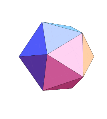
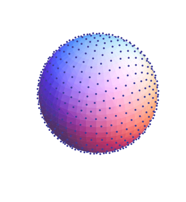
Figure 1: On the left is the $s=1$ icosahedral approximation to the sphere and on the right the $s=8$ equilateral triangle refinement of the icosahedron , illustrated by projecting each vertex at fixed angles from the center of the icosahedron to the unit sphere.

To approach the Wilson-Fisher conformal field theory in the continuum limit, we need to tune $\beta$ to the critical point. The relative scale between the longitudinal and transverse lattice (“speed of light” ) is fixed by the integer spacing of descendants of the primary operators. There are no other free parameters. For example the leading primary operator odd under $Z_{2}$ has a sequence of descendants $\Delta_{l}=1/2+\eta/2+l$ for $l=0,1,...$. The first 3 states were clearly identified with modest calculations, verifying the integer spacing and determining the anomalous contribution $\eta$.

3 Numerical Results

The number of sites on one icosahedral shell is $2+10s^{2}$. We chose our cylinders to have lengths which scale with the refinement $T\equiv\rho s$. To locate the critical point, we used aspect ratios $\rho=4,8$ while for computation of the magnetization correlation functions we used only $\rho=8$.

The critical point $\beta_{c}$ was determined first by constructing a sequence of pseudo-critical $\beta$-values defined as matching points of the Binder cumulants[3],

$$U(\beta,s,\rho)=1-\frac{\langle M^{4}\rangle}{3\langle M^{2}\rangle^{2}}$$ (4)

for $s_{p+1}=rs_{p}$ at consecutive $p$-values. This was done for several values of $r$ in the range $1.5\leq r\leq 5$. We also numerically obtained the subleading terms in the approach to the fixed point predicted by the Renormalization Group. Subsequently we improved the estimate by performing a global fit of the scaling relation,

$$U(\beta,s,\rho)\simeq U(\beta_{c},\infty,\rho)+a_{1}(\rho)[\beta-\beta_{c}]s^{1/\nu}+b_{1}(\rho)s^{-\omega}$$ (5)

to many independent simulations ($\rho=4,8)$, a subset of which appear in Fig. 2, of the scaling relation where the exponents $\nu$ and $\omega$ were held constrained to agree with the published values [4]. We find $\beta_{c}$ = 0.16098698(2), $U(\beta_{c},\infty,4)$ = 0.3040(2) and $U(\beta_{c},\infty,8)$ = 0.1876(2).

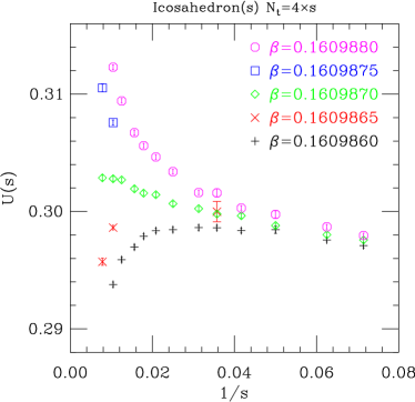
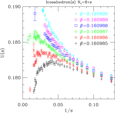
Figure 2: Determining $\beta_{c}$ from the Binder cumulants $U(s)=1-\langle M^{4}\rangle/3\langle M^{2}\rangle^{2}$ near the pseudo-critical point for two different aspect ratios $\rho$ and increasing values of s.

We started our study employing the Swendsen-Wang cluster algorithm [5] but switched to the more efficient single cluster Wolff algorithm [6]. For our final results on the spin-spin correlation function, we generated ensembles at $\beta=0.160987$. Each independent run was thermalized using 2048 sweeps of the Wolff algorithm followed by 8192 sweeps with one estimate of the spin-spin correlation function after each sweep. We defined a sweep to be $19s/2$ Wolff cluster updates which leads to the average number of spins flipped each sweep equal to the total volume. All results for a given run are then averaged together to form a single blocked estimate and many thousands of independent block estimates are combined to form the ensemble at each $s$. The jackknife method was used to estimate errors.

We projected the spin-spin correlations function on spherical harmonics,

$$C_{l}(t)=\sum_{m,t_{0},x,y}Y_{lm}(\Omega_{x})\;\langle\sigma(t+t_{0},x)\sigma(t_{0},y)\rangle\;Y_{lm}(\Omega_{y})$$ (6)

where $Y_{lm}(\Omega_{x})$ is spherical harmonic evaluated at the angular position of the site $x$, weighted by 1/3 of the area of the adjacent spherical triangle projected on the unit sphere as illustrated in Fig. 1. This represents a finite element approach giving an improved approximation to orthonormality of the discrete spherical harmonic. As we are only interested in the rotationally-invariant part of the correlation function on any given lattice, we have summed over the azimuthal quantum number, $m$.

In addition we found it very useful to evaluate the spin-spin correlation function using the momentum space single cluster improved estimator method [7]. The connected correlator for the lowest mass discrete eigenstate of transfer matrix on our periodic lattice is exactly represented by a single hyperbolic cosine,

$$C_{l}(t)=A_{l}\cosh(-\mu_{l}(t-T/2))\;,$$ (7)

at discrete values $t=0,\cdots,T-1$. We transform this to momentum space,

$$\widetilde{C}_{l}(k)=\frac{1}{T}\sum_{t=0}^{T-1}e^{\textstyle itk}\;C_{l}(t)=c_{0}\delta_{l,0}\delta_{k,0}+a_{l}\frac{(1-e^{-\mu_{l}T})\sinh(\mu_{l})}{\sinh^{2}(\mu_{l}/2)+\sin^{2}(k/2)}.$$ (8)

where $k=2\pi q/T$ with $q=0,\cdots,T-1$ is the momentum conjugate to $t\equiv\log r$ along the cylinder. Since our value of $\beta\simeq\beta_{c}$ is slightly larger that the pseudo-critical coupling at any finite $s$, we expect that our $l=0$ correlation function will have a small disconnected contribution. This contributes a non-analytic term, $c_{0}\delta_{k,0}$. In momentum space the disconnected piece can in principle be isolated by subtracting a smooth extrapolation of $C_{0}(k)$ from $k\neq 0$ to $k=0$.

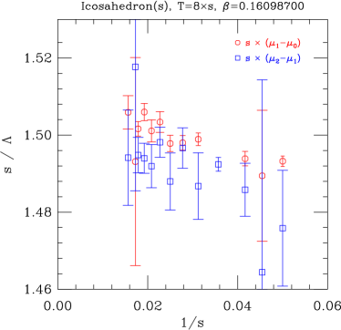
Figure 3: The left figure shows the scaling of $\Lambda$ relative to $s$. The extrapolated value is roughly 1.51(1) with the uncertainty dominated by the systematic difference between the two estimates. The right figure tests the hypothesis of integer level spacing between primaries and descendents by comparing the level spacing between the first and second descendents to the spacing between the primary and its first descendent. We fit to a linear function and find an intercept of 0.994(4) and slope of 0.0(2) with $\chi^{2}/\mbox{dof}=0.43$ for 11 dof.

We found that our data require parameterizing the ground state plus at least three higher mass states to get excellent fits with $\chi^{2}/\mbox{dof}\lesssim 1$ and estimates of ground state masses which are essentially free of higher state contamination. These represent possible high states either propagating forward in the $Z_{2}$ even or propagation backward in $Z_{2}$ odd sectors. While the dimension of the higher state coming from the $Z_{2}$ even sector might be lower, its mixing will also be proportional to the 3 point coupling of the energy operator and two spin operators. Indeed with higher statistics, we believe quantitative determination of the higher spectrum is well within reach of this method.

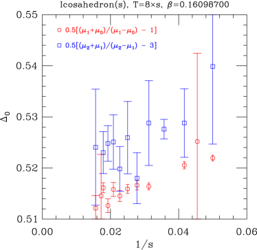
Figure 4: The scaling exponent of lowest $Z_{2}$-odd primary operator vs. $1/s$. The lower (red) points using the primary and first descendant have disconnected contributions that have not been fully determined. A linear extrapolation from upper (blue) points, using the first two descendants which have no disconnected contributions, gives $\Delta_{0}=0.517(5)$, is consistent with the best published estimate 0.5182(3) [4].

Once we have determined the $\mu_{l}$’s, we relate them to the eigenvalues of the dilatation operator up to a single unknown constant: $\mu_{l}=\Lambda^{-1}[\Delta_{0}+l]$ where $\Lambda^{-1}\simeq c_{1}/s$ as $s\to\infty$. Numerically, we find $c_{1}\approx 1.51(1)$ with the uncertainty dominated by systematic error. Clearly, we see evidence for sub-leading contributions $\mathcal{O}(1/s^{2})$ as well in the left figure of Fig. 3. We then test for the equal spacing rule of descendants by examining the ratios, $(\mu_{l+2}-\mu_{l+1})/(\mu_{l+1}-\mu_{l})$, as shown on the right in Fig. 3. Using this confirmation, we are able to estimate numerically the scaling dimension of the primary operator using ratios,

$$\Delta_{0}=\frac{l-l^{\prime}}{2}\left[\frac{\mu_{l}+\mu_{l^{\prime}}}{\mu_{l}-\mu_{l^{\prime}}}-\frac{l+l^{\prime}}{l-l^{\prime}}\right]$$ (9)

as shown in Fig. 4.

We end up with what we feel is a quite conservative estimate of $\eta=0.034(10)$, consistent with other estimates [4]. Moreover this method can be extended to include additional primary operators in both the $Z_{2}$-odd and $Z_{2}$-even sectors as well as direct test of the restoration of full conformal symmetry for 2- and 3-point correlators.

4 Discussion

We have presented a simple example of lattice radial quantization for the 3D Ising model. This raises important questions and suggests further applications.

For the 3D Ising radial quantization, we have chosen a simple approximation to the sphere by a triangular refinement of the icosahedron with “flat” sides. This is reflected in the action by assigning equal weights on all the nearest neighbor links. Viewed in the language of Regge calculus, this geometry has all the curvature concentrated at 12 exceptional vertices of the underlying icosahedron that are bounded by 5 rather than 6 triangles. We are implicitly making the conjecture that by virtue of maintaining exact icosahedral symmetry the continuum limit gives back the symmetry of $\mathbb{S}^{2}$, indeed the full conformal group. Our modest numerical results to date support this conjecture, but we are undertaking more stringent numerical test on the spectrum and correlators. It is an open question whether the conical singularities at the vertices of the icosahedron are irrelevant to the continuum spectrum. If necessary one might introduce improved triangulation of the metric on $\mathbb{S}^{2}$, similar to our improvement of the $Y_{lm}$ weights in our correlation measurement. On the other hand, it is also interesting to ask if the simpler geometry of a refined cube is adequate, since applications to 4D gauge theories are probably easier to formulate on concentric 3D hypercubes.

The next simplest model beyond the 3D Ising model to consider is the 3D O(N) model, which because of the analytical results in the large N limit is an excellent test-bed for the method. We are considering generalization to include gauge fields and fermions in 3D and 4D. Each of these steps will require careful consideration to make sure that there are no obstructions to taking the continuum limit. There maybe subtle issues for example with fermions on a spherical manifolds and potentially relevant conformal symmetry breaking operators the don’t vanish in the continuum. Even more challenging are theories that are not quite conformal where the dilatation operator is no longer a conserved quantity, such as those exhibiting asymptotic freedom in the UV and softly broken conformality near an IR fixed point.

References

- [1] S. Fubini, A. J. Hanson and R. Jackiw, “New approach to field theory,” Phys. Rev. D 7, 1732 (1973).
- [2] J. L. Cardy, “Universal amplitudes in finite-size scaling: generalization to arbitrary dimensionality,” J. Phys. A 18, L757 (1985).
- [3] K. Binder, “Finite size scaling analysis of Ising model block distribution functions,” Z. Phys. B 43, 119 (1981).
- [4] A. Pelissetto and E. Vicari, “Critical phenomena and renormalization group theory,” Phys. Rept. 368, 549 (2002) [cond-mat/0012164].
- [5] R. H. Swendsen and J. -S. Wang, ”Nonuniversal critical dynamics in Monte Carlo simulations,” Phys. Rev. Lett. 58, 86 (1987).
- [6] U. Wolff, “Collective Monte Carlo Updating for Spin Systems,” Phys. Rev. Lett. 62, 361 (1989).
- [7] C. Ruge, P. Zhu and F. Wagner, “Correlation function in Ising models,” Physica A 209, 431 (1994) [hep-lat/9403009].