Electricity Cost Minimization for a Residential Smart Grid with Distributed Generation and Bidirectional Power Transactions

Abstract

In this paper, we consider the electricity cost minimization problem in a residential network where each community is equipped with a distributed power generation source and every household in the community has a set of essential and shiftable power demands. We allow bi-directional power transactions and assume a two-tier pricing model for the buying and selling of electricity from the grid. In this situation, in order to reduce the cost of electricity we are required to make, 1) Scheduling decisions for the shiftable demands, 2) The decisions on the amount of energy purchased from the gird by the users, 3) The decisions on the amount of energy sold to the grid by the users. We formulate a global centralized optimization problem and obtain the optimal amount of electricity consumed, sold and purchased for each household, respectively by assuming the availability of all current and future values of time-varying parameters. In reality, the lack of perfect information hampers the implementation of such global centralized optimization. Hence, we propose a distributed online algorithm which only requires the current values of the time-varying supply and demand processes. We then compare and determine the tradeoff between both formulations. Simulation results show that the proposed schemes can provide effective management for household electricity usage.

I Introduction

While the traditional electricity grid has maintained its current state for many decades, there is a growing need to transit to a newer state with increasing demands from renewable energy integration and reducing dependency on fossil fuel. National governments and relevant industries have been making significant efforts in the development of future electrical grids or smart grids. A smart grid [1]-[3] is known as an intelligent electricity network that uses two-way flows of electricity and information to create an automated and distributed power delivery system which can help save energy, reduce costs, increase reliability and transparency.

There are two significant advantages of the smart grid: improved integration for renewable energy (e.g. wind, solar energy) and increased capability for demand-side management. In residential households, the electricity generated from renewable distributed plants such as solar panels can help the consumer save on electricity costs and in systems supporting sell back policies like net metering, residents can even turn a profit by selling the extra renewable energy back to the power grid [4]. While typical renewable energy sources offer a cheaper and cleaner energy supply, they introduce supply uncertainty due to the volatility of their generation [5]. It is therefore important to include a complementary technology [6], or provide a mixture of traditional power to mitigate or cancel the volatility [7] [8].

Another way to mitigate this problem is to manage this supply variability with demand side flexibility [9] [10]. In [9], the authors suggested that consumers who could tolerate serving delays within a pre-agreed deadline can be offered electricity at a lower price by renewable power suppliers. This essentially allows a lower price of renewable energy to consumers willing to provide this extra time flexibility. The renewable power supplier can now use this flexibility to deliver the energy when it is available. Based on this model, the authors in [10] investigated the problem of allocating energy from renewable sources to flexible consumers in electricity markets. The renewable plant must serve consumers within a specified delay window, and incurs a cost of drawing energy from other (possibly non-renewable) sources if its own supply is not sufficient to meet the deadline. An natural extension to this work involving consumer flexibility is the consideration of a distributed renewable energy source that allows consumers to not only consume power from the grid but sell it back too.

In this paper, we consider the electricity cost minimization problem with a renewable based Distributed Generation (DG) and bidirectional power transactions in a residential smart grid. Each household is equipped with a mixed renewable power source which consists of both wind and solar generators. There are two types of appliances in each home: essential and shiftable appliances, which leads to essential and shiftable power demands in the entire residential system. We allow bi-directional power transactions and assume a dynamic pricing model for the buying and selling of electricity from the grid. In order to reduce the cost of electricity we are required to make, 1) Scheduling decisions for the shiftable demands, 2) The decisions on the amount of energy purchased from the grid by the users, 3) The decisions on the amount of energy sold to the grid by the users.

We first formulate a global optimization problem and obtain the optimal amount of electricity consumed, sold and purchased for each household, by assuming the availability of all current and future values of time-varying parameters. Consequently, we propose a distributed online algorithm which only requires the current values of the time-varying supply and demand processes. A comparison of the simulation results show that the proposed schemes can provide effective management for household electricity usage.

The rest of the paper is organized as follows. In Section II, the system models are introduced. The formulation for the global optimization problem with perfect information is proposed in Section III. The distributed online algorithm with Lyapunov optimization is presented in Section IV. Section V presents the simulation results of the proposed schemes. Finally, we conclude the paper in Section VI.

II System Model

II-A Mixed Distributed Renewable Energy Source

In this subsection, we present the models for the distributed energy sources modelled as a combination of both a photovoltaic (PV) module and a wind turbine, modelled separately^∗.

II-A1 Output Power of a PV Module

The irradiance data for a particular day in each season can be described as a bimodal distribution function. The data are divided into two groups, each is described using a unimodal distribution function, and a Beta pdf is utilized as [5]:

$$f_{b}(s)=\left\{\begin{array}[]{l}\frac{\Gamma(\alpha+\beta)}{\Gamma(\alpha)\Gamma(\beta)}\ast s^{(\alpha+1)}\ast(1-s)^{(\beta-1)}\\ 0\quad otherwise\end{array}\right.$$ (1)

where $s$ is the solar irradiance ($kW/m^{2}$), $f_{b}(s)$ is the Beta distribution function of $s$ and $\alpha$, $\beta$ are the parameters of the Beta distribution function.

The output power of the PV module is dependent on the solar irradiance and ambient temperature of the site as well as the characteristics of the module itself. Therefore, once the Beta pdf per sitel is generated for a specific time segment, the output power during the different states is calculated for this segment using the following:

$$\begin{array}[]{l}T_{c_{y}}=T_{A}+s_{ay}\left(\frac{N_{OT}-20}{0.8}\right)\\ FF=\frac{V_{MPP}*I_{MPP}}{V_{oc}*I_{sc}}\\ I_{y}=s_{ay}\left[I_{sc}+K_{i}(T_{c_{y}}-25)\right]\\ V_{y}=V_{oc}-K_{v}*T_{c_{y}}\\ P_{s_{y}}(s_{ay})=N*FF*V_{y}*T_{y}\end{array}$$ (2)

where $T_{c_{y}}$ is the cell temperature ${}^{\circ}\mathrm{C}$ during state $y$, $T_{A}$ is the ambient temperature ${}^{\circ}\mathrm{C}$, $K_{v}$ is the voltage temperature coefficient V$/^{\circ}\mathrm{C}$; $K_{i}$ is the current temperature coefficient A$/^{\circ}\mathrm{C}$; $N_{OT}$ is the nominal operating temperature of cell in ${}^{\circ}\mathrm{C}$; $FF$ is the fill factor; $I_{sc}$ is the short circuit current in A; $V_{oc}$ is the open-circuit voltage in V; $I_{MPP}$ is the current at maximum power point in A; $V_{MPP}$ is the voltage at maximum power point in V; $P_{s_{y}}$ is the output power of the PV module during state $y$; $s_{ay}$ is the average solar irradiance of state $y$.

II-A2 Output Power of a Wind Turbine

The wind speed profile is used to generate a corresponding output power for use in the distributed power generation. Rayleigh pdf is used to represent the wind speed profile for each time segment, given as:

$$f_{r}(v)=\left(\frac{2v}{c^{2}}\right)\exp\left[-\left(\frac{v}{c}\right)^{2}\right]$$ (3)

where $c=1.128v_{m}$.

The output power of a wind turbine is dependent on the wind speed at the site as well as the parameters of its power performance curve. Therefore, once the Rayleigh pdf is generated for a specific time segment, the output power during the different states is calculated for this segment as [5]:

$$P_{Vw}(v_{aw})=\left\{\begin{split}&0&0\leq v_{aw}\leq v_{ci}\\ &P_{rated}*\frac{v_{aw}-v_{ci}}{v_{r}-v_{ci}}&v_{ci}\leq v_{aw}\leq v_{r}\\ &P_{rated}&v_{r}\leq v_{aw}\leq v_{co}\\ &0&v_{co}\leq v_{aw}\end{split}\right.$$ (4)

where $v_{ci}$, $v_{r}$ and $v_{co}$ are cut in speed, rated speed, and cut-off speed of the wind turbine, respectively, $P_{Vw}(v_{aw})$ is output power of the wind turbine during state $w$, $v_{aw}$ is average wind speed of state.

To incorporate the output power of the solar PV DG and wind turbine DG units as multistate variables in the global formulation, the continuous pdf of each has been divided into states (periods), in each of which the solar irradiance and wind speed are within specific limits. In other words, for each time segment, there are a number of states for the solar irradiance and wind speed. The probability of the solar irradiance and wind speed generation for each state during any specific hour is calculated as follows:

$$\Omega_{s}(G_{y})=\int_{s_{y1}}^{s_{y2}}f_{b}(s)ds,$$ (5)

$$\Omega_{v}(G_{w})=\int_{v_{w1}}^{v_{w2}}f_{w}(v)dv$$ (6)

where $\Omega_{s}(G_{y})$ is the probability of the solar irradiance being in state $y$; $\Omega_{v}(G_{w})$ probability of wind speed being in state $w$; $s_{y1}$ and $s_{y2}$ are the solar irradiance limits of state $y$; $v_{w1}$ and $v_{w2}$ are the wind speed limits of state $w$.

Assuming that wind speed states and solar irradiance states are independent, the probability of any combination of them ($\Omega\{C_{g}\}$) is obtained by convolving the two probabilities:

$$\Omega\{C_{g}\}=\Omega_{s}(G_{y})\ast\Omega_{v}(G_{w}).$$ (7)

We define a supply function $S(t)$ to indicate the energy generated by the renewable sources at time $t$, and obtain

$$S(t)=\sum_{g=1}^{G}P_{g,t}\Omega\{C_{g}\}$$ (8)

where $P_{g,t}$ is the mixed power of the $g$ state at time $t$. We have a maximum limit on the electricity that can be generated by the renewable plant i.e. $0\leq S(t)\leq S_{max},\forall t.$

II-B Residential Smart Grid Model

Let $\mathcal{N}$ denote the set of users in a residential network, where the number of users, each representing one household is $N\triangleq\mid\mathcal{N}\mid$. We consider the residential smart grid in which the electricity from the power grid and renewable sources are shared by these $N$ users (homes), each one of which is equipped by a smart meter. The smart meter connects with all the household appliances and not only manages the electricity flow, but also schedules the power consumption of each appliance in terms of the collected user's preference information. Based on all the collected information, a centralized scheduler will globally optimize the hourly power consumption and schedule all appliances.

The appliances that define a household are divided into two types: essential and shiftable appliances. Essential appliances are defined as appliances that have a fixed energy requirement that would not be subjected to scheduling decisions. These appliances include television sets and refrigerators. The optimization process would ensure a continuous supply of electricity for these. Shiftable appliances allow the smart meter to schedule electricity loads to minimize electricity cost. These appliances could include dishwashers, washing machines and clothes dryers. We denote the total essential and shiftable load for the $n$th user at time $t$ as $a_{n,e}(t)$ and $a_{n,s}(t)$, respectively. Then, the total essential and shiftable load across all users at time $t$ can be respectively calculated as

$$A_{e}(t)=\sum_{n\in\mathcal{N}}a_{n,e}(t),\quad A_{s}(t)=\sum_{n\in\mathcal{N}}a_{n,s}(t).$$

II-C Delay-Aware Power Transactions

In our model, the energy produced by the distributed energy source at time $t$ can either be used to serve essential demand, shiftable demand or can be sold to the grid. Let $S_{e}(t)$ and $S_{s}(t)$ denote the electricity taken from the renewable plant to satisfy the essential and shiftable demand at time $t$, respectively. Let $S_{p}(t)$ denote the electricity that is sold by the customer to the grid at time $t$. Then, we have

$$S_{e}(t)+S_{s}(t)+S_{p}(t)=S(t),\quad\forall t.$$

However, the renewable energy may not be enough to meet all of the requests within a timely manner, and hence we also decide to purchase an amount of electricity from the power grid. Let $G(t)$, $G_{e}(t)$ and $G_{s}(t)$ denote respectively the total electricity purchased from the grid, the portion of electricity taken from grid to serve essential and shiftable loads at time $t$, we have,

$$G(t)=G_{e}(t)+G_{s}(t),\quad\forall t.$$

Meanwhile, in order to formulate the problem mathematically, we put a limit on max power that can be purchased from the grid, i.e. $0\leq G(t)\leq G_{max},\forall t.$

Let $p(t)$ denote the cost of electricity taken from the grid at time $t$. Let $\gamma(t)$ denote the price set by the grid to purchase electricity at time $t$. The instantaneous cost of electricity at time $t$, denoted by $C(t)$, is then given by,

$$\begin{split}C(t)&=p(t)G(t)-\gamma(t)S_{p}(t)\\ &=p(t)[G_{e}(t)+G_{s}(t)]-\gamma(t)[S(t)-S_{e}(t)-S_{s}(t)].\end{split}$$ (9)

We assume that shiftable loads are flexible, and can tolerate their demands being satisfied with some delay. We store all the shiftable demands in a queue. The electricity demands in this queue are served in a FIFO manner and the queue is then updated according to:

$$Q(t+1)=\max\bigg{\{}Q(t)-G_{s}(t)-S_{s}(t),0\bigg{\}}+A_{s}(t).$$

Let $\bar{Q}$ denote the expected time average of the demand queue,

$$\bar{Q}=\text{lim}_{T\rightarrow\infty}\>\frac{1}{T}\sum_{t=0}^{T-1}E\bigg{\{}Q(t)\bigg{\}}<Q_{max}.$$

The demands are served with finite delays if $Q_{max}<\infty$.

III Problem Formulation

Our objective now is to minimize the expected time average cost of electricity subject to satisfying the essential demands and guaranteeing the shiftable demands with a worst case delay bound $D_{max}$. The optimization problem can now be formulated as follows,

$$P_{1}=\min_{G_{e}(t),G_{s}(t),S_{e}(t),S_{s}(t)}\>\text{lim}_{T\rightarrow\infty}\>\frac{1}{T}\sum_{t=0}^{T-1}E\left\{C(t)\right\}$$ (10)

subject to,

$$G_{e}(t)+S_{e}(t)=A_{e}(t),\quad\forall t,$$ (11)

$$0\leq S(t)\leq S_{max},\quad\forall t,$$ (12)

$$0\leq G(t)\leq G_{max},\quad\forall t,$$ (13)

$$Q(t+1)=\max\bigg{\{}Q(t)-G_{s}(t)-S_{s}(t),0\bigg{\}}+A_{s}(t),$$ (14)

$$\bar{Q}<Q_{max}$$ (15)

where $C(t)$ is given by (9). The backward dynamic programming approach can be used to solve problem (10) subject to the constraint set (11)-(15). The state vector is given by $x_{t}=(S_{t},A_{e,t},A_{s,t},p_{t},\gamma_{t})$, where $S_{t}$ is the renewable supply, $A_{e,t}$ and $A_{s,t}$ are the essential and shiftable demand respectively, and $p_{t}$, $\gamma_{t}$ are the market price for buying and selling electricity respectively. Our control is assumed as $u_{t}=(G_{e,t},G_{s,t},S_{e,t},S_{s,t})$, the backward dynamic programming algorithm is given by the following equation [9]:

$$J_{t}(x)=\min_{u_{t}\in U_{t}(x)}\left\{C(x,u_{t})+\sum_{y\in Y_{t+1}}J_{t+1}(y)\right\}$$

where $J_{t}(x)$ is the value function of period $t$, $C(x,u_{t})=p_{t}(G_{e,t}+G_{s,t})-\gamma_{t}(S_{t}-S_{e,t}-S_{s,t})$ is the electricity cost incurred at each period, $U_{t}(x)$ is the feasible region of actions for period $t$, and $Y_{t}$ is the feasible region of the state vector at period $t$.

Since the dynamic programming need global information to solve the problem which may have the disadvantage to capture the time-varying characteristics of the demand and supply in renewable related residential networks. It stands to reason that an algorithm that can make optimal decision without the knowledge of future information should be designed. Inspired by [10], we design a distributed online algorithm which will utilize a Lyapunov optimization technique to solve the optimization problem in a distributed way without a-priori statistical knowledge.

IV Distributed Online Algorithm

IV-A Lyapunov Optimization

Let $P_{1}^{*}$ denote the infimum time average cost of the above problem. The requirement of $\bar{Q}<\infty$ in the above problem does not guarantee a delay bound $D_{max}$. To ensure this bound a delay aware virtual queue is developed. This delay aware virtual queue has the same service rate as that of the actual queue but it grows if the demand is not serviced at time $t$. The virtual queue update equation is,

$$Z(t+1)=\max\bigg{\{}Z(t)-G_{s}(t)-S_{s}(t)+\epsilon 1_{\big{\{}Q(t)>0\big{\}}},0\bigg{\}}$$ (16)

where, $1_{\big{\{}Q(t)>0\big{\}}}$ is an indicator function. The value of this function is 1 if $Q(t)>0$ and 0 otherwise. Thus the delay aware queue grows by an amount $\epsilon$ each time it is not serviced. With the introduction of delay aware virtual queue we have the following Lemma [9].

Lemma 1: If $Z(t)\leq Z_{max}$ and $Q(t)\leq Q_{max}$, then all shiftable devices will get scheduled with a worst case delay of $D_{max}$ where,

$$D_{max}=\left\lceil\frac{Z_{max}+Q_{max}}{\epsilon}\right\rceil.$$

Let $\Theta(t)=(Z(t),Q(t))$ denote the concatenated vector of virtual and real queues. We then define the following Lyapunov function to measure the congestion in the queues,

$$L(\Theta(t))=\frac{1}{2}[Z^{2}(t)+Q^{2}(t)].$$

The conditional 1-slot Lyapunov drift is defined as,

$$\Delta(\Theta(t))=E\bigg{\{}L(\Theta(t+1))-L(\Theta(t))|\Theta(t)\bigg{\}}.$$

Define $V>0$ as a parameter to effect the performance delay tradeoff, we have the following drift plus penalty function, by using the drift plus penalty framework developed in [9],

$$\Delta(\Theta(t))+VE\bigg{\{}C(t)|\Theta(t)\bigg{\}}$$

where $C(t)$ is given by (9). Again using the same techniques in [9] we can show that this function is bounded as,

$$\Delta(\Theta(t))+VE\bigg{\{}C(t)|\Theta(t)\bigg{\}}\leq B+VE\bigg{\{}C(t)|\Theta(t)\bigg{\}}$$

$$+Q(t)E\bigg{\{}\big{(}A_{s}(t)-G_{s}(t)-S_{s}(t)\big{)}|\Theta(t)\bigg{\}}$$

$$+Z(t)E\bigg{\{}\big{(}\epsilon-G_{s}(t)-S_{s}(t)\big{)}|\Theta(t)\bigg{\}}.$$ (17)

Now instead of solving the original problem we minimize this bound on the drift plus penalty function.

IV-B Two-Stage Online Algorithm

In this section, we propose a two-stage online algorithm to minimize the right-hand-side of the drift-plus-penalty bound (17) at every slot $t$ as follows,

1. At each time $t$ observe: $Z(t)$, $Q(t)$, $p(t)$, $\gamma(t)$, $S(t)$, $A_{s}(t)$ and $A_{e}(t)$.
2. Then solve the following optimization problem to obtain the decision variables $\{G_{e}^{*}(t),G_{s}^{*}(t),S_{e}^{*}(t),S_{s}^{*}(t)\}$:

$$\min_{G_{e}(t),G_{s}(t),S_{e}(t),S_{s}(t)}\>VC(t)-\bigg{\{}Q(t)+Z(t)\bigg{\}}\bigg{\{}G_{s}(t)+S_{s}(t)\bigg{\}}$$

subject to constraints (11), (12), (13).
3. Then update the queue equations for next time slot,

$$Q(t+1)=\max\bigg{\{}Q(t)-G_{s}^{*}(t)-S_{s}^{*}(t),0\bigg{\}}+A_{s}(t),$$

$$Z(t+1)=\max\bigg{\{}Z(t)-G_{s}^{*}(t)-S_{s}^{*}(t)+\epsilon 1_{\big{\{}Q(t)>0\big{\}}},0\bigg{\}}.$$

Using this algorithm, the problem is decoupled in time. Also we do not require any information about the future values or the expectations. In addition, we observe that the electricity served for essential loads $G_{s}(t)$ and $S_{e}(t)$ are independent with that for shiftable load in the above formulation. Hence, our problem can be separately solved in two stages. In stage I, we will minimize the cost and only introducing essential load as the input; In stage II, we solve the optimization problem for shiftable load.

IV-B1 Stage I, Optimization for Essential Load

At each time slot the instantaneous optimization problem is,

$$\min_{G_{e}(t),\!G_{s}(t),\!S_{e}(t),\!S_{s}(t)}\>\!\!VC(t)\!-\!\bigg{\{}Q(t)\!+\!Z(t)\bigg{\}}\!\bigg{\{}G_{s}(t)\!+\!S_{s}(t)\!\bigg{\}}$$

subject to constraints (11), (12), (13). Rearranging the terms in the above objective function we get the following optimization problem for the essential load,

$$\min_{G_{e}(t),S_{e}(t)}\>V\bigg{(}p(t)G_{e}(t)+\gamma(t)S_{e}(t)\bigg{)}$$ (18)

subject to,

$$G_{e}(t)+S_{e}(t)=A_{e}(t),\quad\forall t.$$ (19)

Replace $G_{e}(t)=A_{e}(t)-S_{e}(t)$ in the above objective function, we get the following unconstrained optimization problem in only one variable,

$$\min_{S_{e}(t)}\>V(\gamma(t)-p(t))S_{e}(t).$$ (20)

From this equation it is obvious that for cost minimization we should adopt the following strategy,

$$G_{e}^{*}(t)=\Bigg{\{}\begin{array}[]{c}\tilde{G}=\min\big{(}G_{max},A_{e}(t)\big{)},\quad\text{if}\>p(t)<\gamma(t)\\ \max\big{(}A_{e}(t)-\tilde{S},0\big{)},\quad\text{if}\>p(t)\geq\gamma(t).\end{array}$$ (23)

$$S_{e}^{*}(t)=\Bigg{\{}\begin{array}[]{c}\tilde{S}=\min\big{(}S(t),A_{e}(t)\big{)},\quad\text{if}\>\gamma(t)\leq p(t)\\ \max\big{(}A_{e}(t)-\tilde{G},0\big{)},\quad\text{if}\>\gamma(t)>p(t).\end{array}$$ (26)

This result is very simple and it says that we should use maximum power from the grid if the price of purchasing electricity is less than price of selling renewable electricity back to the grid. Otherwise utilize maximum power from the renewable source to satisfy the essential load demands. We assume that there is always enough power available to serve the essential demands in any time slot.

IV-B2 Stage II, Optimization for Shiftable Load

Once the decision on $G_{e}^{*}(t)$ and $S_{e}^{*}(t)$ for essential load are obtained we have to decide about the remaining renewable and grid power. The power that is available for shiftable demands is,

$$\tilde{S}_{max}=\max(S(t)-S_{e}^{*}(t),0),$$ (27)

$$\tilde{G}_{max}=\max(G_{max}-G_{e}^{*}(t),0).$$ (28)

The objective function for the shiftable problem now contains the remaining terms and the remaining constraints. After some re-arrangement of terms in the objective function the instantaneous optimization problem to obtain variables $G_{s}(t)$ and $S_{s}(t)$ is now as follows,

$$\min_{G_{s}(t),S_{s}(t)}\>\bigg{\{}G_{s}(t)\bigg{(}Vp(t)-(Q(t)+Z(t))\bigg{)}\bigg{\}}+$$

$$\bigg{\{}S_{s}(t)\bigg{(}V\gamma(t)-(Q(t)+Z(t))\bigg{)}\bigg{\}}$$ (29)

subject to constraints (27), (28). We can then decide the optimum variables based on appropriate threshold type policy.

IV-C Real-Time Distributed Decision

There are four possible cases depending on the current prices and queue states.

IV-C1 Case I: $Vp(t)>Q(t)+Z(t)$ and $V\gamma(t)>Q(t)+Z(t)$

This situation indicates any or all of the following:

• the queue lengths are small

• for given $V$, $p(t)$ is large i.e. price of buying electricity from grid is high

• for given $V$, $\gamma(t)$ is large i.e. price of selling electricity to grid is high

In this situation (also evident from the objective function), shiftable load should not be scheduled and instead we should sell all the electricity to the grid i.e.

$$G_{s}^{*}(t)=0,\quad S_{s}^{*}(t)=0,\quad S_{p}^{*}(t)=\tilde{S}_{max}.$$

IV-C2 Case II: $Vp(t)>Q(t)+Z(t)$ and $V\gamma(t)<Q(t)+Z(t)$

This situation is possible when $p(t)\geq\gamma(t)$. In this case, we should serve the shiftable queue using renewable energy only. The shiftable queue should not be served from the grid and any remaining renewable energy left after servicing the shiftable queue should be sold to the grid.

$$G_{s}^{*}(t)=0,$$

$$S_{s}^{*}(t)=\min(\tilde{S}_{max},Q(t)),$$

$$S_{p}^{*}(t)=\max(\tilde{S}_{max}-S_{s}^{*}(t),0).$$

IV-C3 Case III: $Vp(t)<Q(t)+Z(t)$ and $V\gamma(t)>Q(t)+Z(t)$

This situation is possible when $p(t)<\gamma(t)$. This case results in a situation where the customer would sell all the renewable electricity to the grid and purchase electricity from the grid to serve the shiftable demands in the queue. However, to prevent users to buy energy from the grid and sell it back, a rational pricing model will make sure that $p(t)$ will never less than $\gamma(t)$. Hence, this case will not happen.

IV-C4 Case IV: $Vp(t)<Q(t)+Z(t)$ and $V\gamma(t)<Q(t)+Z(t)$

This situation means any or all of the following:

• queue thresholds are high

• price of electricity from grid is low

• price offered by grid for renewable energy is also low

In this case we should serve the queue using the energy from the grid as well as the renewable source. For this situation we have two further sub-cases:
Sub-case I (if $p(t)\geq\gamma(t)$): in this case, the consumers use maximum energy from the renewable source to serve shiftable loads. The remaining demands in the queue should then be served using grid energy. If some renewable energy remains after servicing the queue then it should be sold to the grid.

$$S_{s}^{*}(t)=\min(\tilde{S}_{max},Q(t)),$$

$$G_{s}^{*}(t)=\min(Q(t)-S_{s}^{*}(t),\tilde{G}_{max}),$$

$$S_{p}^{*}(t)=\max(\tilde{S}_{max}-S_{s}^{*}(t),0).$$

Sub-case II (if $p(t)<\gamma(t)$): Based on the same reason expressed in Case III, this case also will not happen.

V The Simulation Analysis

We consider 10 customers (homes) and each customer is selected to have 20 essential appliances and 20 shiftable appliances. We have a set up similar to [11], where the essential appliances may include electric stoves (daily usage $E$: 1.89 kWh for self-cleaning and 2.01 kWh for regular), lighting (daily usage for 10 standard bulbs: 1.00 kWh). Based on this set up, the essential load $A_{e}(t)$ for each hour can be obtained. The shiftable appliances may include dishwashers (daily usage $E$: 1.44 kWh), washing machines (daily usage $E$: 1.49 kWh for energy-start, 1.94 kWh for regular) and clothes dryers (daily usage $E$: 2.50 kWh). To describe the time-varying characteristic of the shiftable load, we model the shiftable demand $A_{s}(t)$ as i.i.d. over slots and uniformly distributed over the integers $\{0,1,\cdots,A_{s,max}\}$. We assume that market prices for purchasing electricity from the grid is $p(t)=0.3$ cents at daytime hours, i.e., from 8:00 in the morning to 12:00 at night and $p(t)=0.1$ cents during the night, i.e., from 12:00 at night to 8:00 AM the day after. Meanwhile, the selling price is set at $\gamma(t)=0.2$ cents during daytime hours and $\gamma(t)=0.1$ cents during the night.

V-A Electricity Cost

We compare the proposed bidirectional transaction scheme with dynamic programming (BTS-DP) and Lyapunov optimization (BTS-LO) against a simple ``Purchasing Only Strategy (POS)'' which tries to use all the available renewable resource $S(t)$ and only buy from the market as a last resort if the produced renewable energy cannot satisfy the current essential and shiftable load. Fig. 1 shows the cumulative electricity costs in different power transaction schemes. It is shown that the energy costs achieved by the proposed bidirectional transaction schemes are less than that in the POS. This is because the proposed schemes are not only able to sell the produced renewable energy to the grid to obtain financial credits, but also schedule the shiftable loads to the lower electricity price periods to reduce electricity consumption costs. We note that the total electricity cost in the BTS-LO case is higher than that in the BTS-DP. That is, the BTS-LO is a distributed online optimization and requires less information than BTS-DP. However, we can obtain the different costs in BTS-LO by adjusting the parameters $V$ and $\epsilon$, which is related to the delay suffered by shiftable load.

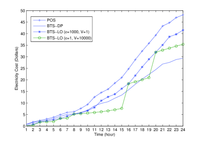
Figure 1: Electricity cost in terms of different power transaction schemes.

V-B Delay

To illustrate the delay in the proposed scheme, we use $log_{10}$ (Actual Demand Queue ($Q$)) to compare the delay between BTS-DP with infinite delay constraint and BTS-LO with delay constraint ($D_{max}$). The delay in terms of different scenarios have shown in Fig. 2. In Fig. 2, it is note that the $log_{10}$ (Actual Demand Queue ($Q$)) has the highest value in the dynamic programming solution, as it achieves the lowest energy cost. In addition, selecting different parameters $V$ and $\epsilon$ in real-time algoirthm BTS-LO, we can adjust the delay and achieve corresponding electricity costs (as shown in Fig. 1), and thus, achieve various tradeoff of the consumers' electricity usage preference: power consumption vs delay tolerance.

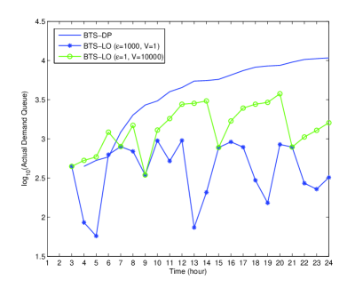
Figure 2: Delay comparison between the bidirectional transaction scheme with dynamic programming and Lyapunov optimization.

VI Conclusion

In this paper, we presented a bidirectional power transaction mechanism to minimize the electricity cost in the residential smart grid. According to the endurance of the serving delay, the residential load is classified into two types: essential load and shiftable load. In order to satisfy both of the loads, consumers can purchase the power from grid or use the produced renewable power. Since the consumers also can sell the produced renewable power to grid for benefit, the shiftable load can be stacked in a queue, given that it will be served within a pre-agreed deadline. To decide the amount of electricity consumed, sold and purchased, we then formulate a global centralized optimization problem and provide a distributed online algorithm by using Lyapunov optimization solution. Simulations confirms that our proposed mechanism is able to balance the tradeoff between the power consumption and the allowable delay in the residential networks. Meanwhile, the effectiveness of distributed online algorithms with limited information is compared with the bound provided by the centralized off-line algorithm with global information.

VII Acknowledgment

This research is partly supported by SUTD-ZJU/RES/02/2011, International Design Center, EIRP, and SSE-LUMS via faculty research startup grant.

References

- [1] S. M. Amin and B. F. Wollenberg, ``Toward a smart grid: Power delivery for the 21st century,'' IEEE Power Energy Magzine, vol. 3, no. 5, pp. 34-41, September/October 2005.
- [2] The Smart Grid: An Introduction. The US Department of Energy, 2008.
- [3] P. Zhang, F. Li and N. Bhatt, ``Next-Generation Monitoring, Analysis, and Control for the Future Smart Control Center,'' IEEE Transactions on Smart Grid, vol. 1, no. 2, pp. 186-192, September 2010.
- [4] Toronto Hydro, ``Renewable Energy Standard Offer Program,'' http:// www.torontohydro.com.
- [5] Y. M. Atwa and E. F. EI-Saadany, M. M. A. Salama, and R. Seethapathy,``Optimal Renewable Resources Mix for Distribution Systme Energy Loss Minimization,'' IEEE Transactions on Power System, vol. 25, no. 1, pp. 360-370, February 2010.
- [6] S. Huang, J. Xiao, J. Pekny, G. Reklaitis, and A Liu, ``Quantifying System-Level Benefits from Distributed Solar and Energy Storage.'' Journal of Energy Engineering, vol. 138, no. 2, pp. 33-42, June, 2012.
- [7] S.-Y. Sun, C.-N. Lu, R.-F. Chang and G.-A. G, ``Distributed Generation Interconnection Planning: A Wind Power Case Study,'' IEEE Transactions on Smart Grid, vol. 2, no. 1, pp. 181-189, September 2011.
- [8] J. Liang, G. K. Venayagamoorthy and R. G. Harley, ``Wide-Area Measurement Based Dynamic Stochastic Optimal Power Flow COntrol for Smart Grid with High Variability and Uncertainty,'' IEEE Transactions on Smart Grid, vol. 3, no. 1, pp. 59-69, September 2012.
- [9] A. Papavasiliou and S. S. Oren, ''Supplying Renewable Energy to Deferrable Loads: Algorithms and Economic Analysis,'' in Proc. IEEE PES General Meeting, Minneapolis, Minnesota, July 25-29 2010.
- [10] M. J. Neely, A. Tehrani, and A. Dimakis, ``Efficient Algorithms for Renewable Energy Allocation to Delay Tolerant Consumers," in Proc. IEEE First Int l Conf. Smart Grid Comm. (SmartGridComm), Oct. 2010.
- [11] A. -H. Mohsenian-Rad and G. Q. Maguire, ``Autonomous Demand-Dide Management Based on Ggame-Theoretic Energy Consumption Scheduling for the Future Smart Grid,'' IEEE Transactions on Smart Grid, vol. 1, no. 3, pp. 320-331, December 2010.