Non-linear Evolution of Rayleigh-Taylor Instability in a Radiation Supported Atmosphere

Abstract

The non-linear regime of Rayleigh-Taylor instability (RTI) in a radiation supported atmosphere, consisting of two uniform fluids with different densities, is studied numerically. We perform simulations using our recently developed numerical algorithm for multi-dimensional radiation hydrodynamics based on a variable Eddington tensor as implemented in Athena, focusing on the regime where scattering opacity greatly exceeds absorption opacity. We find that the radiation field can reduce the growth and mixing rate of RTI, but this reduction is only significant when radiation pressure significantly exceeds gas pressure. Small scale structures are also suppressed in this case. In the non-linear regime, dense fingers sink faster than rarefied bubbles can rise, leading to asymmetric structures about the interface. By comparing the calculations that use a variable Eddington tensor (VET) versus the Eddington approximation, we demonstrate that anisotropy in the radiation field can affect the non-linear development of RTI significantly. We also examine the disruption of a shell of cold gas being accelerated by strong radiation pressure, motivated by models of radiation driven outflows in ultraluminous infrared galaxies. We find that when the growth rate of RTI is smaller than acceleration time scale, the amount of gas that would be pushed away by the radiation field is reduced due to RTI.

1. Introduction

The Rayleigh-Taylor Instability (RTI) occurs when a high density fluid is accelerated by a low density fluid in a gravitational field or net acceleration (e.g. Chandrasekhar, 1961; Sharp, 1984). In an astrophysical context, RTI with or without magnetic field has been studied extensively both numerically (e.g. Jun et al., 1995; Dimonte et al., 2004; Stone & Gardiner, 2007a, b) and experimentally (e.g. Andrews & Spalding, 1990; Dalziel, 1993). In most previous studies, support against gravity was provided by a gradient of the gas pressure or magnetic pressure alone. In this paper, we are interested in the dynamics of the RTI when support against gravity is provided primarily by radiation pressure. This situation is expected, for example, in the inner region of accretion disks around compact object; at the interface of an H II region produced by massive star clusters and the surrounding medium (e.g. Krumholz & Matzner, 2009; Jacquet & Krumholz, 2011) and the dusty tori around luminous Active Galactic Nuclei (AGN) (e.g. Krolik, 2007; Schartmann et al., 2010). In ultraluminous infrared galaxies (ULIRGS), radiation pressure on the dust grains may provide the dominant vertical support against gravity and accelerate the cold (neutral) gas outflows observed in these systems (e.g. Murray et al., 2005; Thompson et al., 2005; Martin, 2005). The structure of radiation dominated bubbles around super-Eddington massive stars also depends on whether RTI develops on the bubble interface (e.g. Krumholz et al., 2009; Kuiper et al., 2012). Radiation RTI, together with Kelvin-Helmholtz instability, may also be important to generate the turbulence in the interstellar medium (ISM) (e.g. McKee & Ostriker, 2007). Thus, understanding the effects of radiation field on linear growth rate and non-linear structures of RTI, as well as assessing the role of radiative RTI in driving turbulence and possibly limiting the effectiveness of radiative support and driving (Kuiper et al., 2011; Krumholz & Thompson, 2012), is an important step to understand those physical systems.

Effects of a radiation field on RTI have been studied analytically in the linear regime with different approximations. In the optically thin limit, radiation flux only provides a background acceleration, and both Mathews & Blumenthal (1977) and Jacquet & Krumholz (2011) conclude that stability depends only on the direction of the effective gravitational acceleration. Krolik (1977) studied the global RTI for an incompressible slab of gas accelerated by radiation pressure. Unstable mode exists if local radiative acceleration correlates positively with total optical depth. Recently, Jacquet & Krumholz (2011) examined the effects of radiation field on the stability of the interface between two fluids in the isothermal and adiabatic limits. In the isothermal limit, the radiation flux only provides an effective background acceleration. In the adiabatic limit, the radiation pressure plays the same role as gas pressure. However, the background state they envisage for the linear analysis (two half infinite constant density planes) cannot precisely be in thermal equilibrium (see section 3) with non-zero absorption opacity. This may affect the growth rate they calculate and the evaluation in the non-linear regime when the timescale for thermal evolution is comparable to or shorter than the growth rate of the RTI.

If there is no density jump in a radiation supported atmosphere without magnetic field, the nature of the stability criterion is not completely settled. With the Eddington approximation, Spiegel & Tao (1999) and Shaviv (2001) find that there are global hydrodynamic unstable modes for a hot atmosphere, even for luminosities moderately below the Eddington limit. However, the instabilities found by Spiegel & Tao (1999) are not present in the Shaviv (2001) analysis. Also, Spiegel & Tao (1999) note that Marzec (1978) arrived at a different conclusion by solving the full transfer equation numerically in a PhD thesis. Turner et al. (2005) found overturning modes in simulations with a fixed temperature at the lower boundary, which are consistent with Shaviv’s Type I modes, although the authors find no evidence for the Type II modes (Shaviv, 2001).

Here we will focus on the traditional case for RTI with a high density fluid on top of a low density fluid separated by an infinite thin interface. In the previous analytical studies, simplifications are necessary to make the problem tractable. For example, radiation pressure is usually assumed to be isotropic, which is not true in general at the interface. In this work, we relax these assumptions by solving the radiation hydrodynamic equations numerically. We study both the linear regime, using an Eddington tensor computed self-consistently from the time-independent radiation transfer equation (i.e., we allow for anisotropic radiation pressure at the interface), and we also follow the RTI into the non-linear regime which is not possible in analytical studies. We note in passing that we have also used our numerical methods to test the stability of a radiation supported atmosphere with a smooth density profile, and find no evidence for instability, in agreement with Turner et al. (2005).

The paper is organized as follows. In section 2, we describe the equations we solve and the numerical code we use. We then consider the problem of RTI with a single, initially static interface between two fluids of different density. We describe the background equilibrium state and initial perturbations in section 3, and summarize our results in section 4. In section 5, we describe simulations of RTI in shells being accelerated by radiation forces. We summarize and conclude in section 6.

2. Equations

We solve the radiation hydrodynamic equations in the mixed frame with radiation source terms given by Lowrie et al. (1999). We assume local thermal equilibrium (LTE) and that the Planck and energy mean absorption opacities are the same. Detailed discussion of the equations we solve can be found in Jiang et al. (2012). With a vertical gravitational acceleration $g$, the equations are

$$\frac{\partial\rho}{\partial t}+{\mbox{\boldmath$\nabla$}}\cdot(\rho{\mbox{\boldmath$v$}}) = 0,$$

$$\frac{\partial(\rho{\mbox{\boldmath$v$}})}{\partial t}+{\mbox{\boldmath$\nabla$}}\cdot({\rho{\mbox{\boldmath$v$}}{\mbox{\boldmath$v$}}+{\sf P}}) = \rho{\mbox{\boldmath$g$}}-{\bf\tilde{S}_{r}}({\mbox{\boldmath$P$}}),\$$

$$\frac{\partial{E}}{\partial t}+{\mbox{\boldmath$\nabla$}}\cdot\left[(E+P){\mbox{\boldmath$v$}}\right] = \rho{\mbox{\boldmath$v$}}\cdot{\mbox{\boldmath$g$}}-c\tilde{S}_{r}(E),$$

$$\frac{\partial E_{r}}{\partial t}+{\mbox{\boldmath$\nabla$}}\cdot{\mbox{\boldmath$F$}}_{r} = c\tilde{S}_{r}(E),$$

$$\frac{1}{c^{2}}\frac{\partial{\mbox{\boldmath$F$}}_{r}}{\partial t}+{\mbox{\boldmath$\nabla$}}\cdot{\sf P}_{r} = {\bf\tilde{S}_{r}}({\mbox{\boldmath$P$}}).$$ (1)

Here, $\rho$ is density, ${\sf P}\equiv P{{\sf\boldmath I}}$ (with ${{\sf\boldmath I}}$ the unit tensor) and $P$ is gas pressure, $\sigma_{a}$ and $\sigma_{s}$ are the absorption and scattering opacities. Total opacity (attenuation coefficient) is $\sigma_{t}=\sigma_{s}+\sigma_{a}$. The total gas energy density is

$$E=E_{g}+\frac{1}{2}\rho v^{2},$$ (2)

where $E_{g}$ is the internal gas energy density. We adopt an equation of state for an ideal gas with adiabatic index $\gamma$, thus $E_{g}=P/(\gamma-1)$ and $T=P/R_{\text{ideal}}\rho$, where $R_{\text{ideal}}$ is the ideal gas constant. The radiation pressure ${\sf P}_{r}$ is related to the radiation energy density $E_{r}$ by the closure relation

$${\sf P}_{r}={\sf\boldmath f}E_{r}.$$ (3)

where ${\sf\boldmath f}$ is the variable Eddington tensor (VET). Radiation flux is ${\mbox{\boldmath$F$}}_{r}$ while $c$ is the speed of light. The gravitational acceleration $g$ is fixed to be a constant value along the $-z$ axis. ${\bf\tilde{S}_{r}}({\mbox{\boldmath$P$}})$ and $\tilde{S}_{r}(E)$ are the radiation momentum and energy source terms.

Following Jiang et al. (2012), we use a dimensionless set of equations and variables in the remainder of this work. We convert the above set of equations to the dimensionless form by choosing fiducial units for velocity, temperature and pressure as $a_{0},\ T_{0}$ and $P_{0}$ respectively. Then units for radiation energy density $E_{r}$ and flux ${\mbox{\boldmath$F$}}_{r}$ are $a_{r}T_{0}^{4}$ and $ca_{r}T_{0}^{4}$. In other words, $a_{r}=1$ in our units. The dimensionless speed of light is $\mathbb{C}\equiv c/a_{0}$. The original dimensional equations can then be written to the following dimensionless form

$$\frac{\partial\rho}{\partial t}+{\mbox{\boldmath$\nabla$}}\cdot(\rho{\mbox{\boldmath$v$}}) = 0,$$

$$\frac{\partial(\rho{\mbox{\boldmath$v$}})}{\partial t}+{\mbox{\boldmath$\nabla$}}\cdot({\rho{\mbox{\boldmath$v$}}{\mbox{\boldmath$v$}}+{\sf P}}) = \rho{\mbox{\boldmath$g$}}-\mathbb{P}{\bf S_{r}}({\mbox{\boldmath$P$}}),\$$

$$\frac{\partial{E}}{\partial t}+{\mbox{\boldmath$\nabla$}}\cdot\left[(E+P){\mbox{\boldmath$v$}}\right] = \rho{\mbox{\boldmath$v$}}\cdot{\mbox{\boldmath$g$}}-\mathbb{PC}S_{r}(E),$$

$$\frac{\partial E_{r}}{\partial t}+\mathbb{C}{\mbox{\boldmath$\nabla$}}\cdot{\mbox{\boldmath$F$}}_{r} = \mathbb{C}S_{r}(E),$$

$$\frac{\partial{\mbox{\boldmath$F$}}_{r}}{\partial t}+\mathbb{C}{\mbox{\boldmath$\nabla$}}\cdot{\sf P}_{r} = \mathbb{C}{\bf S_{r}}({\mbox{\boldmath$P$}}),$$ (4)

where the dimensionless source terms are,

$${\bf S_{r}}({\mbox{\boldmath$P$}}) = -\sigma_{t}\left({\mbox{\boldmath$F$}}_{r}-\frac{{\mbox{\boldmath$v$}}E_{r}+{\mbox{\boldmath$v$}}\cdot{\sf P}_{r}}{\mathbb{C}}\right)+\sigma_{a}\frac{{\mbox{\boldmath$v$}}}{\mathbb{C}}(T^{4}-E_{r}),$$

$$S_{r}(E) = \sigma_{a}(T^{4}-E_{r})+(\sigma_{a}-\sigma_{s})\frac{{\mbox{\boldmath$v$}}}{\mathbb{C}}\cdot\left({\mbox{\boldmath$F$}}_{r}-\frac{{\mbox{\boldmath$v$}}E_{r}+{\mbox{\boldmath$v$}}\cdot{\sf P}_{r}}{\mathbb{C}}\right).$$ (5)

The dimensionless number $\mathbb{P}\equiv a_{r}T_{0}^{4}/P_{0}$ is a measure of the ratio between radiation pressure and gas pressure in the fiducial units. We prefer the dimensionless equations because the dimensionless numbers, such as $\mathbb{C}$ and $\mathbb{P}$, can quantitatively indicate the importance of the radiation field as discussed in Jiang et al. (2012).

We solve these equations in a 2D $x-z$ plane with the recently developed radiation transfer module in Athena (Jiang et al., 2012). The continuity equation, gas momentum equation and gas energy equation are solved with modified Godunov method, which couples the stiff radiation source terms to the calculations of the Riemann fluxes. The radiation subsystem for $E_{r}$ and ${\mbox{\boldmath$F$}}_{r}$ are solved with a first order implicit Backward Euler method. Details on the numerical algorithm and tests of the code are described in Jiang et al. (2012). The variable Eddington tensor is computed from angular quadratures of the specific intensity $I_{r}$, which is calculated from the time-independent transfer equation

$$\frac{\partial I_{r}}{\partial s}=\kappa_{t}(S-I_{r}).$$ (6)

Details on how we calculate the VET, including tests, are given in Davis et al. (2012).

3. Background Equilibrium State

As is usual, the background equilibrium state used to study RTI in this work is an interface which separates two uniform fluids with different densities. If there is no radiation field, gravitational acceleration (or effective gravitational acceleration) must be balanced by a gas pressure gradient. With radiation, the background state needs to satisfy both mechanical and thermal equilibrium if the absorption opacity is nonzero. Because the background state is uniformly parallel to the interface, we only need to consider equation (4) perpendicular to the interface (and parallel to the direction of gravity), which is the $z$ direction. The equilibrium state should satisfy the following equations

$$\frac{\partial P}{\partial z}+\rho g = \mathbb{P}\sigma_{t}F_{r},$$

$$E_{r} = T^{4},$$

$$\frac{\partial F_{r}}{\partial z} = 0,$$

$$\frac{\partial P_{r}}{\partial z} = -\sigma_{t}F_{r}.$$ (7)

The second equation states that radiation temperature must be the same as gas temperature in thermal equilibrium when there is a non-zero absorption opacity. The third equation means radiation flux is a constant. Combing the four equations, and making the Eddington approximation, we find

$$\frac{\partial}{\partial z}\left(P+\frac{1}{3}\mathbb{P}T^{4}\right)=-\rho g.$$ (8)

That is the gradient of the sum of gas and radiation pressure that balances gravity. The gas pressure $P$ is related to the density $\rho$ and temperature $T$ via ideal gas equation of state

$$P\equiv R_{\rm{ideal}}\rho T=\rho T.$$ (9)

At the interface, if there is a density jump, there must be a corresponding jump in the gas temperature to satisfy continuity of the total pressure. In thermal equilibrium, the radiation temperature and gas temperature must be the same, which means that radiation temperature will also jump at the interface. In this case, the diffusion equation cannot be satisfied at the interface. That is, with radiation, and if absorption opacity is non-zero, this configuration cannot satisfy both mechanical and thermal equilibrium because gas pressure and radiation pressure depends on temperature in different ways. Thus an interface with a constant non-zero absorption opacity cannot be used as an equilibrium background state.

One way of circumventing this constraint is to simply consider a background that is not strictly in thermal equilibrium, but with a thermal timescale that is much longer than the growth rate of the instabilities of interest. One can then assume that the evolution of the background has only minor effects on the stability properties and subsequent evolution. The energy equation in (4) indicates that the timescale to achieve thermal equilibrium can be reduced by making the flow less relativistic (lower $\mathbb{C}$), less radiation dominated (lower $\mathbb{P}$), or by lowering the absorption opacity. If we take the limit that absorption opacity goes to zero on one (or both) sides of the interface, $E_{r}$ and $T$ decouple and $T$ can be discontinuous while $E_{r}$ remains continuous. From this point on, we consider domains where absorption opacity is zero everywhere, and the thermal time is effectively infinite.

3.1. Equilibrium State with Pure Scattering Opacity

In order to study the evolution of density discontinuities due to RTI for radiation pressure supported interface, and to compare to previous studies of RTI of interfaces in gas pressure supported atmosphere, we only consider material with pure scattering opacity. The specific scattering opacity $\kappa$ is assumed to be a constant (as in the case of electron scattering opacity). Then $\sigma_{t}=\rho\kappa$, and radiation temperature can be independent of gas temperature.

The background equilibrium state with pure scattering opacity is calculated in the following way. For a given density, opacity and gravitational acceleration, many equilibrium states can be constructed, depends on the relative contributions from the gas pressure and radiation pressure to support the gravity. We first choose a constant flux $F_{r,0}$ and define

$$\alpha\equiv\frac{\mathbb{P}\sigma_{t}F_{r,0}}{\rho g}.$$ (10)

This $\alpha$ is the fraction of gravitation acceleration that is balanced by radiation pressure gradient and $1-\alpha$ is the fraction balanced by gas pressure gradient. The radiation pressure profile can then be calculated from the diffusion equation, and the gas pressure profile can be calculated according to $\partial P/\partial z=-(1-\alpha)\rho g$. Solutions in the two fluids are matched in the interface by requiring that gas and radiation pressure are continuous.

There are two special background equilibrium states. The first case is $\alpha=0$, which means that the initial background radiation flux $F_{r,0}$ is zero and gravity is balanced by gas pressure gradient alone. This is very similar to previous studies of RTI except that now the material is embedded in a uniform radiation field. The second case is $\alpha=1$, which means that the gas pressure is uniform and gravitational acceleration is balanced by radiation pressure gradient alone (Eddington limit). We will focus on the two special cases first.

Table 1Parameters of the simulations with only one interface.

Label	Rad/Hydro	$\kappa$	$\mathbb{P}$	$\alpha$	$\rho_{+}$	$\rho_{-}$	Perturbation
$A$	Hydro	—	—	0	4	1	Single
$B$	Rad	$1$	$10^{4}$	1	4	1	Single
$C$	Rad	$1$	$1$	$1$	4	1	Single
$D$	Rad	$10^{3}$	$10^{4}$	$1$	4	1	Single
$E$	Rad	$1$	$1$	$1$	$16$	1	Single
$F$	Hydro	—	—	0	4	1	Random
$G$	Rad	$1$	$1$	$1$	4	1	Random
$H$	Rad	$1$	$10^{4}$	$1$	4	1	Random
$I$	Rad	$10^{3}$	$1$	$1$	4	1	Random
$J$	Rad	$1$	$1$	$1$	$16$	1	Random
$L$	Hydro	—	—	0	4	1	eigenvector
$M$	Rad	$1$	$1$	$1$	4	1	eigenvector
$N$	Rad	$1$	$10^{4}$	1	4	1	eigenvector
$O$	Rad	$10^{3}$	$10^{4}$	$1$	4	1	eigenvector
$P$	Rad	$10^{5}$	$10^{2}$	$1$	4	1	eigenvector

3.2. Simulation Setup

The 2D simulations are done in the $(x,z)$ plane with gravitational acceleration along the $-z$ direction. In our units, the size of the simulation box is $(-0.5,0.5)\times(-1,1)$ and a resolution of $128\times 512$ grid points is used. The gravitational acceleration is $g=0.1$, the dimensionless speed of light $\mathbb{C}$ is $10^{4}$, while gas pressure $P=10$ and $E_{r}=10$ at the interface $z=0$, except for simulations $L$ — $P$, where we use $P=1$ and $E_{r}=3$ at the interface. The density in the upper region $z>0$ is denoted by $\rho_{+}$ while it is $\rho_{-}$ in the bottom half $z<0$. The isothermal sound speed in $\rho_{-}$ is $c_{s}=1$. Time is measured in units of the sound crossing time along the horizontal direction. The ratio between the free-fall velocity to the isothermal sound speed is $(gL_{z})^{0.5}/c_{s}=0.45$.

Periodic boundary conditions are used in the horizontal direction, while the gradient of both gas and radiation pressure in the vertical direction are extended to the ghost zones to achieve a better hydrostatic equilibrium. Radiation flux along the $z$ direction is fixed to be the initial value to balance the gravity in the ghost zones while the $x$ component is continuously copied to the ghost zones. The boundary condition of the short characteristic module used to calculate the VET is set such that a constant flux is also maintained in that module. Since the divergence of the radiative flux is zero due to the assumption of negligible absorption opacity, this simply means we adjust the incoming radiation field at the base of the domain to provide the appropriate flux at the bottom boundary. For simplicity we assume isotropic radiation for the incoming intensity, although the angular distribution will generally be problem dependent. This allows us to ensure that the ratio of radiation flux to radiation energy density from the radiation transfer module will be consistent with the result obtained by evolving eqs. (4). If this consistency is not guaranteed, the incorrect VET can cause numerical instability near a stable interface.

The underlying issue is that the boundary conditions on the short characteristics solver should be consistent with the initial condition and boundary condition on the radiation energy and momentum equations. For example, if the domain is assumed to be embedded in an optically thick background so that $F_{r}\ll E_{r}$ initially, then the Eddington tensor should be nearly uniform ($\sim 1/3$) everywhere. If the boundary conditions on the short characteristics method due not make the same assumption (e.g. if they assumed the upper boundary corresponded to vacuum), the VET would increase appreciably from $1/3$ near the upper boundary even though it should be constant. In this case, very small variations in $E_{r}$ can drive large and unphysical variations in ${\mbox{\boldmath$F$}}_{r}$. We find that forcing the boundary conditions in the modules to return a consistent ratio of flux to energy density ensures a consistent Eddington tensor and ameliorates this problem.

We consider three sets of perturbations to the initial background. In the first two sets, only the vertical velocity is perturbed, either by a single mode in the form

$$v_{z}=0.0025(1+\cos(2\pi x))(1+\cos(\pi z)),$$ (11)

or by a random collection of modes in the form

$$v_{z}=v_{z,0}(1+\cos(\pi z)),$$ (12)

where $v_{z,0}$ is a random number uniformly distributed between $-0.025$ and $0.025$. We also consider another set of single mode perturbations where we perturb $v_{x},v_{z},P_{r},F_{rx}$, and $F_{rz}$ based on the linear analysis described in the appendix. We normalize $v_{z}$ as

$$(v_{z})_{\pm}=0.01\cos(2\pi x)\exp(\mp 2\pi z),$$ (13)

with perturbations in other quantities chosen to correspond to the incompressible eigenvectors. Other parameters of the simulations are listed in Table 1. We only present results for interfaces with $\rho_{+}>\rho_{-}$. As in the purely hydrodynamic case, the interface is expected to be stable when the lower density fluid overlies the higher density fluid. We have confirmed this numerically for several test cases.

4. Results

In this section, we describe the linear growth and non-linear evolution of RTI for different background states. By comparing a set of controlled simulations, we explore the behavior of RTI with different parameters, such as opacity and the ratio between radiation pressure and gas pressure for the two background states $\alpha=0$ and $\alpha=1$. We will first use the Eddington approximation by assuming radiation pressure to be isotropic, thereafter ${\sf\boldmath f}=1/3{{\sf\boldmath I}}$. We then relax this assumption and study the effects of anisotropic radiation pressure on RTI.

4.1. Growth rate for a single mode perturbation

For a non-radiative, gas pressure supported interface, the linear regime has been studied extensively (e.g. Chandrasekhar, 1961). For a mode with wavelength $\lambda$ and thus wavenumber $k\equiv 2\pi/\lambda$, the growth rate $n$ of the inviscid, incompressible RTI is given by

$$n=\sqrt{gk\frac{\rho_{+}-\rho_{-}}{\rho_{+}+\rho_{-}}}.$$ (14)

However, for the radiation pressure supported interface, it is not possible to derive a general, but still simple formula for the growth rate of the radiation RTI. Nonetheless, we can still examine the behavior of RTI in various regimes. For example, Jacquet & Krumholz (2011) derived the growth rate of RTI for the radiation supported interface in the optically thin as well as adiabatic limit. However, it is likely that their results in the adiabatic limit will be affected by their non-equilibrium background state. In the optically thin limit, the background radiation flux plays the role as an effective gravitational acceleration and so the growth rate will be very similar to the value given by equation (14) with $g$ replaced by the effective gravitational acceleration $g_{\rm eff}$. Since $g_{\rm eff}=0$ for $\alpha=1$, this would correspond to a marginally stable state with zero growth rate. In the very optically thick limit when photons are fully coupled with the gas and radiation field is isotropic, the radiation pressure behaves in the same way as gas pressure and so the growth rate will be very similar as given by equation (14). (See the appendix for further discussion.) The intermediate regime is the most complicated case, as the Eddington tensor varies with $z$ and standard linear analysis if of limited utility.

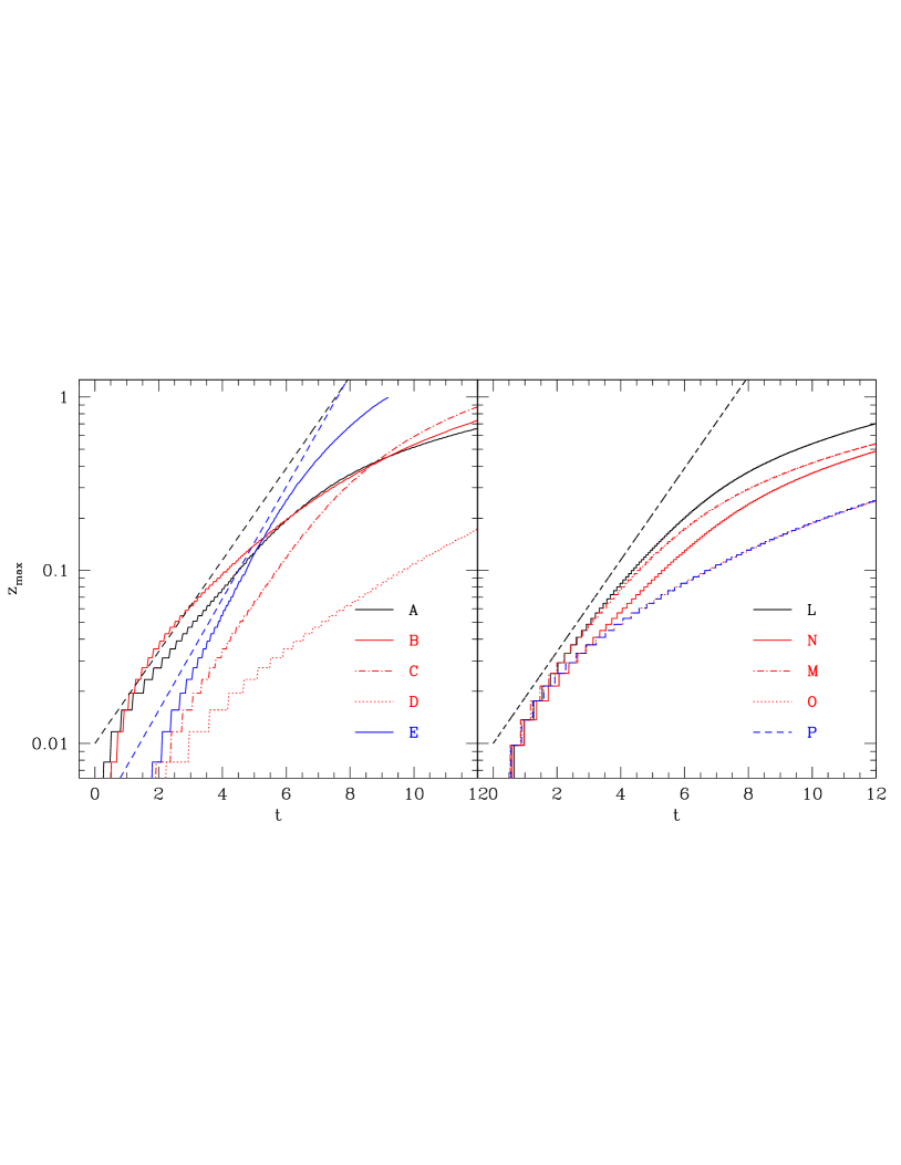
Figure 1.— Left: Growth of the vertical displacement $z_{\text{max}}$ between the top of the low density fluid bubbles and the initial interface due to RTI for different background states with a single mode perturbation given by eq. (11). Simulation parameters are listed in Table 1. The black and blue short dashed lines are the theoretical predictions from eq. (14) for interfaces with density ratios $\rho_{+}/\rho_{-}$ of $4$ and $16$, respectively. Right: The same as the left panel, except for simulations initially perturbed with the eigenvectors.

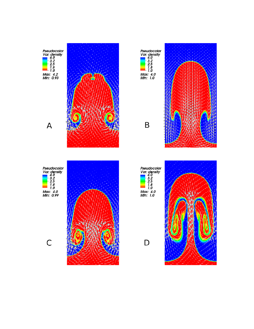
Figure 2.— Density and velocity field for the non-linear regime of RTI with a single mode perturbation. From left to right, top to bottom, the simulations are $A$ at time $8.8$, $B$ at time $14.0$, $C$ at time $11.6$ and $D$ at time $29.3$. Parameters of the simulations are listed in Table 1. The growth history of the four cases are shown in Figure 1. All the simulations adopt the Eddington approximation ${\sf\boldmath f}=1/3{{\sf\boldmath I}}$, which means the radiation pressure is assumed to be isotropic.

In addition to the density ratio at the interface, we anticipate that the behavior of RTI for radiation supported interface could differ depending on the background radiation properties, such as the ratio between radiation pressure and gas pressure and the characteristic optical depth. We proceed to vary these parameters and measure the growth rate from our simulations. We quantify the growth rate of RTI using $z_{\text{max}}$, the maximum distance of the interface from $z=0$. $z_{\text{max}}$ is measured by the perturbed regions that have density different from the initial density in those positions by at least $10\%$, such as the bubbles and fingers.

We first consider the case with single mode eigenvector perturbations. As discussed in the Appendix, we expect the growth rate consistent with eq. (14) since $\mathbb{C}\gg 1$ and the Eddington tensor is diagonal. The results are shown in the right panel of Figure 1. For a density ratio $\rho_{+}/\rho_{-}=4$ and wavenumber $k=2\pi$, eq. (14) predicts $z_{\text{max}}\propto\exp(0.61t)$, which is shown as solid line in the right panel of Figure 1. We find initial growth is faster than predicted for $z_{\text{max}}\lesssim 0.02$ (corresponding to $\lesssim 5$ cells). At such early times the vertical deformation of the interface is not well resolved and increases in the resolution improve agreement with constant growth rate solution. At later times, non-linear effects become important and the growth rate drops below the prediction for all runs, including the purely hydrodynamic case.

Although the curves are not uniformly consistent with exponential growth at a single constant growth rate, the range of growth rates inferred from the right panel of Figure 1 are close to the prediction of linear theory. Furthermore, many aspects of the linear theory are borne out by the results. Since $\mathbb{P}$ and $\kappa$ do not appear in eq. (14) the linear theory predicts no dependence on these parameters to first order in $\mathbb{C}^{-1}$. This is essentially correct for the initial stages of growth where the solutions remain in the linear regime. However, after about one sound crossing time in the simulations with large $\mathbb{P}$ and $\kappa$ ($N$, $O$, and $P$), the growth rate of $z_{\rm max}$ slows relative to the hydrodynamic and low $\mathbb{P}$ cases. This appears to be a non-linear behavior as the amplitude of the perturbation grows.

We attribute this non-linear behavior primarily to the effects of radiation drag, by which we mean that the fluid motions are damped by oppositely directed radiation forces. This requires that velocity fluctuations (on average) tend to directed opposite to the comoving radiation flux. Note that this is not equivalent to radiation viscosity, which is absent due to our assumption that the radiation field is isotropic (Mihalas & Mihalas, 1984). To linear order in perturbed quantities and lowest order in $\mathbb{C}^{-1}$, radiation drag is only relevant for compressible motions. The effects of radiation drag are most apparent in simulation where both $\mathbb{P}$ and $\kappa$ are large. Runs $O$ and $P$, with different values $\mathbb{P}$ and $\kappa$ but the same product of $\mathbb{P}\kappa$, follow similar trajectories. This is consistent with the linear analysis since the characteristic frequency $\nu\propto\mathbb{P}\kappa$ controls the importance of radiation drag on the solution. See the Appendix for further discussion.

The results of right panel of Figure 1 can be compared with the second set of single mode perturbations that are not eigenvectors, which are also shown in the left panel of Figure 1. In this case, a similar diversity of growth rates is observed, with notably reduced growth for the runs with larger $\mathbb{P}$ and $\kappa$. As with the eigenvector perturbations this trend of slower growth with larger radiation pressure appears to be a result of the radiation drag. In this case, the initial perturbations give rise to compressive motions which are largely absent in the eigenvector initial conditions. This allows radiation drag effects to become important at lower amplitude than in the eigenvector runs. But the range of late time (non-linear) evolution observed is qualitatively similar in the two sets of runs.

We have performed another simulation with the same parameters as simulation $D$, but with $\alpha=0$ i.e. with a background state supported by a gas pressure gradient instead of a radiation pressure gradient. We find a very similar growth history to that in simulation $D$. This confirms that the difference in the role of gas and radiation pressure in supporting the background has no qualitative effect on the resulting behavior. Radiation has relatively modest effects when $\mathbb{P}$ is small, but generically leads to slower growth when $\mathbb{P}$ and $\kappa$ are large. This strengthens the conclusion that damping of the compressible motions by radiation drag is the main effect of the radiation field. The fluid simply has more difficulty moving with respect to strong radiation field.

4.2. Non-linear structure with a single mode perturbation

The non-linear structure developed by RTI with single mode initial perturbations are shown in Figure 2, taken at late times in simulations $A-D$. By comparing the left two panels (simulation $A$ and $C$), we see that when the radiation pressure is comparable to the gas pressure and radiation pressure is assumed to be isotropic, RTI for the radiation supported interface and gas pressure supported interface have very similar non-linear structures. This is consistent with the fact that they have very similar linear growth phase as shown in Figure 1, especially when $\rho_{+}$ is increased to $16$ (simulation $E$).

The non-linear structures for the large radiation pressure cases (simulation $B$ and $D$) are quite different from simulations $A$ and $C$, especially at small scales. The Kelvin-Helmholtz (KH) instability, which is produced during the non-linear phase of RTI because of the shearing between the rising bubbles and falling fingers, is clearly damped in simulation $B$ where the optical depth across the box is $1$. When optical depth is increased to $10^{3}$ for simulation $D$, the small scale structures can survive because the size of those structures are much larger than photon diffusion length. However, these structures are still quite different when compared to the structures in simulations $A$ and $C$. The vortices are strongly stretched along the vertically direction when a strong radiation pressure exists.

4.3. Non-linear structures of RTI with random initial perturbations

To study the interactions between different modes of RTI, we add random perturbations to the vertical velocity as given by equation (12). As in section 4.2, the effect of radiation field on the RTI can be shown by comparing a set of controlled simulations ($F$, $G$, $H$, $I$, $J$), the parameters of which are listed in Table 1. The Eddington approximation is still used in those simulations.

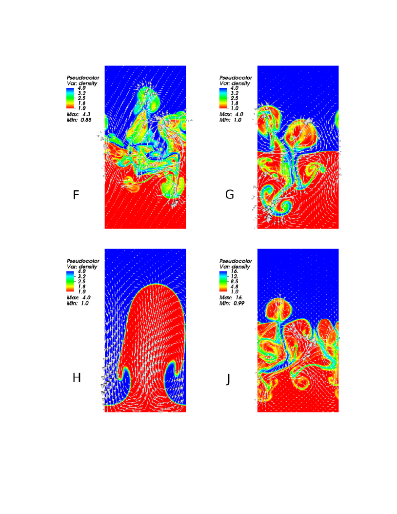
Figure 3.— Density and velocity field for the non-linear regime of RTI with random initial perturbations. From left to right, top to bottom, the simulations are $F$ at time $15.2$, $G$ at time $15.8$. $H$ at time $26.0$. $J$ at time $10.7$. All the simulations use the Eddington approximation. Parameters of the simulations are listed in Table 1.

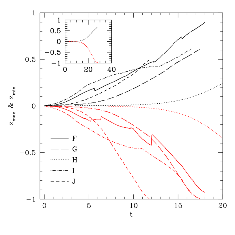
Figure 4.— Growth of vertical displacements $z_{\text{max}}$ and $z_{\text{min}}$ (the largest distance between the initial interface and the perturbed regions for $z>0$ and $z<0$ respectively) for RTI with random perturbations. The black (red) lines are for $z_{\text{max}}$ ($z_{\text{min}}$). Evolution over a longer time scale for simulation $H$ is shown in the left corner. Parameters of the simulations are given in Table 1.

In Figure 3, we show four snapshots from simulations $F,G,H,J$ (from left to right and from top to bottom) to illustrate the range of non-linear structures that we find. By comparing the top two panels ($F$ and $G$), we see that when radiation pressure is comparable to gas pressure ($\mathbb{P}=1$), the non-linear outcome of RTI for the radiation supported interface is similar to the case with gas pressure supported interface. There are two major differences when a radiation field is present. The first is that the dense, heavy fingers sink faster than the light bubbles rise up. This is not the case for the non-radiative RTI. Another difference is that for radiative RTI, the fluid is less mixed. In non-radiative RTI, there are many cells with density distributed between the whole range of the maximum and minimum density due to the small scale turbulence driven by secondary KH instabiity. However, with radiation field, there are fewer such cells. The result when $\rho_{+}$ is increased by a factor of $4$ is shown in the bottom right panel (simulation $J$). The mixing rate is increased as cells with intermediate densities occupy a larger fraction of the volume. The non-linear structures in this case bear more similarity to those in the purely hydrodynamic run. Recall that simulation $E$ has a linear growth rate very close to the growth rate of normal RTI, as shown in Figure 1. These results suggest that a higher ratio of $\rho_{+}/\rho_{-}$ reduces the impact of radiation and leads to behavior more consistent with the purely hydrodynamic RTI.

The effects of strong radiation pressure ($\mathbb{P}=10^{4}$, simulation H) on the non-linear structure is shown in the left bottom panel of Figure 3, where optical depth across the box along the horizontal direction is $1$. Due to the strong damping effect of the radiation field, all the small scale perturbations are damped and only the mode with the longest horizontal wavelength grows. In other words, the radiation field sets a minimum scale, above which the turbulence due to RTI can be sustained when radiation pressure is significant. Then the non-linear outcome is very similar to that in the runs with single mode perturbation with the same wavelength (simulation $B$ shown in Figure 2). The bubbles and fingers are well defined and mixing ratio is significantly reduced.

As in section 4.1, we use $z_{\text{max}}$ and $z_{\text{min}}$ to quantify the properties of RTI for the case with initial random perturbations. Here $z_{\text{min}}$ is similar to $z_{\text{max}}$ but only for the bottom half space ($z<0$) while $z_{\text{max}}$ is only for the top half space ($z>0$). Growth history for the five simulations ($F,G,H,I,J$) are shown in Figure 4. For non-radiative RTI (simulation $F$), the structure is symmetric with respect to the initial interface, which means $z_{\text{max}}$ and $z_{\text{min}}$ grow at approximately the same rate. However, this is not true for the RTI when a strong radiation field is present. As shown in Figure 4, for the case with radiation supported interface, $z_{\text{min}}$ reaches $-1$ at an earlier time than the time when $z_{\text{max}}$ reaches $1$. The asymmetry is reduced when opacity is increased (simulation $I$). The non-monotonic growth of $z_{\text{max}}$ and $z_{\text{min}}$ is likely caused by the mixing of the cells at the top of the bubbles and fingers. When the mixing is reduced (as in simulation H), the changes of $z_{\text{max}}$ and $z_{\text{min}}$ are always monotonic.

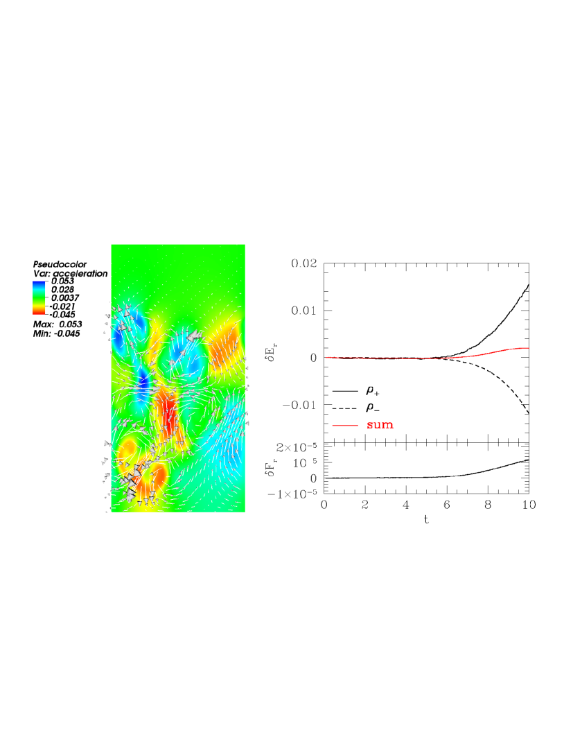
Figure 5.— Left: Snapshot of velocity (the vectors) and net acceleration (the color) due to radiation and gravity at time $t=15.8$ for simulation $G$. The corresponding density distribution at this time is shown in the top right panel of Figure 3. Right: The top panel shows the temporal evolution of the change of radiation energy density for low density fluid (dashed black line), high density fluid (solid black line) and total radiation energy density (red line) for simulation $G$. The bottom panel shows the change of the divergence of the flux across the whole simulation box compared with the initial value.

Figure 6.— Mixing ratio for the simulations with initial random perturbations. Parameters of the simulations are given in Table 1.

In the left panel of Figure 5, we show the net acceleration due to gravity and radiation flux along the vertical direction, $a_{\text{net}}=\mathbb{P}\kappa F_{r0,z}-g$, for simulation $G$ at time $15.8$. The initial hydrostatic equilibrium state has $a_{\text{net}}=0$ everywhere. The snapshot shows that for the bubbles moving up, $a_{\text{net}}>0$, which means that they are pushed up by the radiation force. For the falling fingers, $a_{\text{net}}<0$, which means that radiation force is not able to balance the gravity. The right panel of Figure 5 shows the history of the change of radiation energy density $\delta E_{r}$ and the divergence of the radiation flux across the whole simulation box $\delta F_{r}$ with respect to the initial values. Depending on whether the density in each cell is larger than $0.5(\rho_{+}+\rho_{-})$ or not, we can locate the regions containing high density fluid or low density fluid. The radiation energy density inside the high density fluid is increased because the high density fluid falls from the low radiation energy region to the high radiation energy region. The situation is inverted for the low density fluid. Because of the density (and, therefore, photon mean free path) difference, the radiation energy density of the low density fluid is changed more quickly than the high density fluid. Thus the bubbles lose the support from radiation force more quickly than the fingers and the asymmetry arises. When opacity is increased for the fingers, the photon mean free path is reduced and the diffusion time is longer.

When density contrast is increased by a factor of $4$ (simulation $J$), the growth rate is increased and the asymmetry is decreased. When radiation pressure is large enough ($\mathbb{P}=10^{4}$ for simulation H), the growths of $z_{\text{max}}$ and $z_{\text{min}}$ are significantly decreased, which is consistent with what we find for the single mode perturbation shown in section 4.1.

Figure 7.— Vertical profile of the initial $x-x$ ($f_{xx}$) and $z-z$ ($f_{zz}$) components of the Eddington tensor for the simulation G3 described in section 4.5. The Eddington tensor is invariant along the $x$ axis due to the symmetry of the initial condition. $f_{xx}$ decreases and $f_{zz}$ increases monotonically from the bottom to the top.

4.4. Mixing of the two fluids in the Rayleigh-Taylor Instability

With random perturbations, the non-linear regime of the RTI generates turbulence, in which there is significant mixing.

To quantify the degree of mixing, we count the number of cells with density between $90\%$ of the maximum density $d_{+}$ and $1.1$ times the minimum density $d_{-}$. The degree of mixing can be estimated by the ratio between the mixed cells and the total number of cells. The mixing ratio for the simulations with initial random perturbations is shown in Figure 6. For simulation $G$ with $\kappa=1$ and comparable gas pressure and radiation pressure, the mixing ratio is only $71\%$ of the mixing ratio for non-radiative RTI. When we increase the opacity to $\kappa=10^{3}$ (simulation $I$), the mixing ratio is very close to the case of non-radiative RTI because the photons are so tightly coupled to the fluid. When all the available modes are optically thick, the mixing that results from RTI is very similar in the radiative and non-radiative cases. However, if the smallest eddies are optically thin while the largest modes are optically thick, photons will decouple from the fluid on small scales and there will be less mixing on these scales. When radiation pressure is increased to $\mathbb{P}=10^{4}$, the mixing ratio is dropped to $\sim 8\%$. This is consistent with the fact that all the small scale structures are damped and KH instability, which is the most important cause of mixing the two fluids in normal RTI, is suppressed by the strong radiation field. We caution that we have not performed a numerical convergence study of mixing in the radiation RTI, and the precise mixing fractions we quote in this section are likely to change with numerical resolution. In fact, without explicit viscosity, converged results for the mixing rate are not possible. Nonetheless, the trends in the mixing rate with radiation pressure and opacity reported in this section should be independent of the viscosity and therefore numerical resolution.

4.5. Effects of Anisotropic Radiation Pressure

All the simulations listed in Table 1 adopt the Eddington approximation for the radiation field. Since the radiation pressure is assumed to be isotropic, these results only apply to very optically thick flows. We now consider cases with moderate to low optical depth and take into account the anisotropy of the radiation field by calculating VET self-consistently with equation (6). This allows us to assess the impact of anisotropic radiation pressure on the development of the RTI. Here we focus on the cases with a constant background radiation flux.

We first carry out a simulation G2 with Eddington approximation, which has almost the same setup as simulation G with a different initial perturbation. Here we perturb the density randomly as

$$\rho=\rho_{0}+\delta\rho(1+\cos(\pi z)),$$ (15)

where $\delta\rho$ is a random number uniformly distributed between $-0.5\rho_{0}$ and $0.5\rho_{0}$ and the perturbation is only applied when $|z|<0.5$. The initial radiation energy density at the bottom is $1.72$ and decreases to $0.22$ at the top due to the background radiation flux $F_{r,0}$, which balances the gravity. All the other initial conditions are the same as simulation G. A third simulation employing the VET is labeled as G3. Incoming specific intensities are applied at both the top and bottom of the box to maintain the same constant background flux $F_{r,0}$.

The initial vertical profile of the Eddington tensor is shown in Figure 7. For the pure scattering opacity case, the anisotropy is mainly caused by the stratification of the radiation energy density in order to provide the background radiation flux. From bottom to top, $f_{xx}$ decreases while $f_{zz}$ increases monotonically. The Eddington tensor changes vary rapidly within roughly one optical depth from the boundary and is close to $1/3$ in the middle of the simulation box. If we increase the vertical size of the simulation box, the profile of the Eddington tensor within one optical depth from the boundary remains the same while the middle region will become more isotropic. Not that we do not find $f_{xx}=f_{zz}=1/3$ at the bottom boundary because the downward going (backscattered) radiation field is not perfectly isotropic.

The growth history and mixing ratio of the two simulation G2 and G3 are shown in Figure 8. It is interesting to see that growth rate of G3 with VET is slower than the growth rate of G2. The mixing ratio from G3 is also smaller than the mixing ratio from G2. In Figure 9, we show snapshots of the non-linear structures to illustrate the differences between the two simulations. Consistent with Figure 8, there are more mixed (intermediate density) cells from simulation G2 and fewer in simulation G3. The top and middle panels in Figure 9 also show that the characteristic scale of eddies in G3 is larger than that of simulation G2. The slower growth rate in G3 is consistent with equation (14), which predicts that the growth rate of RTI decreases with decreasing wave number.

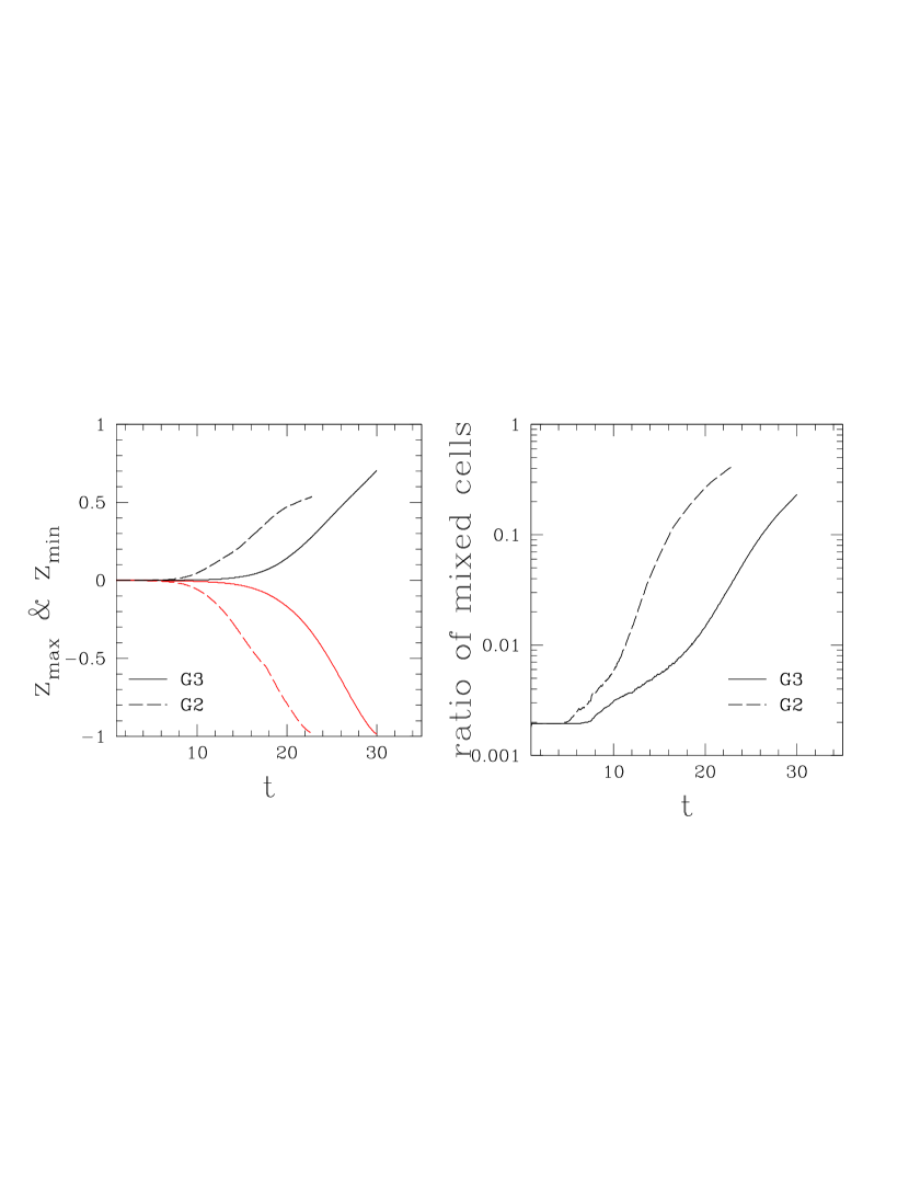
Figure 8.— Effects of VET on the growth rate and mixing ratio for RTI in a radiation supported interface. The left panel shows the evolution of $z_{\text{max}}$ and $z_{\text{min}}$ as in Figure 4 while the right panel shows the mixing ratio as in Figure 6. Simulation G2 adopts the Eddington approximation, while a VET is calculated self-consistently for simulation G3. All the other initial conditions are the same for the two simulations.

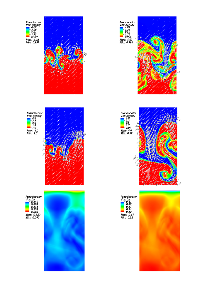
Figure 9.— Comparison of the non-linear structure from simulations G2 and G3, showing the effect of anisotropy in the radiation field captured through use of a VET. Top: Density distribution for G2 at time $15.2$ (left) and $21.6$ (right). Middle: Density distribution for G3 at time $21.6$ (left) and $28.9$ (right). The vectors in the those panels are the radiation flux with the background flux subtracted. Bottom: The horizontal ($f_{xx}$) and vertical ($f_{zz}$) components of the VET for simulation G3 at time $28.9$.

Components of the Eddington tensor $f_{xx}$ and $f_{zz}$ at the same time for simulation G3 are also shown in the two bottom panels of Figure 9. Interestingly, $f_{xx}$ and $f_{zz}$ actually have similar structures to the density distribution, which is also the photon mean free path distribution. There is a clear transition for the Eddington tensor between the fingers and bubbles: $f_{xx}$ is enhanced inside the finger while $f_{zz}$ is decreased compared with the initial values. Considering the complicated behavior of the Eddington tensor with position, it is not surprising that the non-linear structures produced by the RTI are different for simulations with VET and the Eddington approximation. Moreover, this result is a cause for concern regarding the reliability of results computed with much more approximate methods, such as flux-limited diffusion.

5. Radiation Supported Cold Shell

In ULIRGS, radiation from OB association is usually super-Eddington for adjacent dusty gas (e.g. Murray et al., 2005; Thompson et al., 2005; Krumholz & Matzner, 2009). The radiation field from these stars may have important feedback effects on the interstellar medium, such as reducing the star formation efficiency (e.g. Thompson et al., 2005) and driving the cold neutral outflows seen in many of these systems (Martin, 2005). Momentum driving may be more effective than thermal driving at accelerating clouds to escape velocities while not overheating and ablating the cold neutral gas (e.g. Murray et al., 2005; Martin, 2005; Socrates et al., 2008).

It has been recently argued (Krumholz & Thompson, 2012) that the RTI limits the ability of radiation pressure to support ULIRGs against gravity due to the temperature sensitivity of the dust opacity. Here we consider a related but somewhat different question of whether radiation pressure can effectively accelerate cold shells of gas before the RTI grows to a point that it limits radiative driving or provides enough mixing that the shell is no longer cold relative to the ambient medium.

Here we give a simplified two dimensional model to demonstrate the effects of RTI on the gas in the interstellar medium. Initially, a dense cold shell is in gas pressure equilibrium with surrounding hot gas. Gravity is balanced by the radiation pressure gradient. We assume pure constant scattering opacity so that we can start from an equilibrium state. Note that real dust can both absorb and scatter photons, with absorption opacity comparable to or slightly larger than scattering opacity at the temperature relevant for ULIRGS.

We adopt the parameters characteristic for ULIRGS (e.g. Thompson et al., 2005; Murray et al., 2005), subject to some constraints on the dynamical range that can be efficiently evolved by our simulation methods. The number density of the cold medium is $n_{c}=1000$ cm^-3, which corresponds to a mass density $\rho_{c}\sim 3.3\times 10^{-21}$ g cm^-3. The density ratio between the cold and hot medium is $100$. Temperature of the cold medium is $T_{c}=50$ K. The cold and hot gas are in gas pressure equilibrium. Gravitational acceleration is assumed to be $g=10^{-8}$ cm/s². A typical size scale is chosen to be $l_{0}\sim 1$ pc. With these parameters, the sound crossing time for $l_{0}$ is $\sim 10^{6}$ yr. To see the effects of varying the opacity, we try two different scattering opacities $1$ cm² g^-1 and $100$ cm^-2 g^-1 so that the optical depths across $l_{0}$ for the cold gas, which is labeled as $\tau_{s}$, are $0.01$ and $1$ respectively. Background radiation flux is chosen such that acceleration due to radiation force is $1.01$ times the gravitational acceleration. Thus, the cold shell will be accelerated upwards, representing the dusty gas which is pushed away by the strong radiation field. Taking $\rho_{c},T_{c}$ and $l_{0}$ as density, temperature and length units in our simulation, the dimensionless parameters $\mathbb{P}=8.1\times 10^{3}$ and $\mathbb{C}=7.10\times 10^{5}$.

The size of the simulation box is $l_{0}\times 4l_{0}$ and the cold shell is located at the middle, which extends from $-0.5l_{0}$ to $0.5l_{0}$. Periodic boundary conditions are used along the horizontal direction. For the vertical directions, density is fixed to be $0.01\rho_{c}$ in the ghost zones. The vertical components of the velocity and radiation flux in the ghost zones are fixed to the initial values while the horizontal components are copied from the last active zones. This vertical boundary condition can maintain the constant radiation flux entering and leaving the simulation box. Numerical resolution is $128\times 512$ for all the simulations.

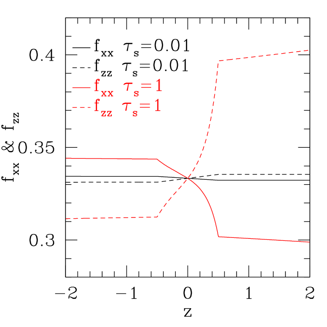
Figure 10.— Initial profiles of the $x-x$ and $z-z$ components of the Eddington tensor for the radiation supported cold shell shown in Section 5. The red lines are for the case when the optical depth across the cold shell is $1$ while the black lines are for the case with opacity $100$ times smaller. The rapid change in the Eddington tensor at positions $z=-0.5$ and $z=0.5$ are due to the jump in density (and, therefore, photon mean free path) at the interfaces. Although the density contrasts are $100$ for both the red and black lines, the change of Eddington tensor is much larger for $\tau_{s}=1$.

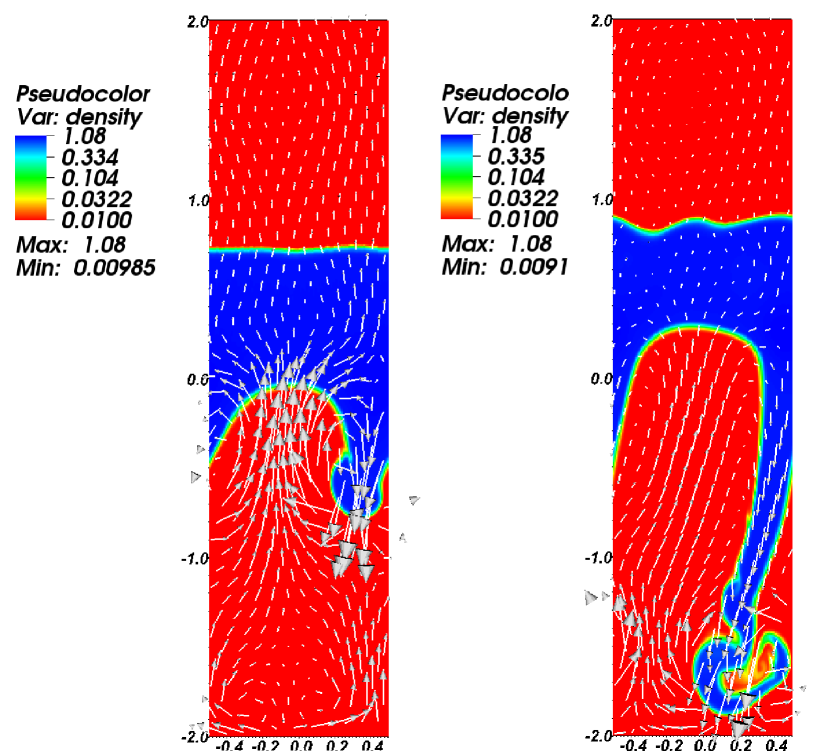
Figure 11.— Structures of the cold shell at times $2.3\times 10^{6}$ yr (left panel) and $1.1\times 10^{7}$ yr (right panel). Initial optical depth across the cold shell is $\tau_{s}=1$. Fingers and bubbles due to RTI are formed, which allows the cold dense gas to fall downwards instead of being pushed away by the background radiation flux. The vectors are the velocity field.

As discussed in section 4.5, to calculate the VET correctly, we find it is necessary to make the ratios of radiation flux to radiation energy density from the radiation transfer modules to be consistent with that obtained by evolving eqs. (4). The boundary conditions on the radiative transfer model enforce a constant flux and assume that the incoming intensity at the lower boundary is isotropic.

Given the density distribution and opacity, the initial VET is shown in Figure 10 for the two cases $\tau_{s}=0.01$ and $\tau_{s}=1$. When $\tau_{s}=1$, the cold shell is optically thick while the hot ambient medium is optically thin. Thus we see a rapid change of Eddington tensor near the interfaces at $z=\pm 0.5l_{0}$. The change is much smaller when $\tau_{s}=0.01$ and the radiation field remains nearly isotropic, consistent with the isotropy of the incoming radiation at the base of the domain. The vertical component of the Eddington tensor $f_{zz}$ increases with height while the horizontal component $f_{xx}$ decreases with height. Anisotropy of the radiation field is larger when $\tau_{s}=1$ and much smaller when $\tau_{s}=0.01$.

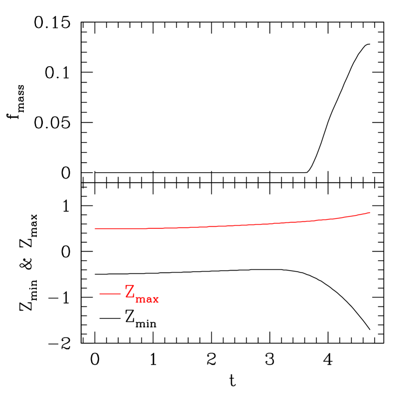
Figure 12.— Top: History of the fraction of cold dense gas that is below the line $-0.5l_{0}$. Time unit is $2.3\times 10^{6}$ yr. Before the RTI develops, no cold dense gas is below the line $-0.5l_{0}$ because the cold gas is pushed away by the radiation field. After RTI grows significantly, over $13\%$ of cold gas falls back during $\sim 2.8\times 10^{6}$ yr. Bottom: Change of the maximum and minimum heights of the cold dense gas with time. During the time $t<3.6$, the whole dense shell moves upwards. Once RTI grows significantly, some of the cold gas almost falls back to the bottom of the simulation box.

Initially, we perturb the density randomly according to equation 15. The random number $\delta\rho$ is uniformly distributed between $-0.005$ and $0.005$. As the acceleration due to the photons is $1\%$ larger than the gravitational acceleration in this setup, the whole shell will move upwards while RTI develops. The structure of the cold shell at times $2.3\times 10^{6}$ yr and $1.1\times 10^{7}$ yr for the case $\tau_{s}=1$ are shown in Figure 11. RTI develops quickly at the lower interface, where the high density medium is on top of the low density medium. The finger makes the cold dense gas fall back towards the low density gas exponentially, instead of being pushed away by the photons. In the top panel of Figure 12, we show how the fraction of cold gas that is below the line $-0.5l_{0}$, $f_{\text{mass}}$, change with time. Initially all the cold gas is located between $-0.5l_{0}$ and $0.5l_{0}$ and the whole shell is being pushed upwards before RTI develops, therefore $f_{\text{mass}}$ remains zero when $t<3.6$. After RTI grows significantly, $f_{\text{mass}}$ increases to $13\%$ after just $2.8\times 10^{6}$ yr. The maximum and minimum heights of the cold dense gas, $z_{\text{max}}$ and $z_{\text{min}}$, are shown at the bottom panel of Figure 12. Consistently with the history of $f_{\text{mass}}$, the whole shell moves upwards together during the time $t<3.2$. After $t=3.2$, $z_{\text{min}}$ decreases dramatically instead of increasing with time. The cold gas eventually reaches the bottom of the simulation box.

To see the effects of opacity, we decrease the opacity by a factor of $100$ so that $\tau_{s}=0.01$. In Figure 13, we show the density and velocity distribution at times $2.3\times 10^{6}$ yr and $1.1\times 10^{7}$ yr for this case. The evolution of the cold shell is quite different in this case compared with the case $\tau_{s}=1$, in that the two interfaces are both stable during the time when the shell crosses the simulation box. The whole shell is just pushed away by the photons and no cold gas is left.

By comparing Figure 11 and Figure 13, we can also see the different effect of radiation force in the optically thick and thin regimes. Initially in both cases, a constant radiation acceleration, which is larger than the gravitational acceleration, is applied across the shell to push it upwards. In the optically thin regime, the acceleration due to the radiation force is almost unchanged and it behaves like an effective gravitational acceleration. However, in the optically thick regime when RTI develops, the radiation flux is enhanced inside the bubbles and reduced inside the fingers. In this case the whole shell no longer moves with a constant acceleration. Instead, the cold gas falls back quickly through the fingers.

It is notable that the characteristic timescale for accelerating the shell $\sim\sqrt{2l_{0}/a}$, with $a\sim 0.01g$ is about $10^{7}$ years for the parameters under consideration. Since, the timescale for appreciable growth of the RTI is a few $\times 10^{6}$ years when $\tau_{s}\sim 1$, there is sufficient time for the RTI to grow and disrupt the shell. We have also performed runs with the radiation force is double the gravitational force, but keeping $\tau_{s}\sim 1$. This increases the effective acceleration by a factor of $\sim 100$ and reduces the timescale for acceleration to $\sim 10^{6}$ years. In this case the shell is accelerated efficiently and reaches the upper boundary of the domain before the RTI has time to grow appreciable. Hence we find that efficient acceleration of gas requires low optical depths or very super-Eddington radiation fluxes.

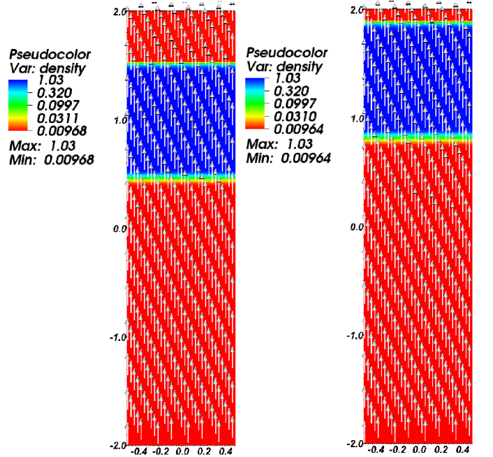
Figure 13.— The same as Figure 11 except that the initial optical depth across the cold shell is $\tau_{s}=0.01$ in this case. The two interfaces are both stable in this case and the whole cold shell is pushed upwards.

6. Summary and Discussions

Using our recently developed radiation hydrodynamic module for Athena, we have performed a set of numerical simulations to see the effects of strong radiation field on the development of the RTI for a background state with pure scattering opacity. In many respects, the radiative RTI is rather similar to the purely hydrodynamic RTI. Instability is always present when a high density fluid overlies a lower density fluid and we find growth rates that are within an order of magnitude of the hydrodynamic case, even when radiation pressure exceeds gas pressure by several orders of magnitude. Nevertheless, we find that the presence of radiation modified the development of the RTI in several significant ways.

For a gas pressure supported interface, the presence of a radiation field will generally reduce the growth rate of RTI, and growth rate decreases as the radiation pressure increases. This is because radiation acts as drag force when the material tries to move with respect to the radiation field. When radiation pressure is large ($\mathbb{P}\sim\mathbb{C}$), the development of small scale structure is also suppressed by the radiation field.

We find similar effects for a radiation pressure supported interface. In optically thick limit with an isotropic radiation field, the growth rate of the radiative RTI is similar to the non-radiative case. As we increase the radiation pressure and the opacity we find lower growth rates, which we again attribute to radiation drag effects. If the optical depth across the domain is low, so that the radiation becomes anisotropic, we generally find the growth rate is reduced relative to the isotropic case for the same parameters.

For a radiation supported interface with random perturbations, we find that it is easier for the dense fingers to sink than the light bubbles to rise up in contrast to the hydrodynamic RTI, where rising and sinking is nearly symmetric. This effect is more significant when opacity is decreased and the diffusion time across the fingers is reduced. The mixing process is also suppressed in radiation RTI, especially when radiation pressure is much larger than gas pressure.

The degree of radiation damping depends both on the opacity and the ratio between radiation pressure and gas pressure. When radiation pressure is large ($\mathbb{P}\sim\mathbb{C}$), all the modes will be affected by the radiation damping effect significantly as long as photons and gas are not decoupled for this mode. Turbulence due to RTI associated with secondary instabilities (e.g. Kelvin-Helmholtz) is significantly suppressed. When radiation pressure is just comparable to the gas pressure, only the small scale structures will be damped.

We have used a background state with pure scattering opacity because a background state with non-zero absorption opacity and an interface with a density discontinuity cannot generally obey both mechanical and thermodynamic equilibrium. This configuration will be particularly problematic in optically thick regime and the background state will evolve quickly because of the thermalization process. Any results obtained for systems with absorption opacity (e.g. Jacquet & Krumholz, 2011) will only be valid when the growth time of RTI is sufficiently shorter than the thermalization time or any other short timescale associated with the interface evolution (e.g. the evolution of an ionization front in an HII region).

In order to assess the effectiveness of radiative driving of cold gas outflows we simulate the acceleration of a cold, dense shell, for which radiation forces exceed gravity. We find that when the optical depth in the cold shell is $\sim 1$ and the radiation field is just slightly above Eddington, the RTI can develop quickly and prevent the acceleration of an appreciable amount of cold gas. However, if the radiation field is substantially super-Eddington, or if cold gas is very optically thin so that the growth rate of RTI is significantly reduced, the shell can be accelerated efficiently before the onset of the RTI. These simulations are too simplified to draw definite conclusions on the impact of RTI on radiation feedback in star forming environments, but suggest that the RTI is likely to be important in some cases. Those simulations also imply that if the growth time scale of RTI is smaller than the typical acceleration time scale, RTI is likely to change the structure of the system significantly. As we find that the growth rate of RTI is similar to normal RTI when radiation pressure is not significant ($\mathbb{P}\ll\mathbb{C}$) and the growth rate will be reduced when radiation pressure is very significant ($\mathbb{P}\sim\mathbb{C}$), our results give a general criterion on when RTI will be important when a specific astrophysical system is considered. Future work will benefit from the use of more realistic dust opacity and the use of non-grey (i.e. multiple frequency bins) radiative transfer to differentiate the impact of UV, mid-infrared, and far-infrared photons.

One caveat of our simulations is that they are done in 2D. It is known that RTI leads to different saturation states in 3D compared with 2D (e.g. Marinak et al., 1995). We plan to explore these effects on specific problems in future work. However, the linear growth rate is expected to be unchanged in 3D. We expect that the qualitative effects we find for the radiation field on the growth of the RTI, such as the importance of radiation drag in very radiation dominated regimes, will also be unchanged in 3D.

Other avenues for future research include studying the effects of absorption opacity on radiation RTI. If the thermal time scale is much longer than the growth time of RTI, we anticipate that absorption opacity will have minor effects on the growth and saturation of RTI. When the thermal time scale is much shorter than or comparable to the growth time of RTI, the effective equation of state of the fluid will be modified. Furthermore, the background state will also change dramatically in this case, which can also affect the saturation of RTI. The effects of absorption opacity on the RTI in specific astrophysic environments (e.g. with dust opacity in ULIRGS) is a topic of ongoing research that will be presented in future work. It is also important to include magnetic fields and examine the effects of radiation on magnetic RTI. Our radiation MHD code can also be used to study RTI in more specific astrophysical systems, such as H II regions with massive star formation, photosphere of accretion disks and supernova remnants.

Appendix A Linear Analysis

We present a simplified linear analysis of the Rayleigh-Taylor Instability in the case of a single interface between two constant density media with radiation, but in the limit of negligible absorption opacity. The background for this problem is described in Section 3 and specified by eqs. (7) - (10). We will consider the case with purely radiation support ($\alpha=1$) so the both density and gas pressure are constant within each half plane. The background is assumed to be static with ${{\mbox{\boldmath$F$}}_{r}}=F_{0}{\bf\hat{z}}$ and absorption opacity $\sigma_{s}=\kappa\rho$. With these assumptions, hydrostatic equilibrium reduces to $\mathbb{P}F_{0}\kappa=g$. We consider the 2D problem with a background that is uniform in x. Variables above and below the interface will be denoted by subscripts $+$ and $-$, respectively. We focus on the case with a diagonal Eddington tensor: $f_{xx}=f_{zz}=1/3$ and $f_{xz}=0$. Note that this assumption precludes radiation viscosity although still allows effects due to radiation drag (Mihalas & Mihalas, 1984).

We begin by linearizing eqs. (4) with perturbations of the form $f(x,z,t)=A(z)\exp\left[i(kx-\omega t)\right]$. We denote the $x$ and $z$ components of the velocity by $u$ and $w$, respectively. We denote the (scalar) radiation pressure by $P_{r}$ and the components of $x$ and $z$ components of $F$ by $F_{x}$ and $F_{z}$, respectively. Constant background quantities are denoted by a subscript zero, e.g. background density and vertical flux are denoted by $F_{0}$ and $\rho_{0}$. We then have:

$$-i\omega\delta\rho+\rho\left(iku+\frac{dw}{dz}\right) = 0,$$ (A1)

$$-i\omega\rho u+ika^{2}\delta\rho+-\mathbb{P}\sigma_{s}\delta F_{x}+\mathbb{P}\frac{4\sigma_{s}P_{r}}{\mathbb{C}}u = 0,$$ (A2)

$$-i\omega\rho w+a^{2}\frac{d\delta\rho}{dz}-\mathbb{P}\sigma_{s}\delta F_{z}+\mathbb{P}\frac{4\sigma_{s}P_{r}}{\mathbb{C}}w = 0,$$ (A3)

$$\frac{-3i\omega}{\mathbb{C}}\delta P_{r}+ik\delta F_{x}+\frac{d\delta F_{z}}{dz}+\frac{\sigma_{s}F_{0}}{\mathbb{C}}w = 0,$$ (A4)

$$\frac{-i\omega}{\mathbb{C}}\delta F_{x}+ik\delta P_{r}+\sigma_{s}\delta F_{x}-\frac{4\sigma_{s}P_{r}}{\mathbb{C}}u = 0,$$ (A5)

$$\frac{-i\omega}{\mathbb{C}}\delta F_{z}+\frac{d\delta P_{r}}{dz}+\sigma_{s}\delta F_{z}+\kappa F_{0}\delta\rho-\frac{4\sigma_{s}P_{r}}{\mathbb{C}}w = 0.$$ (A6)

Since the radiation field does not exchange any thermal energy with the gas when $\sigma_{a}=0$, gas energy equation simply reduces to a statement that gas pressure perturbation are adiabatic $\delta P=a^{2}\delta\rho$, with $a^{2}=\gamma P_{0}/\rho_{0}$. Note that since both $P_{0}$ and $\rho_{0}$ are constant, $a$ is a constant.

We further simplify the problem by selectively dropping terms of order $\mathbb{C}^{-1}$. In particular, we drop the time derivative terms in eqs. (A4)-(A6) and the fourth term on the rhs of eq. (A4). These terms are always small relative to other terms when $\mathbb{C}$ is large (i.e. the flow is non-relativistic). We nevertheless retain the last terms on the rhs of eqs. (A5) and (A6) because they include $P_{r}$, which can be much larger than $F_{0}$ in the limit of large optical depth. It is useful to first define a characteristic frequency

$$\nu=\frac{4P_{r}g}{F_{0}\mathbb{C}}=\frac{4P_{r}\kappa\mathbb{P}}{\mathbb{C}},$$

noting that this frequency generally varies with height, due to the linear dependence on the background $P_{r}$ on $z$.

We can use equations (A2) and (A5) to solve for $u$ and $\delta F_{x}$, obtaining

$$u=\frac{k}{\omega}\left(\frac{g\delta P_{r}}{\sigma_{s}F_{0}}+a^{2}\frac{\delta\rho}{\rho}\right),$$ (A7)

and

$$\frac{\delta F_{x}}{F_{0}}=-i\frac{k(\omega+i\nu)}{\omega}\frac{\delta P_{r}}{\sigma_{s}F_{0}}+\frac{\nu a^{2}k^{2}}{g\omega^{2}}\frac{\delta\rho}{\rho}.$$ (A8)

Inserting these into the above equations yields (after some algebra) a system of equations

$$\frac{dX}{dz}=AX$$

with

$$X^{\rm T}=\left(\frac{\delta P_{r}}{F_{0}},\frac{\delta F_{z}}{F_{0}},\frac{\delta\rho}{\rho_{0}},\xi\right)$$

and

$$A=\left(\begin{array}[]{cccc}0&-\sigma_{s}&-\sigma_{s}&-i\frac{\sigma_{s}\omega\nu}{g}\\ -\frac{k^{2}(\omega+i\nu)}{\sigma_{s}\omega}&0&-i\frac{k^{2}\nu a^{2}}{\omega g}&0\\ 0&\frac{g}{a^{2}}&0&\frac{\omega(\omega+i\nu)}{a^{2}}\\ \frac{k^{2}g}{\sigma_{s}\omega^{2}}&0&\frac{k^{2}a^{2}}{\omega^{2}}-1&0\end{array}\right).$$ (A13)

Here we have replaced $w$ by the Lagrangian displacement using the definition $w=-i\omega\xi$. These equations represent for ODEs, but with non-constant matrix coefficients i.e. the terms with $\nu$ vary with $z$. In what follows we will ignore this dependence and assume constant coefficients. Since $P_{r}=P_{0}-g\rho_{0}z$, $\nu$ is approximately constants for lengthscales $l\ll\mathbb{P}P_{0}/(g\rho_{0})$, Hence, it is a reasonable approximation for the subset of simulations with $\mathbb{P}\gg 1$.

With the above assumption, solutions take the form $\mathbf{\chi}^{i}_{\pm}\exp{(\lambda^{i}_{\pm}z)}$ with four eigenvalues $\lambda^{i}_{\pm}$. The eigenvalues for this system are given by

$$\left(\lambda^{2}-k^{2}\right)\left(\lambda^{2}-k^{2}+\frac{\omega(\omega+i\nu)}{a^{2}}\right)=0.$$

The first set of eigenvalues $\lambda^{2}=k^{2}$ have eigenvectors with $\delta P=a^{2}\delta\rho=0$ and

$$\frac{\delta F_{z}}{F_{0}} = -\frac{\omega(\omega+i\nu)}{g}\xi,$$

$$\mathbb{P}\delta P_{r} = \frac{\omega^{2}\rho}{\lambda}\xi.$$

These correspond to incompressible modes. The other set of compressible eigenvalues have $\lambda\pm\sqrt{k^{2}-\omega(\omega+i\nu)/a^{2}}$ and has eigenvectors with

$$\delta P = \frac{\rho\omega^{3}(\omega+i\nu)}{gk^{2}+\omega^{2}\lambda},$$

$$\mathbb{P}\delta P_{r} = \frac{\rho(g\omega^{2}\lambda-i\omega^{3}\nu)}{gk^{2}+\omega^{2}\lambda},$$

$$\delta F_{z} = -F_{0}\frac{k^{2}\omega(\omega+i\nu)}{gk^{2}+\omega^{2}\lambda}.$$

We now apply standard boundary conditions, the first being that the perturbations vanish far from the interface. The second set of conditions is given by matching solutions across the interface. In addition to the continuity of $w$, the non-trivial matching conditions come from integrating the vertical conservation relations in eqs. (4). As Jacquet & Krumholz (2011) discuss, these are equivalent to the continuity of the Lagrangian perturbations across the interface, which for our background correspond to

$$\mathbb{P}\Delta P_{r} = \mathbb{P}\delta P_{r}-\rho g\xi,$$

$$\Delta P = \delta P,$$

$$\Delta F_{z} = \delta F_{z}.$$

Defining perturbations above and below the interface proportional to

$$\chi^{\rm I}_{\pm}\exp{(\mp kz)}+\chi^{\rm C}_{\pm}\exp{(\mp\lambda_{\pm}z)},$$

where $\lambda_{\pm}$ correspond to the compressible eigenvalues and are both defined to have positive real parts. These matching conditions define a matrix $A\mathbf{X}=0$ with $\mathbf{X}^{\rm T}=\left(\chi^{I}_{+},\chi^{C}_{+},\chi^{I}_{-},\chi^{C}_{-}\right)$, and

$$A=\left(\begin{array}[]{cccc}1&1&-1&-1\\ 0&\frac{\rho_{+}}{\theta_{+}}&0&\frac{\rho_{-}}{\theta_{-}}\\ 1&\frac{k^{2}g}{\theta_{+}}&-1&-\frac{k^{2}g}{\theta_{-}}\\ \left(\frac{n^{2}}{gk}-1\right)\rho_{+}&-\frac{\rho_{+}}{\theta_{+}}\left(gk^{2}+\frac{i\omega^{3}\nu}{g}\right)&\left(\frac{n^{2}}{gk}+1\right)\rho_{-}&\frac{\rho_{-}}{\theta_{-}}\left(gk^{2}+\frac{i\omega^{3}\nu}{g}\right)\end{array}\right),$$ (A18)

where we have defined $\theta_{\pm}=gk^{2}\pm n^{2}\lambda_{\pm}$ and $n\equiv-i\omega$. The dispersion relation is obtained by setting $\det{A}=0$, which yields

$$\left(\lambda_{+}\rho_{-}+\lambda\rho_{+}\right)\left(-\frac{\omega^{2}}{gk}(\rho_{+}+\rho_{-})-(\rho_{+}-\rho_{-})\right)=0.$$

The quantity in the first set of parentheses has a real part which is always greater than zero. Hence if we look for purely imaginary solutions with growth rates $n\equiv-i\omega$, we obtain

$$n^{2}=gk\frac{\rho_{+}-\rho_{-}}{\rho_{+}+\rho_{-}}$$

which is equivalent to eq. (14), the standard result for the inviscid, incompressible hydrodynamic problem.

The robustness of this form for the dispersion relation may seem surprising, but is straightforward to understand. First note that the solution corresponds to the case where $\chi^{C}_{\pm}=0$ so the solution on either side of the interface is a purely proportional to the incompressible eigenvector. This result stems from the fact that only the purely incompressible eigenvectors permit the continuity of both $\delta F_{z}$ and $\delta P$ across the interface. In the limit that $\delta\rho=0$ and dropping the same $\mathbb{C}^{-1}$ terms as above, eqs. (A1)-(A6) reduce to

$$iku+\frac{dw}{dz}=0,$$

$$-i\omega\rho u+ik\mathbb{P}\delta P_{r}=0,$$

$$-i\omega\rho w+\mathbb{P}\frac{d\delta P_{r}}{dz}=0,$$

which resemble the hydrodynamics case, but with gas pressure perturbations replaced by radiation pressure. This should be contrasted with the optically thin case discussed by Jacquet & Krumholz (2011), where there is no $\delta P_{r}$ since the radiation field is decoupled from local conditions near the interface. In that case, since gravity is exactly balanced by radiation forces the effective gravity is zero and the interface is nominally stable.

Finally, we note that this result seems to imply that radiation drag have no effect on the linear growth rate. However, when $\nu$ is large ($\nu\gg\sqrt{gk}$), radiation drag forces make the linear regime of growth be rather limited. For large values of $\nu$, non-linear effects can become important, even for very modest velocity amplitudes. Indeed our numerical simulations indicate that non-linear effects become important at lower amplitudes for parameters corresponding to large $\nu$, as discussed in section 4.1.

References

- Andrews & Spalding (1990) Andrews, M. J., & Spalding, D. B. 1990, Physics of Fluids, 2, 922
- Chandrasekhar (1961) Chandrasekhar, S. 1961, Hydrodynamic and hydromagnetic stability, ed. Chandrasekhar, S.
- Dalziel (1993) Dalziel, S. 1993, Dynamics of Atmospheres and Oceans, 20, 127
- Davis et al. (2012) Davis, S. W., Stone, J. M., & Jiang, Y.-F. 2012, ApJS, 199, 9
- Dimonte et al. (2004) Dimonte, G., et al. 2004, Physics of Fluids, 16, 1668
- Jacquet & Krumholz (2011) Jacquet, E., & Krumholz, M. R. 2011, ApJ, 730, 116
- Jiang et al. (2012) Jiang, Y.-F., Stone, J. M., & Davis, S. W. 2012, ApJS, 199, 14
- Jun et al. (1995) Jun, B.-I., Norman, M. L., & Stone, J. M. 1995, ApJ, 453, 332
- Krolik (1977) Krolik, J. H. 1977, Physics of Fluids, 20, 364
- Krolik (2007) —. 2007, ApJ, 661, 52
- Krumholz et al. (2009) Krumholz, M. R., Klein, R. I., McKee, C. F., Offner, S. S. R., & Cunningham, A. J. 2009, Science, 323, 754
- Krumholz & Matzner (2009) Krumholz, M. R., & Matzner, C. D. 2009, ApJ, 703, 1352
- Krumholz & Thompson (2012) Krumholz, M. R., & Thompson, T. A. 2012, ApJ, 760, 155
- Kuiper et al. (2011) Kuiper, R., Klahr, H., Beuther, H., & Henning, T. 2011, ApJ, 732, 20
- Kuiper et al. (2012) —. 2012, A&A, 537, A122
- Lowrie et al. (1999) Lowrie, R. B., Morel, J. E., & Hittinger, J. A. 1999, ApJ, 521, 432
- Marinak et al. (1995) Marinak, M. M., et al. 1995, Physical Review Letters, 75, 3677
- Martin (2005) Martin, C. L. 2005, ApJ, 621, 227
- Marzec (1978) Marzec, C. J. 1978, PhD thesis, Columbia Univ., New York, NY.
- Mathews & Blumenthal (1977) Mathews, W. G., & Blumenthal, G. R. 1977, ApJ, 214, 10
- McKee & Ostriker (2007) McKee, C. F., & Ostriker, E. C. 2007, ARA&A, 45, 565
- Mihalas & Mihalas (1984) Mihalas, D., & Mihalas, B. W. 1984, Foundations of radiation hydrodynamics, ed. Mihalas, D. & Mihalas, B. W.
- Murray et al. (2005) Murray, N., Quataert, E., & Thompson, T. A. 2005, ApJ, 618, 569
- Schartmann et al. (2010) Schartmann, M., Burkert, A., Krause, M., Camenzind, M., Meisenheimer, K., & Davies, R. I. 2010, MNRAS, 403, 1801
- Sharp (1984) Sharp, D. H. 1984, Physica D Nonlinear Phenomena, 12, 3
- Shaviv (2001) Shaviv, N. J. 2001, MNRAS, 326, 126
- Socrates et al. (2008) Socrates, A., Davis, S. W., & Ramirez-Ruiz, E. 2008, ApJ, 687, 202
- Spiegel & Tao (1999) Spiegel, E. A., & Tao, L. 1999, Phys. Rep., 311, 163
- Stone & Gardiner (2007a) Stone, J. M., & Gardiner, T. 2007a, Physics of Fluids, 19, 094104
- Stone & Gardiner (2007b) —. 2007b, ApJ, 671, 1726
- Thompson et al. (2005) Thompson, T. A., Quataert, E., & Murray, N. 2005, ApJ, 630, 167
- Turner et al. (2005) Turner, N. J., Blaes, O. M., Socrates, A., Begelman, M. C., & Davis, S. W. 2005, ApJ, 624, 267