Open windows for a light axigluon explanation of $A_{FB}^{t}$

Abstract

The top forward-backward asymmetry ($A_{FB}^{t}$) measured at the Tevatron remains one of the most puzzling outstanding collider anomalies. After two years of LHC running, however, few models for $A_{FB}^{t}$ remain consistent with LHC data. In this paper we take a detailed look at the most promising surviving class of models, namely light ($m_{G^{\prime}}\lesssim 450$ GeV), broad axigluons. We show which models simultaneously satisfy constraints from Tevatron and LHC top measurements, hadronic resonance searches, and LEP precision electroweak (PEW) observables. We consider three flavor structures: flavor-universal; down-type nonuniversal, designed to ease constraints from LHC charge asymmetry measurements; and top-type nonuniversal, designed to ameliorate constraints from PEW. We compute contributions to the PEW observables from states in the minimal UV completion of the axigluon model and demonstrate that new heavy fermions make the constraints universally more stringent, while related contributions from new scalars are much smaller, but act to relax the constraints. Paired dijet searches from ATLAS and CMS rule out all narrow axiglue models, while the LHC charge asymmetry measurement is less constraining than expected due to the high central value measured by ATLAS. Excepting the tension with the CMS charge asymmetry measurement, a broad axigluon is consistent with all data over the entire mass range we consider ($50\mbox{ GeV}\lesssim m_{G^{\prime}}\lesssim 450\mbox{ GeV}$) in the flavor-universal and top-type nonuniversal models, while it is consistent for $m_{G^{\prime}}\gtrsim 200\mbox{ GeV}$ in the down-type non-universal model. The LHC charge asymmetry remains the best avenue for excluding, or observing, these models.

I Introduction

The anomalously large measurement of the top forward-backward asymmetry $A_{FB}^{t}$ at the Tevatron is one of the most significant and puzzling outstanding collider anomalies. The CDF and D0 collaborations have independently measured inclusive asymmetries approximately $2\sigma$ above the Standard Model (SM) expectation; the most recent measurements are detailed in Table 1 Aaltonen et al. (2012); Abazov et al. (2011). In addition, both experiments have observed more significant discrepancies between measurement and SM predictions in subsystems of the $t\bar{t}$ events. Interest in the $A_{FB}^{t}$ exploded after CDF’s 5.3 fb^-1 measurement Aaltonen et al. (2011a) of a $A_{FB}^{t}=0.475\pm 0.114$ asymmetry in events with $M_{t\bar{t}}>450\text{GeV}$, which was 3.4$\sigma$ above the SM prediction at the time. In the updated measurement using the full CDF data set, the high-mass excess has been mitigated, but still grows very steeply with center of mass energy, and is 2.3 $\sigma$ above the SM expectation Aaltonen et al. (2012). Unfortunately D0 does not unfold their differential $A_{FB}^{t}$ measurement, so it is not possible to directly compare their results in the high invariant mass range to those of CDF. D0 does, on the other hand, measure the lepton asymmetry in $t\bar{t}$ events, which provides a clean and theoretically sensitive cross check of the parent top asymmetry Bernreuther and Si (2010); Krohn et al. (2011). D0 finds, in 5.4 fb^-1, at production level $A^{\ell}_{FB}=15.2\pm 4.0\%$, which is more than 3$\sigma$ above the MC@NLO prediction of $A^{\ell}_{FB,SM}=2.1\pm 0.1\%$ Abazov et al. (2011). However, the significance of this result has also been reduced with the addition of more data. Combining with measurement of the (single) lepton asymmetry in dileptonic top events, and including EW contributions in the SM prediction, the updated result for the D0 single lepton asymmetry is reduced to $A^{\ell}_{FB}=11.8\pm 3.2\%$, a 2.2$\sigma$ discrepancy with the SM Abazov et al. (2012). Meanwhile, CDF finds a $2\sigma$ excess from the SM in the background-subtracted $A_{FB}^{\ell}=6.6\pm 2.5\%$ with a SM prediction of $1.6\%$ The CDF Collaboration (2012).

While the deviation from SM predictions for the inclusive top forward-backward asymmetry does not have high significance, the consistency of the excess both across time and across experiments is a possible indication of a non-statistical origin for the asymmetry. The mystery is deepened by the excellent agreement of other top properties with the predictions of the SM, and in particular by the consistency of the $t\bar{t}$ production cross-section (both inclusive and differential) between theory and experiment.

$M_{t\bar{t}}$	$A_{FB}^{t}$	Measurement/Prediction at Parton Level
inclusive	$0.164\pm 0.045$	CDF Aaltonen et al. (2012)
	$0.196\pm 0.065$	D0 Abazov et al. (2011)
	$0.066\pm 0.020$	POWHEG SM prediction after applying EW corrections Aaltonen et al. (2012)
$>450$ GeV	$0.295\pm 0.058\pm 0.031$	CDF Aaltonen et al. (2012)
	$0.100\pm 0.030$	POWHEG SM prediction after applying EW corrections Aaltonen et al. (2012)
	$A_{FB}^{\ell}$
	$0.152\pm 0.04$	D0 Abazov et al. (2011)
	$0.118\pm 0.032$	D0, dileptonic & semileptonic, combined Abazov et al. (2012)
	$0.047\pm 0.001$	(D0) MC@NLO plus EW Abazov et al. (2012)
	$0.066\pm 0.025$	CDF, background subtracted The CDF Collaboration (2012)
	$0.016$	(CDF) NLO (QCD + EW) The CDF Collaboration (2012)

Table 1: Recent measurements of $A_{FB}^{t}$ and $A_{FB}^{\ell}$ along with SM predictions.

Very many new physics models have been proposed to explain the anomalously large top asymmetry. Most have addressed the tension between the discrepant $A_{FB}$ and the well-behaved cross-section by deferring predicted deviations in the spectrum to partonic center of mass energies beyond the Tevatron’s reach. For heavy $s$-channel particles such as axigluons Frampton et al. (2010); Chivukula et al. (2010); Bai et al. (2011); Haisch and Westhoff (2011); Gresham et al. (2011a); Barcelo et al. (2012); Alvarez et al. (2011), which have large masses $m\lower 3.01385pt\hbox{$\;\stackrel{{\scriptstyle\textstyle>}}{{\sim}}\;$}$TeV as well as broad natural widths $\Gamma\lower 3.01385pt\hbox{$\;\stackrel{{\scriptstyle\textstyle>}}{{\sim}}\;$}0.3\,m$, significant deviations from SM predictions for the dijet and top pair spectra are inevitable at and above a TeV, as center of mass energies begin to approach the axigluon pole. Meanwhile models that generate the asymmetry via the $t(u)$-channel exchanges of flavor-violating/carrying vectors (scalars) Jung et al. (2010); Shu et al. (2010); Gresham et al. (2011b); Shelton and Zurek (2011); Jung et al. (2011a, b) typically involve mediators significantly lighter than a TeV with large, flavor off-diagonal couplings. These models attain reasonable agreement with Tevatron top cross-sections by arranging a cancellation between interference and new-physics terms at Tevatron energies. This cancellation no longer holds at LHC energies, so while these models do avoid producing a dijet or $t\bar{t}$ resonance, the high-$m_{t\bar{t}}$ tail in top pair production is strongly enhanced (suppressed) Gresham et al. (2012a); Delaunay et al. (2011); Aguilar-Saavedra and Perez-Victoria (2011a). Models with sufficiently light and weakly coupled mediators $M$ can avoid over (under)-producing $t\bar{t}+X$; however, the large single top production in these models, $t+M\to t+jj$, contributes at unacceptable levels to top pair cross-section analyses. Moreover, processes in which the mediators are directly produced on-shell in association with the top quark lead to many distinctive and charge-asymmetric processes that contribute to single top and top pair final states Craig et al. (2011); Knapen et al. (2012). Top-jet resonances arise in these models Gresham et al. (2011b), which have been searched for and excluded over much of the parameter space Chatrchyan et al. (2012a); ATLAS (2012). Top cross-section measurements at the LHC thus exclude these classes of models when all contributions to top-pair-like final states are taken into account, unless additional BSM decay modes for the mediator are introduced to hide it Alvarez and Leskow (2012); Drobnak et al. (2012a). $t(u)$-channel models are also strongly constrained by low-energy Atomic Parity Violation (APV) measurements Gresham et al. (2012b) and the failure of the LHC experiments to observe large charge asymmetries Aguilar-Saavedra and Perez-Victoria (2011a); Aad et al. (2012); Chatrchyan et al. (2012b) or deviations from SM predictions in top polarization and spin correlations Fajfer et al. (2012).

As the LHC has thus far failed to find significant deviations from standard model predictions for single top or $t\bar{t}$ processes, using heavy new states to explain the top forward-backward asymmetry is now increasingly disfavored Delaunay et al. (2012). Only small regions of parameter space remain for heavy axigluons with the top quark coupling much larger than light quark coupling to evade dijet constraints.

As an alternative approach, new physics explanations for the top forward-backward asymmetry can instead invoke light axigluons Tavares and Schmaltz (2011); Aguilar-Saavedra and Perez-Victoria (2011b); Krnjaic (2012); Drobnak et al. (2012b), which can be more weakly coupled and therefore lead to much smaller deviations from SM predictions for top properties. Here by “light” axigluons, we mean models where the light quark and top quark axial couplings have the same sign, $\text{sign}(g_{A}^{q})=\text{sign}(g_{A}^{t})$. In order to generate the observed sign for the inclusive forward-backward asymmetry, these axigluons must therefore be not much heavier than $\sim 2m_{t}$. These light axigluons would be copiously produced at current and past colliders, and require model building to be “hidden” from discovery under large QCD backgrounds.

We will examine the existing constraints on light, hidden axigluons and related particles. Direct collider searches for narrow resonances decaying to dijets entirely eliminate narrow axigluons above 100 GeV. Below the $Z$ pole axigluons run into constraints from the running of $\alpha_{s}$, and are excluded for masses below approximately 50 GeV Kaplan and Schwartz (2008). For sufficiently broad and weakly coupled axigluons, it is possible to avoid discovery in direct collider searches. In these cases the most important constraints come from two indirect measurements. First, the one-loop axigluon corrections to the $Z\rightarrow q\bar{q}$ coupling constrains light axigluon models through the LEP precision electroweak (PEW) measurements of the hadronic $Z$ width and the total hadronic cross-section at the $Z$ pole Haisch and Westhoff (2011). Second, the non-observation of a large charge asymmetry at the LHC is also becoming constraining for light axigluons Drobnak et al. (2012b). These indirect constraints are highly sensitive to the flavor structure of the axigluon-quark couplings. As we will see, the constraints from PEW observables and from the LHC charge asymmetry measurements make competing demands on the flavor structure, which significantly limit the allowed parameter space.

We will discuss three flavor structures. First, we consider flavor-universal axigluons. Second, we consider axigluons where the coupling to right-handed down-type quarks is enhanced, a choice which helps to reconcile LHC and Tevatron charge asymmetry measurements Drobnak et al. (2012b), but exacerbates the tensions with PEW observables. Third, we consider axigluons with an enhanced coupling to top quarks, a choice motivated by minimal flavor violation-type models and models with a special role for the third generation, which alleviates the tension with the PEW observables but does not help with the LHC charge asymmetry measurement. These models also can run into difficulty with the lepton asymmetry measured at the Tevatron.

The outline of this paper is as follows. In the next section we present an overview of the Tevatron forward-backward and LHC forward-central charge asymmetry measurements and identify two interesting non-minimal flavor structures that are safe from low-energy precision measurements. We then summarize existing constraints on light axigluons from top pair production that are largely independent of the axigluon width: the forward-backward and forward-central charge asymmetries in section III.1, the lepton asymmetry in section III.2, and total cross-section in III.3. We discuss constraints from direct collider searches, in particular from paired dijets, in section IV. Precision EW constraints for both the axigluon alone and for various extensions of the broad axigluon model are considered in section V. Finally we assemble the constraints and perform a global fit, identifying surviving regions in parameter space. We refer the reader to Figs. 10, 11 for a summary of the open windows for a light axigluon explanation of $A_{FB}^{t}$. While this work was in preparation, Gross et al. (2012) appeared, which has overlap with this work.

II Models and Conventions

In this section we define a minimal reference Lagrangian for a light axigluon and discuss the three flavor structures we will focus on. We describe the axigluon as arising from a spontaneous breaking of $SU(3)_{1}\times SU(3)_{2}\to SU(3)_{c}$. This is the minimal renormalizable realization of a massive vector octet, and gives the Lagrangian for the axigluon $G^{\prime}$ and SM gluon $G$:

$$\mathcal{L}=-\frac{1}{4}(D_{\mu}{G^{\prime}}_{\nu})^{a}(D_{\mu}{G^{\prime}}_{\nu})^{a}-{g_{s}\over 2}\chi\,f^{abc}\,G^{\mu\nu a}{G^{\prime}}_{\mu}^{b}{G^{\prime}}_{\nu}^{c}$$ (II.1)

where

$$(D_{\mu}{G^{\prime}}_{\nu})^{a}=\partial_{\mu}{G^{\prime}}_{\nu}+g_{s}f^{abc}G^{b}_{\mu}{G^{\prime}}_{\nu}^{c}-(\mu\leftrightarrow\nu).$$ (II.2)

and the coefficient of the second term in Eq. II.1, which in the low-energy theory is undetermined, is fixed in the UV completion to be $\chi=1$.

Axigluon couplings to quarks,

$$\mathcal{L}=-\sum_{i=1}^{3}\left(g_{L,i}\bar{Q}_{L}^{i}\not{G^{\prime}}Q_{L}^{i}+g_{R,i}^{D}\bar{d}_{R}^{i}\not{G^{\prime}}d_{R}^{i}+g^{U}_{R,i}\bar{u}_{R}^{i}\not{G^{\prime}}u_{R}^{i}\right),$$ (II.3)

on the other hand, are model-dependent. In general, axigluon-quark couplings $g_{i}$ smaller than $g_{s}$ are necessary for light axigluons to give a good fit to the Tevatron data. Since simple embeddings of the quark generations into the minimal UV group $SU(3)_{1}\times SU(3)_{2}$ give axial couplings bounded from below by $g_{s}$, the small couplings needed to explain the Tevatron data are challenging to obtain without invoking new degrees of freedom Tavares and Schmaltz (2011); Cvetic et al. (2012), as summarized in appendix A. Our standpoint here will be purely phenomenological, using a simple low-energy Lagrangian with freely-adjustable couplings between axigluons and quarks. However, as the structure of the minimal UV completion is sharply defined, and as some of the additional degrees of freedom could provide natural additional decay channels for the axigluon, we will also consider contributions to PEW observables from additional heavy degrees of freedom in Section V.

We concentrate on three patterns for the quark-quark-light axigluon couplings that are compatible with flavor constraints without fine-tuned alignment of mass and flavor bases. We consider the Lagrangian,

$$\mathcal{L}=-\left(g_{L}\bar{Q}_{L}^{i}\not{G^{\prime}}Q_{L}^{i}+g^{D}_{R}\bar{d}_{R}^{i}\not{G^{\prime}}d_{R}^{i}+g^{U}_{R}\bar{u}_{R}^{i}\not{G^{\prime}}u_{R}^{i}+\delta^{t}_{R}\bar{t}_{R}\not{G^{\prime}}t_{R}\right).$$ (II.4)

with the four parameters $g_{L},g^{D}_{R},g^{U}_{R},\delta^{t}_{R}$ occurring in the combinations given in Table 2. This defines three flavor scenarios: (i) flavor universal Tavares and Schmaltz (2011); Krnjaic (2012) (ii) down-type non-universal Drobnak et al. (2012b); Aguilar-Saavedra and Juste (2012) and (iii) top non-universal. The down-type non-universal scenario is preferred by CMS LHC charge asymmetry measurements, and the top non-universal scenario is preferred by PEW measurements. In all three scenarios, couplings to up quarks are chosen to be purely axial ($g_{A}={1\over 2}(g_{R}-g_{L})\neq 0,\;g_{V}={1\over 2}(g_{R}+g_{L})=0$), since this is the choice that maximally affects top charge asymmetries while minimizing the effect on charge-symmetric top observables. We consider enhancement of only the RH top coupling (not RH bottom or LH top-bottom doublet) because it is motivated by minimal flavor violation and—more importantly—because constraints are weakest: constraints on models with $b$ coupling enhancement as well would only increase. Axigluons with mass below the top quark require very moderate couplings in order to generate a charge asymmetry commensurate with the measured Tevatron values and are therefore typically narrow if their only allowed decays are to quarks. Since dijet resonance constraints rule out most such models, we consider both narrow and broad axigluons. For concreteness we will take 20% as a benchmark “broad” width and the natural width to light quarks as a “narrow” width.

Scenario Name	Couplings
Flavor universal	${g_{R}^{U}}=g_{R}^{D}=-g_{L}\equiv g_{A};\;\delta^{t}_{R}=0$
Down-type non-universal	${g_{R}^{U}}=-g_{L}\neq g_{R}^{D};\;\delta^{t}_{R}=0$
Top non-universal	${g_{R}^{U}}=g_{R}^{D}=-g_{L}\equiv g_{A};\;\delta^{t}_{R}=g^{t}_{R}-g^{U}_{R}\neq 0$

Table 2: Definitions of the axiglue scenarios we consider.

An axigluon with large enough couplings to light quarks and the top quark to generate the asymmetry at the Tevatron must satisfy several non-trivial constraints. We outline the constraints we will detail below for the three classes of axiglue models we consider.

(1) Flavor Universal:

• LHC charge asymmetry. For narrow and broad axigluons, the Tevatron and LHC charge asymmetry as measured by CMS are in mild tension for the entire mass range. However, the ATLAS charge asymmetry is perfectly commensurate with Tevatron $A_{FB}^{t}$.

• Precision electroweak (PEW) constraints, dominantly from one-loop corrections to the $Z$-$q$-$\bar{q}$ vertex. These constraints strongly disfavor a sub-100 GeV narrow or broad axigluon.

• Single and paired dijet constraints. Narrow axigluons are strongly disfavored by single dijet resonance searches at hadron colliders in all but the sub-$m_{Z}$ mass range. Paired dijet searches also rule out the entire narrow resonance window from constraints on production of two axigluons that decay to pairs of jets.

As we will show, these combined constraints leave a strip of parameter space open for a light flavor universal axigluon heavier than $m_{Z}$. A lower charge asymmetry measurement from ATLAS would strengthen the constraints on these models considerably. Individual constraints can be partially or fully alleviated in flavor non-universal models. Constraints from a low LHC charge asymmetry can be alleviated by increasing couplings to down-type quarks Kamenik et al. (2011). Precision electroweak constraints can be relaxed by allowing the light quark couplings to be small by simultaneously increasing the top quark couplings. Paired dijet constraints still eliminate all flavor non-universal models with a narrow axigluon; broad axigluons survive.

(2) RH Up-Down Flavor non-Universal Axigluons:

• By taking the coupling to the down quark larger than to the up-type quarks, constraints from the CMS LHC charge asymmetry can be eliminated.

• Precision electroweak constraints are particularly stringent in this case, requiring the axigluon to be heavier than 200 GeV.

• Even though alleviating the tension with the CMS LHC charge asymmetry requires RH down-type quark couplings of order $g_{s}$, the consequent increase in the Tevatron top pair cross-section is still small.

• As for all flavor choices, paired dijet constraints eliminate narrow axigluons over the entire mass range. For this case, broad axiglue are also constrained by UA1 dijets.

(3) RH Top non-Universal Axigluons:

• These models do nothing to alleviate the CMS LHC charge asymmetry constraint.

• By taking the coupling to RH top much larger than that to the light quarks, precision electroweak constraints are alleviated.

• These models can over-predict the Tevatron lepton asymmetry, particularly for axigluons below the $2m_{t}$ threshold.

In the following sections we discuss in depth the observables and constraints for each of the above-mentioned scenarios.

III Top pair observables

We begin by identifying the parameter ranges that produce sufficiently large asymmetries at the Tevatron and illuminate any tension with other $t\bar{t}$ observables such as the LHC charge asymmetry and the $t\bar{t}$ cross-section. We also discuss the Tevatron lepton asymmetry constraints on these scenarios, which can be important for large non-universal axigluon couplings to $t_{R}$.

III.1 Tevatron $A_{FB}^{t}$ and LHC $A_{C}^{t}$

The charge asymmetry at the LHC $A_{C}^{t}$ is highly correlated with the forward-backward asymmetry $A_{FB}^{t}$ at the Tevatron, and provides one of the most direct cross-checks of the Tevatron measurement. The current situation for $A_{C}^{t}$ at the LHC is rather unclear. $A_{C}^{t}$ as measured by ATLAS in dileptonic events, $A_{C}^{t}=0.057\pm 0.024\pm 0.015$, differs by more than a standard deviation from the CMS measurement using semileptonic events, $A_{C}^{t}=0.004\pm 0.01\pm 0.012$. The two collaborations are more consistent if the semileptonic result from ATLAS with $1/4$ the data is included. For this reason, the $A_{C}$ constraint from the LHC is not as strong as expected by this point from the data.

Figs. 1 and 2 show $A_{FB}^{t}$ and $A_{C}^{t}$ for light axigluon models in all three flavor structures. The contributions to $A_{FB}^{t}$ and $A_{C}^{t}$ due to leading order (LO) new physics are shown for various choices of parameters alongside CDF and D0 bands corresponding to the measured asymmetry minus the standard model expectation as reported by the collaboration, with errors given by the experimental and SM prediction uncertainties added in quadrature. We assume linear addition of SM and BSM contributions to the asymmetry. Following CDF, we multiply D0’s reported QCD-only SM prediction by 1.26 to account for EW corrections and include a $30\%$ error on the SM expectation. We use QCD predictions as reported by the experiments, though there is some concern that these predictions are underestimates Manohar and Trott (2012). Calculations are semi-analytic. We used CTEQ5 parton distribution functions with $m_{t}=173$ GeV and set the renormalization and factorization scales to $m_{t}$; sensitivity to the renormalization/factorization scales was checked by varying scales between $m_{t}/2$ and $2m_{t}$. Flavor-universal couplings are in tension with the CMS result, but not the ATLAS result. Down-type non-universal models can provide a better fit to $A_{FB}^{t}$ and a lower $A_{C}^{t}$ Drobnak et al. (2012b), while top non-universal models do not alleviate the tension between $A_{FB}^{t}$ and $A_{C}^{t}$.

Flavor universal	Flavor universal
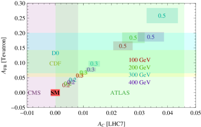
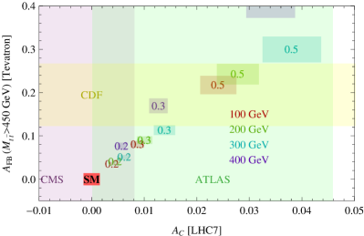
Down-type non-universal	Top non-universal

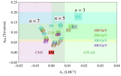
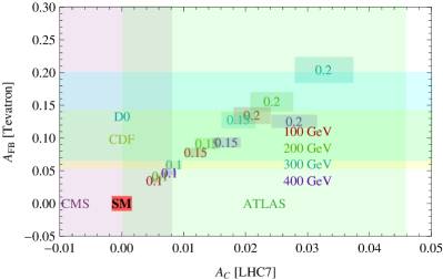
Figure 1: Asymmetries in $q\bar{q}\rightarrow t\bar{t}$ events ($t\bar{t}j$ events are a minor correction and not included here) for axigluon models with masses 100, 200, 300, and 400 GeV. Widths have been set to 20%, though the asymmetries are insensitive to variations of width between 1% and tens of percent for masses below $2m_{t}$. Plot markers indicate $g_{R}^{U}=-g_{L}$ in units of $g_{s}$. Down-type universal models shown have $g_{R}^{D}=-ng_{R}^{U}$ and the top non-universal model shown has $g_{R}^{t}=10g_{R}^{U}$. Shaded rectangles behind plot markers show the variation in $A_{FB}^{t}$ and $A_{C}^{t}$ for factorization/renormalization scales varying from $m_{t}/2$ to $2m_{t}$. The most recent CDF (light yellow), D0 (cyan), CMS (light purple), and ATLAS (dileptonic + semileptonic combination, light green) 1$\sigma$ bands are shown. The bands are centered on the central value minus the SM NLO expectation as reported by each collaboration.

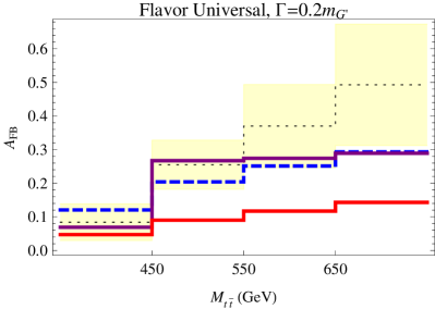
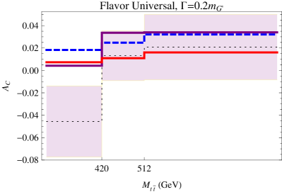
Figure 2: Asymmetries binned according to $M_{t\bar{t}}$ for a 200 (dashed blue) and 400 (solid purple) GeV axigluon with universal coupling of strength $0.35g_{s}$ and $0.3g_{s}$, respectively, to light and heavy quarks. Left: $A_{\text{FB}}$ shown alongside the most recent unfolded CDF measurement (light yellow indicates $1\sigma$ band) and the SM NLO (QCD+EW) expectation (red). Right: $A_{\text{C}}$ shown alongside the most recent CMS measurement (light purple indicates $1\sigma$ band) and the SM NLO (no EW) expectation (red).

III.2 Lepton Asymmetry

The forward-backward asymmetry of the charged lepton in semi-leptonic top events, and the related asymmetry of the two oppositely-charged leptons in dileptonic top events, is an interesting cross check of the top forward-backward asymmetry. First, the lepton asymmetry $A_{FB}^{\ell}$, defined as

$$A_{FB}^{\ell}=\frac{N_{\ell}(Q\cdot\eta>0)-N_{\ell}(Q\cdot\eta<0)}{N_{\ell}(Q\cdot\eta>0)+N_{\ell}(Q\cdot\eta<0)},$$ (III.5)

where $\eta$ is the rapidity of the lepton and $Q$ its charge, is experimentally cleaner than the top asymmetry $A_{FB}^{t}$, as it can be measured without recourse to any top reconstruction procedure Bernreuther and Si (2010, 2012). Second, because the lepton is highly sensitive to the potential existence of BSM angular correlations in $t\bar{t}$ production, $A_{FB}^{\ell}$ provides independent information about the potential presence of BSM physics in top pair production Krohn et al. (2011).

The size of the lepton asymmetry is determined by both (1) the kinematics of the parent tops, and (2) the direction of the lepton in the top rest frame. Deviations from SM expectations for either the kinematic distribution of top quarks or the angular distribution of leptons in top decays will therefore alter the relationship between $A_{FB}^{t}$ and $A_{FB}^{\ell}$. In particular, if the tops have some degree of polarization, then nontrivial angular distributions of the top decay products can substantially increase (for right-handed tops) or decrease (for left-handed tops) the lepton asymmetry that arises from kinematics alone. Similarly, the presence of BSM spin correlations in the top pair production amplitude induces non-SM-like dependence of the lepton asymmetry on the center of mass energy Falkowski et al. (2011). Another possible mechanism to increase the lepton asymmetry relative to the top asymmetry is to preferentially produce top quarks that are hard and forward, such that the lepton and top directions of flight as observed in the lab frame are more correlated than in the SM.

Models with $t(u)$-channel mediators preferentially produce hard, forward, right-polarized top quarks, and therefore predict a significant enhancement of the lepton asymmetry, both relative to the SM predictions for $A_{FB}^{\ell}$ and relative to $A_{FB}^{t}$. Axigluon models produce more central top quarks, and (except in the non-universal top scenarios) do not give rise to polarized tops, and consequently predict smaller lepton asymmetries than do the $t(u)$-channel models.

Scenario	$m_{G^{\prime}}$(GeV)	$g_{u_{R}}$($g_{s}$)	$A_{FB}^{\ell}$ (incl.)	$A_{FB}^{\ell}$ (D0 cuts)	$A_{FB}^{\ell}$ (CDF cuts)
Flavor universal	225	0.3	$2.9\pm 0.32$	$2.2\pm 0.51$	$1.5\pm 0.51$
Flavor universal	400	0.35	$5.7\pm 0.41$	$4.9\pm 0.66$	$3.7\pm 0.74$
Down-type ($g_{d_{R}}=-5g_{u_{R}}$)	350	0.4	$6.5\pm 0.32$	$4.9\pm 0.51$	$3.9\pm 0.57$

Table 3: Axigluon contribution to the parton-level lab frame lepton asymmetry for specific benchmark points. Asymmetry values quoted are percents. Errors on the predictions are from Monte Carlo statistics. The inclusive values are calculated using semi-leptonic $t\bar{t}$ events at parton level with no cuts. The D0 and CDF cuts applied to the inclusive asymmetry are taken from Abazov et al. (2011) and The CDF Collaboration (2012), respectively.

The lepton asymmetry as measured by D0 is 2.2$\sigma$ larger than SM expectations. This is large, but not sufficiently larger than the corresponding excess in the inclusive top asymmetry as to decisively point to BSM sources of top polarization. In Table 3 we show for illustration the axigluon contributions to the lab-frame $A_{FB}^{\ell}$ for some points that are characteristic of the parameter spaces that will ultimately lie in the best-fit regions (see Figs. 10–11 below). Results are shown at parton-level, for the lepton asymmetry in semi-leptonic events, both inclusive and those that pass selection cutsv as in Abazov et al. (2011); The CDF Collaboration (2012). The one-sigma allowed range for the BSM contribution to the lepton asymmetry, as computed from D0’s latest measurement Abazov et al. (2012) and assuming linear addition of SM and BSM contributions, is

$$\left.{\Delta A_{FB}^{\ell}}^{1\sigma}\right|_{\mathrm{parton}}=(3.9,10.3)\%$$ (III.6)

while from CDF it is The CDF Collaboration (2012)

$$\left.{\Delta A_{FB}^{\ell}}^{1\sigma}\right|_{\mathrm{sel.\,cuts}}=(2.5,7.5)\%$$ (III.7)

Note the first number is at parton level after unfolding, and is roughly what the inclusive asymmetries we show should be compared to. We find that the lepton asymmetry generically favors slightly larger couplings than does the top asymmetry in flavor-universal and down-type nonuniversal axigluon models, as the $m=225$ GeV benchmark in Table 3 illustrates, but most of the global fit preferred region is entirely consistent with the one-sigma range for the lepton asymmetry. By contrast, top non-universal models overproduce the lepton asymmetry over much of the global fit preferred region, as can be seen in Fig. 3, leading to a larger tension with data.

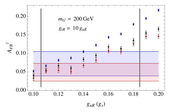
Figure 3: Contributions to the parton-level lab frame lepton asymmetry for a top non-universal axigluon with $m_{G^{\prime}}=200$ GeV and $g_{t_{R}}=10g_{u_{R}}$, for inclusive semi-leptonic $t\bar{t}$ events (blue), events passing semi-leptonic selection cuts after D0 Abazov et al. (2011) (black), and events passing selection cuts after CDF The CDF Collaboration (2012) (red). Error bars show Monte Carlo statistical error. One-sigma preferred regions are shown in blue for D0’s unfolded measurement (to be compared approximately to the inclusive events) and in red for CDF’s reconstruction-level measurement (to be compared to the events with CDF’s selection cuts) are shown in the shaded blue and red bands respectively. Vertical lines indicate the upper and lower boundaries of the globally preferred region of Fig. 11.

III.3 $t\bar{t}$ cross-section

The good agreement of the inclusive $t\bar{t}$ cross-section at both Tevatron and the LHC has been a major constraint on model building for the $A_{FB}^{t}$. Axigluons with purely axial couplings to light and top quarks contribute minimally to the total $t\bar{t}$ cross-section, but in the flavor-nonuniversal models we consider, at least one species of quark has non-vanishing vector couplings to the axigluon. The cross-section constraints are consequently tighter in these flavor-nonuniversal models.

In Fig. 4 we show contours corresponding to a 5% and 10% increase in the LO top pair production cross-section at the Tevatron for various choices of $g^{D}_{R}$ and $g^{t}_{R}$, in the down-type non-universal and top non-universal models. For our computation to be meaningful, the ratio of the top pair production cross-section at higher orders to the LO cross section should be similar in the SM and in the model with a light axigluon.

We choose $5\%$ as a benchmark because it is comparable to the combined error on the measurement, which is in agreement with the SM expectation. Note that the measured central values are above the predicted NNLO value for $m_{t}=173$ GeV CDF Collaboration (2009); Langenfeld et al. (2009), so a $5\%$ increase in the LO Tevatron top pair production cross-section is perfectly acceptable.

We superimpose on this figure the CDF $1\sigma$ preferred regions for the $A_{FB}^{t}$ (using only the inclusive unfolded measurement). As mass increases, the global maximum $A_{FB}^{t}$ decreases, leading to the sharp upward turn of the curves around $2m_{t}$. While the allowed contours around $2m_{t}$ appear open at larger couplings, eventually they will close (off the range of the plot), where $A_{FB}^{t}$ falls back below the measured value $-$ $1\sigma$ at sufficiently large coupling. Couplings large enough to provide a good fit to lower $A_{C}^{t}$ for the RH down-type non-universal model are marginally in agreement with the $t\bar{t}$ cross-section (see Fig. 1). RH top non-universal models are marginal only in the high mass range.

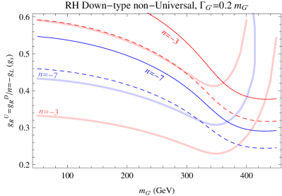
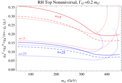
Figure 4: Contours corresponding to a 5% (dashed) and 10% (solid) increase in LO top pair production cross-section at the Tevatron. For reference, regions between the thick transparent lines of the same color indicate the CDF $A_{FB}^{t}$ 1$\sigma$ preferred regions. The $n=25$ region boundaries are drawn precisely only up to the strong coupling regime $g_{R}^{t}=25\times 0.2g_{s}$. Note that couplings large enough to provide a good fit to lower $A_{C}^{t}$ for the RH down-type non-universal model are marginally in agreement with the $t\bar{t}$ cross-section (See Fig. 1). RH top non-universal models have trouble only in the high mass range.

IV Direct searches at hadron colliders

Axigluons in the mass range of interest are light enough to have been copiously produced at past colliders. While in principle electron-positron colliders and electron-proton colliders can constrain axigluons, in practice the only existing constraints come from searches done at hadron colliders. In this section we discuss the most relevant constraints on axigluons, both broad and narrow, from various searches done at the SppS, the Tevatron, and the LHC.

IV.1 Narrow Resonances

Dijet resonances are constrained by experiments UA1 Albajar et al. (1988) and UA2 Alitti et al. (1993), dating from the time of the discovery of the $W$ and $Z$ bosons. At the SppS and also at the Tevatron, the relevant searches are those looking for single resonant production of a new state. For axigluons, single resonant production occurs through the coupling to quarks, and therefore the production cross-sections depend in detail on the flavor structure of the model.

Recent LHC searches by both ATLAS Aad et al. (2011); ATL (2012a) and CMS CMS (2012b) have looked for pairs of dijet resonances, which probe the QCD pair production of axigluons through their irreducible couplings to gluons, $gg\to G^{\prime}G^{\prime}$. Unitarity of the UV completion does not allow substantial suppression of the axigluon pair production cross-section below QCD strength: the tree-level non-covariant derivative coupling of the axigluon to gluons, $\chi$, is fixed by unitarity to the value $\chi=1$, and even large, order-one loop corrections to $\chi$ are not sufficient to reduce the pair production cross-section below experimental bounds. These searches exclude narrow axigluons in the entire mass range of interest, independent of the axigluon couplings to quarks. ATLAS searches exclude octet (pseudo-)scalars $\phi$ with masses in the range $100\;\mathrm{GeV}<m_{\phi}<287\;\mathrm{GeV}$. To understand how this limits axigluon pair production, it is necessary to translate the ATLAS limits on (pseudo-)scalars to (pseudo-)vectors. This is not entirely trivial, as the ATLAS searches use control regions to derive predictions for the background in the signal region, and scalars and vectors populate the signal and control regions differently. Fortunately for our purposes, vectors contribute proportionally much more to the background regions than the scalars do, and thus the limits on the cross-section derived for the scalar case are conservative when applied to vectors. We translate the ATLAS limits by taking into account the different efficiencies for scalars and vectors to pass the selection cuts, and show the resulting limits in Fig. 5. Pair production of narrow axigluons is comfortably excluded over the entire mass range considered by ATLAS, $100\;\mathrm{GeV}<m_{G^{\prime}}<350\;\mathrm{GeV}$. The exclusion is more stringent than the exclusion for scalars due to the significantly larger cross-sections for vectors Dobrescu et al. (2008). Note also that narrow axigluons cannot be “hidden” from the search and still remain narrow: suppressing the branching fraction to dijets by the $\mathcal{O}(0.1)$ factor necessary to satisfy the exclusions would then require axigluons to have a total width $\Gamma_{G^{\prime}}>0.1\,m_{G^{\prime}}$.

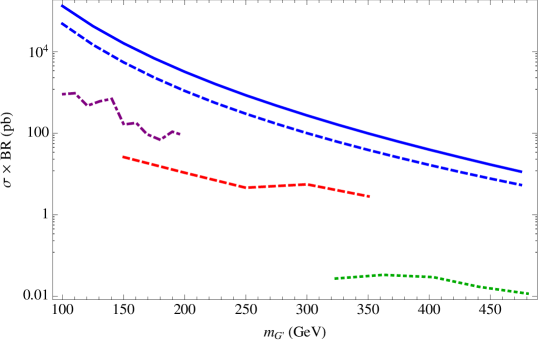
Figure 5: Rescaled ATLAS 95% CL and CMS 95% CL limits on the pair production of narrow axigluons. The red dashed line shows the ATLAS 5 fb^-1 limit ATL (2012a), the purple dash-dotted line the ATLAS 34 pb^-1 limit Aad et al. (2011), and the green dotted line the CMS 2.2 fb^-1 limit CMS (2012b). The leading order inclusive cross-section is shown by the blue solid line. To highlight the model independence of the exclusion we have also shown the LO pair production cross-section for $\chi=0$ in the blue dashed line.

Meanwhile, the search by CMS excludes octet vectors in the range $320\;\mathrm{GeV}<m_{G^{\prime}}<580\;\mathrm{GeV}$. Thus, the combination of ATLAS and CMS searches exclude narrow axigluons above 100 GeV in the entire mass range under consideration.

Very recently, a similar search for axigluon pair production at CDF, $q\bar{q}\to G^{\prime}G^{\prime}\to 4j$, has excluded the extremely low-mass region $50\;\mathrm{GeV}<m_{G^{\prime}}<125$ GeV, in the limit of vanishing quark coupling to axigluons CDF Collaboration . While application of this limit to axigluons which have the quark couplings necessary to explain $A_{FB}^{t}$ requires a careful treatment of quark-initiated contributions to the cross-section, the lack of any observed excess disfavors such axigluons below 100 GeV. Such extremely light, narrow axigluons can also be constrained by bounds on same-sign top production from the LHC Aguilar-Saavedra and Santiago (2012).

IV.2 Broad resonances

UA1 is the only collaboration to have used dijet searches to set limits on broad as well as narrow axigluons Albajar et al. (1988), conducting a dijet search for axigluons with width up to $\Gamma_{G^{\prime}}\lower 3.01385pt\hbox{$\;\stackrel{{\scriptstyle\textstyle<}}{{\sim}}\;$}0.4m_{G^{\prime}}$. This search covers the mass range above $m_{G^{\prime}}=150$ GeV, and excludes $g_{s}$-coupled axigluons up to $310$ GeV. Rescaling their limits, we obtain the constraints shown in Fig. 6, for both flavor-universal and down-type non-universal scenarios. We use Madgraph to obtain the relative fraction of down- and up-initiated events. Note that, in the majority of parameter space, the natural width into dijets is not sufficient to make the axigluon broad ($\Gamma\lower 3.01385pt\hbox{$\;\stackrel{{\scriptstyle\textstyle>}}{{\sim}}\;$}0.15m_{G}$), and in rescaling the limits we must therefore allow for non-zero branching fractions into undetected final states.

As a caveat, note that the UA1 study modeled the longitudinal and transverse momentum distributions of the $G^{\prime}$ using a sequential $Z^{\prime}$. The slight difference between the $G^{\prime}$ and $Z^{\prime}$ in the up versus down PDF support of the inclusive production cross-section does lead to a slight (percent level) change in efficiencies due to the different rapidity distributions of the center of mass. Of more concern is the difference in the transverse and longitudinal momentum distributions due to the different ISR spectra of a color octet versus a color singlet. However, as the cross-section UA1 used to set limits is leading order, the limits should be reliable.

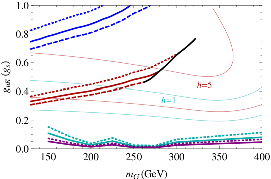
Figure 6: Topology-dependent CDF and UA1 95% CL limits on broad axigluons. CDF limits on $G^{\prime}\to 2X\to 4j$ are shown in cyan for flavor-universal axigluons and in purple for the scenario where $g_{u_{R}}=-g_{Q_{L}}=-g_{d_{R}}/5$, assuming in both cases $BR(G^{\prime}\to 4j)=1$. Solid lines assume that signal efficiencies are unchanged from the reference axigluon model in Ref. CDF Collaboration ; dotted lines incorporate a $50\%$ reduction in efficiency. The blue and red families of lines denote UA1 limits on $\sigma\times BR(G^{\prime}\to jj)$ for the flavor-universal case (blue), and the scenario where $g_{u_{R}}=-g_{Q_{L}}=-g_{d_{R}}/5$ (red). Here we have taken into account that in general $BR(G^{\prime}\to jj)<1$ in order to obtain a sufficiently large total width. The solid line applies to axigluons with a fixed total width $\Gamma_{tot}=0.2m_{G}$, the dotted line to a fixed total width $\Gamma_{tot}=0.3m_{G}$, and the dashed line to a fixed total width $\Gamma_{tot}=0.15m_{G}$. In black is the limit on the down-type non-universal axigluon with $BR(G^{\prime}\to jj)=1$, when the natural width lies in the range $0.15m<\Gamma_{G}<0.4m$. Regions above the lines are excluded. CDF one-sigma $A_{FB}^{t}$ preferred regions are shown for comparison.

Increasing the down-type coupling to alleviate tension with the CMS $A_{C}^{t}$ measurement tightens dijet constraints significantly, while a moderate increase in the top-quark coupling could allow for acceptably large values of $A_{FB}^{t}$ with couplings to light quarks small enough to evade dijet constraints.

The CDF paired dijet search CDF Collaboration can also constrain broad axigluons if they decay dominantly according to the cascade $G^{\prime}\to XX\to 4j$, and if the axigluon width is not substantially larger than the experimental resolution. We show limits from the CDF exclusion in Fig. 6. We have used the data for the case where the intermediate $X$ has mass $m_{X}=50$ GeV, but for fixed $m_{G^{\prime}}$ the cross-section limits do not depend strongly on $m_{X}$. In this search experimental resolutions on the four-jet invariant mass are on the order of $25\%$; larger axigluon widths will make it more difficult to obtain an accurate background estimate and fit a localized signal template. However, it can be seen from Fig. 6 that even after reducing the signal efficiency by $50\%$, axigluons decaying dominantly into dijets are eliminated as a possible explanation for $A_{FB}^{t}$.

IV.3 Constraints on daughter particles

To evade the LHC pair production exclusions, any light axigluon explanation for $A_{FB}^{t}$ must necessarily be either less than 100 GeV in mass Krnjaic (2012) or sufficiently broad, with sufficiently small branching fraction into dijets, to fail the selection cuts Tavares and Schmaltz (2011). In the window below 100 GeV, the tensions with PEW constraints we consider in the next section are important. Thus broad axigluons are the only states remaining that are obviously consistent with the data. In many regions of parameter space, however, the axigluon-SM couplings do not yield a large axigluon width ($\Gamma\lower 3.01385pt\hbox{$\;\stackrel{{\scriptstyle\textstyle>}}{{\sim}}\;$}0.1m_{G^{\prime}}$), necessitating the introduction of new colored degrees of freedom to provide a BSM decay mode for the axigluon. The nature of these new degrees of freedom is highly model dependent, but in many cases they may be easier to search for than the axigluon itself. For example, the paired dijet searches discussed in IV.1 exclude the possibility of axigluon decay into pairs of octet scalars for axigluons in the mass range $200\;\mathrm{GeV}<m_{G^{\prime}}<574\;\mathrm{GeV}$. CDF CDF Collaboration excludes triplet scalars decaying to dijets in the mass range between 50 GeV and 100 GeV. In addition to the paired dijet searches, both CDF Aaltonen et al. (2011b) and CMS Chatrchyan et al. (2011, 2012c) have conducted searches for three jet resonances, excluding octet fermions in the mass ranges from $70\;\mathrm{GeV}<m_{f}<145\;\mathrm{GeV}$ and $200\;\mathrm{GeV}<m<460\;\mathrm{GeV}$ respectively, thereby constraining the decays of axigluons involving three-jet resonances. Other possibilities, involving longer or less symmetric decay chains, are less constrained. A detailed discussion of decay scenarios in light axigluon models and relevant constraints is provided in Gross et al. (2012).

V Precision electroweak

The strongest precision electroweak constraints on $G^{\prime}q\bar{q}$ couplings arise from the one-loop corrections to the $Zq\bar{q}$ vertex. These corrections act uniformly to increase the effective $Zq\bar{q}$ couplings, leading to significant constraints from the hadronic $Z$ width and the hadronic $Z$ pole production cross-section, $\sigma_{\text{had}}$. The related real emission process, $Z\rightarrow G^{\prime}q\bar{q}$, is relevant when $m_{G^{\prime}}<m_{Z}$ and should also be taken into account. Contributions from $Zb\bar{b}$ observables and the $S$ and $T$ parameters are subdominant, as they are for heavy axigluons Haisch and Westhoff (2011).

We recomputed the one-loop corrections to the $Zq\bar{q}$ vertices and incorporated corrections for large axigluon widths. Broad widths tend to increase the contribution to the hadronic $Z$ width, particularly close to the $Z$ mass and below. In this region, a large axigluon width increases the contribution to the hadronic $Z$ width by (for example) about 5% at $m_{Z}$ for a 40% width. Much above the $Z$ mass, broad widths minimally affect PEW corrections. The contribution to the hadronic $Z$ width from real emission of axigluons below the $Z$ mass can be approximated from the expression in Carone and Murayama (1995). Further details on the inclusion of the width and the extraction of the real emission contribution can be found in Appendix B.1.

As in Haisch and Westhoff (2011), to derive constraints we use the combined LEP results on $\Gamma_{Z}$ and $\sigma_{\text{had}}$ assuming lepton universality Schael et al. (2006). We use the same SM inputs as Haisch and Westhoff (2011). The resulting $95\%$ C.L. exclusions for 0% and $20\%$ widths are plotted in Fig. 7. We show contours for couplings of the form $g_{R}^{D}=hg_{R}^{U}$. The $h=1$ contour corresponds to the flavor universal case as well as the top non-universal case since the top coupling does not enter the correction. Limits for masses below $m_{Z}$ should be considered cautiously in light of the fact that in this mass range the axigluon can affect the running of $\alpha_{s}$ and thus also the extraction of SM parameters used in the calculation of $\Gamma_{\text{had}}$. On the other hand, careful analysis of the running of $\alpha_{s}$ would provide yet another bound in this mass range. To estimate possible ambiguities associated with extracting $\alpha_{s}$ we include a curve assuming 1 % decrease in $\alpha_{s}$ for $m_{G^{\prime}}<m_{Z}$ in the summary plots of §VI (see Table 4 and Figs. 10-11).

The universal axigluon (top red line in Fig. 7) with couplings sufficient to reproduce the measured $A_{FB}^{t}$ is excluded below 100 GeV. PEW constraints rule out larger regions of parameter space as $h$ becomes more negative. For instance, models with $g^{D}_{R}\lesssim-5g^{U}_{R}$ appear to be in tension with PEW measurements for masses below about 200 GeV.

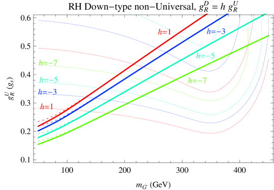
Figure 7: 95% C.L. exclusion contours from $\sigma_{\text{had}}$ and $\Gamma_{Z}$ measurements at LEP for axigluons with purely axial couplings to up-type quarks and modified couplings to down-type quarks of the form $g_{R}^{D}=hg_{R}^{U}$. Solid curves correspond to including a width $\Gamma_{G^{\prime}}/m_{G^{\prime}}=0.2$ (see Appendix B.1) and dotted curves (visible only at low mass) correspond to the zero width limit. As can be seen, the effect of the finite width is very small. An additional contribution from axigluon emission for masses below $m_{Z}$ is included; see the text for a discussion. For reference, the corresponding boundaries of the CDF $A_{FB}^{t}$ 1$\sigma$ preferred region (thin, curves of corresponding color) are shown.

As the PEW constraints are due to loop corrections, they can change depending on additional UV content in the model. It is therefore of interest to ask how the PEW constraints depend on the minimal UV completion of the phenomenological axigluon model. A UV-complete description of an axigluon with small ($<g_{s}$) axial couplings to quarks necessarily requires new heavy fermion degrees of freedom, as reviewed in Appendix A. Loops of heavy fermions, $Q_{h}$, and the axigluon can contribute to the vertex correction, as in Fig. 8. Once the axigluon mass and light quark couplings are fixed, the free parameters are the masses of the heavy fermions and the gauge mixing angle $\tan\theta$; the heavy fermion couplings to the axigluon and to the light quarks are otherwise determined. The new fermions, in particular, have been proposed as possible new decay modes for the axigluon Tavares and Schmaltz (2011); Gross et al. (2012), requiring at least one flavor to be light, and thus relevant for the PEW calculation.

Figure 8: Representative diagrams involving heavy vector-like quarks $Q_{h}$ (double lines) and scalar $\hat{\phi}$ (dashed lines) which contribute to the $Zq\bar{q}$ vertex correction.

We have computed the contribution from heavy fermions to the $Zq\bar{q}$ vertex correction and find that the sign of the contribution is the same as that of the correction from axigluon and light quarks alone. The PEW bounds from an axigluon alone are thus conservative. PEW bounds for a few representative choices of heavy quark mass (and flavor) are shown in Fig. 9. More details of the calculation can be found in the appendix §B.2.

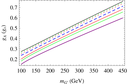
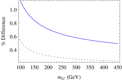
Figure 9: Left: 95% C.L. exclusion contours from $\sigma_{\text{had}}$ and $\Gamma_{Z}$ measurements at LEP for flavor-universal axigluons in the presence of no species (solid black, top), one species of heavy quark from the UV completion with coupling to $u_{R}$ (red dotted), $u_{L}$ (solid red), $d_{R}$ (green dotted—essentially on top of no species curve), $d_{L}$ (solid green), and to all four first-generation species $u_{R},u_{L},d_{R},d_{L}$ (purple). For these curves we take the new fermions to have mass $m_{Q_{h}}=m_{G^{\prime}}/2$. With this choice the contribution of the scalar is imperceptible on the plot, at least for scalar masses $m_{\hat{\phi}}\geq m_{Q_{h}}$; for smaller masses real emission would come into play. The blue dashed curve shows the exclusion contour given $m_{Q_{h}}=4m_{G^{\prime}}$ and heavy quarks coupling to $u_{R},u_{L},d_{R},d_{L}$, not including the scalar contribution. We have taken the coupling strength of the new fermion to standard model quark and axigluon to be double the axigluon-quark-quark coupling: $g_{\text{mix}}=2g_{A}$. See the appendix §B.2 for details. Right: Percent difference between constraint curves $g_{A}(m_{G^{\prime}})$ including and not including scalar contributions, in the presence of four heavy quarks from the UV completion coupling to $u_{R},u_{L},d_{R},d_{L}$, with $m_{Q_{h}}=m_{\hat{\phi}}=m_{G^{\prime}}/2$ (blue), and with $m_{Q_{h}}=4m_{G^{\prime}}$, $m_{\hat{\phi}}=m_{G^{\prime}}/2$ (dotted purple). Here again we choose $g_{\text{mix}}=2g_{A}$ for purposes of illustration.

Typical UV completions also contain a neutral scalar $\hat{\phi}$, the uneaten remnant of the field responsible for spontaneous symmetry breaking. Like the axigluon, this scalar also has off-diagonal $Q_{h}$-$q$ couplings with a fixed strength, and can contribute to PEW corrections via the right-hand diagram in Fig. 8. The calculation of this correction is also presented in §B.2. We find that it has the opposite sign as that from the axigluon-light quark loop and so therefore could serve to moderate precision electroweak corrections. On the other hand, the coupling entering the correction is related to that entering the heavy quark correction times the ratio of new heavy fermion to axigluon mass (see Eq. (B.36)). If new fermions are light enough to increase the axigluon widths, the scalar contribution is subdominant. This is shown in the right-hand panel of Fig. 9, where it can be seen that, while the scalar contribution does weaken the PEW constraint, it is a very mild effect in comparison to the effects of loops of fermions.

VI Results and Conclusions

We have examined constraints on light axigluon models for the Tevatron top forward-backward asymmetry from the LHC charge asymmetry, dijet and multijet searches, and precision electroweak observables. We considered only broad axigluons, as paired dijet resonance searches are devastating for narrow axigluons, regardless of the flavor structure.

Name:	Curve(s) plotted	Value fitted
CDF AFB:	$\pm 1\sigma$ band (solid dark blue), Aaltonen et al. (2012)	$0.164-0.066\pm 0.045\pm 0.020$
D0 AFB:	$\pm 1\sigma$ band (solid cyan), Abazov et al. (2011)	$0.196-0.063\pm 0.065\pm 0.019$
CMS AC:	$+1\sigma$ curve (solid purple), preferred region below, CMS Collaboration (2012)	$0.004-0.0115\pm 0.0156\pm 0.0006$
ATLAS AC:	$\pm 1\sigma$ band (solid green), ATL (2012b)	$0.029-0.006\pm 0.023\pm 0.002$
PEW:	LEP precision electroweak using $\sigma_{\text{had}}$ and $\gamma_{Z}$, 95% C.L. exclusion (solid black, dashed black for ${\delta\alpha_{s}\over\alpha_{s}}\sim-1\%$ below $m_{Z}$), Schael et al. (2006); Haisch and Westhoff (2011)	$\Gamma_{Z}^{\text{exp.}}=2.4952\pm 0.0023$ GeV,       $\sigma_{\text{had}}^{\text{exp.}}=41.540\pm 0.037$ nb, $\text{correlation}=\left(\begin{smallmatrix}1&-0.3\\ -0.3&1\end{smallmatrix}\right)$, $\Gamma_{Z}^{\text{SM}}=2.4945\pm 0.0007$ GeV,       $\sigma_{\text{had}}^{\text{SM}}=41.482\pm 0.006$ nb
Tevatron $\sigma$:	10% over LO SM $\sigma_{t\bar{t}}$ (reddish-pink, solid), off scale on most plots	$5.7\text{pb}\pm 10\%$
CDF high-mass AFB:	$\pm 1\sigma$ band (dashed dark blue), Aaltonen et al. (2012)	$0.295-0.1\pm 0.066\pm 0.03$
UA1 dijets (broad):	95% exclusion (solid brown), Albajar et al. (1988)

Table 4: Curves plotted in Figs. 10 and 11. References for experimental inputs are noted where relevant. For the charge asymmetry measurements “1$\sigma$” is taken to be the combined statistical $\oplus$ systematic experimental $\oplus$ Standard Model expectation error. Unless noted otherwise, the “Value fitted” is (experiment central value)$-$(SM prediction)$\pm$(experimental error)$\pm$(SM prediction error). For each curve, we take the Standard Model prediction and associated error as quoted by the collaboration, except we apply a correction for electroweak contributions to D0’s values. Following CDF, we multiply the SM NLO expectation by 1.26 and estimate a 30% error on the expectation.

Besides the Tevatron measurements, the most important constraints come from the LHC charge asymmetry and precision electroweak observables. The LHC charge asymmetry has the potential to severely constrain light axiglue models for $A_{FB}^{t}$, but the current spread in the central values measured by ATLAS and CMS leaves the situation unsettled. Future evolution towards the small values preferred by the current semileptonic measurement of CMS would be devastating for flavor-universal models. Precision electroweak constraints eliminate a significant corner of the very low-mass parameter space.

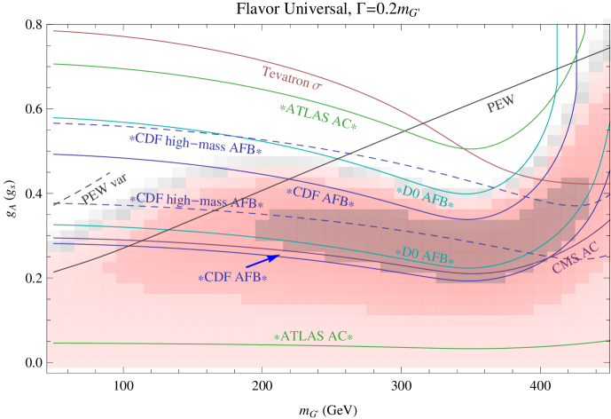
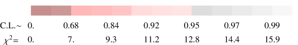
Figure 10: Summary of constraints on flavor-universal axigluons in the mass-coupling plane. Contours correspond to those listed in Table 4. We plot $1\sigma$ contours for asymmetry parameters and $95\%$ exclusion curves for precision electroweak (PEW); for the Tevatron cross-section, we use a 10% increase of LO $\sigma_{t\bar{t}}$ as a benchmark. The 95% C.L. UA1 broad dijet resonance search constraint is off the plot. Curve labels sit on the preferred side of the boundary, and curves that are part of a band on the plot are indicated by asterisks. Note that for axigluon masses in the $2m_{t}$ range, top asymmetries can attain a global maximum at moderate coupling strengths, which gives rise to a sharp upward turn of the asymmetry bands near $2m_{t}$. The bands close off of the plot. See the discussion in §III.3. The $\chi^{2}$ value computed using the first six measurements listed in the right-hand column of Table 4 is superimposed. (The correlation between $\sigma_{Z}$ and $\Gamma_{Z}$ is taken into account in the fit.)

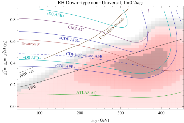
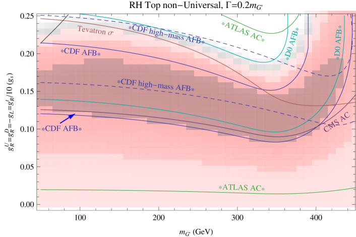
Figure 11: Summary of constraints for RH down-type non-universal axigluons with $g_{R}^{D}=-5g_{R}^{U}$ (top) and RH top non-universal axigluons with $g_{R}^{t}=10g_{R}^{U}$ (bottom). Contours correspond to those listed in Table 4; refer also to Fig. 10. Note that the RH down-type non-univeral model can simultaneously satisfy the CMS $A_{C}^{t}$ constraint and Tevatron $A_{FB}^{t}$ constraints (see also Fig. 1) at $1\sigma$, in contrast to the flavor-universal and RH top non-universal models.

We considered, in addition to flavor-universal axigluons, two flavor structures that can ameliorate either one of these constraints. Down-type nonuniversal models can ameliorate tension between LHC and Tevatron top asymmetries, but are significantly more constrained by PEW; top non-universal models can evade constraints from PEW, but do not help with the tension with the LHC $A_{C}^{t}$. In addition, top non-universal models are constrained by measurements of the lepton asymmetry at the Tevatron.

Our conclusions are shown in the plots Figs. 10 and 11, which show the parameter space consistent with all constraints at 1$\sigma$. The PEW constraints shown are $95\%$ C.L. and the Tevatron cross-section curve corresponds to a $10\%$ increase above the Standard Model in the leading order cross-section. The contours are superimposed on a granular density plot of a $\chi^{2}$ fit using the CDF and D0 measurements of the inclusive $A_{FB}^{t}$, the ATLAS and CMS $A_{C}^{t}$ measurements, and LEP’s combined measurement of $\sigma_{\text{had}}$ and $\Gamma_{Z}$. In all we used 6 inputs, with the only cross-correlation being between $\Gamma_{Z}$ and $\sigma_{\text{had}}$.

Note in particular that for the flavor-universal and top nonuniversal models, the globally preferred region lies outside the 1-sigma band preferred by the CMS $A_{C}^{t}$ measurement almost everywhere. This highlights the potential power of the LHC charge asymmetry measurements. Out of all the indirect constraints considered here, a reduction of a factor 2 in the error bars of the LHC charge asymmetry measurement will have the most impact in ruling out the remaining regions of parameter space. The down-type nonuniversal models which can be brought into agreement with the CMS asymmetry measurement encounter instead accentuated difficulty with PEW constraints.

Axigluons remain one of the best options for explaining the Tevatron forward-backward asymmetry with new physics. Much of the parameter space has been closed, in particular for narrow axigluons, and additional avenues should also be sought to explain the signal observed by Tevatron. While direct searches for broad axigluons are challenging and model dependent, we have shown that indirect observables are capable of tightly constraining admissible windows without reference to any specific decay scenario. Moreover, the combination of constraints from LHC charge asymmetries, PEW observables, and the lepton asymmetry leaves no obvious flavor avenue open to escape the tightening net of indirect constraints.

Acknowledgements: It is a pleasure to thank B. Dobrescu, M. Schmaltz, S. Westhoff, and D. Whiteson for useful conversations. JS thanks A. Falkowski and M. Schmaltz for collaboration on a related project. JS was supported by DOE grant DE-FG02-92ER40704, NSF grant PHY-1067976, and the LHC Theory Initiative under grant NSF-PHY-0969510. KZ is supported by NSF CAREER award PHY 1049896 as well by the DOE under grant de-sc0007859. JS and KZ thank the Aspen Center for Physics under grant NSF-PHY-1066293, as well as the Galileo Galilei Institute and the INFN, for hospitality and partial support during the completion of this work.

Appendix A Minimal UV Completions

In this section we review how to obtain axigluon models with small quark-axigluon couplings from a UV-complete description of spontaneous symmetry breakdown. We will neglect considerations of anomaly cancellation.

As discussed in section II, the minimal symmetry breaking structure that can realize a massive octet vector is $SU(3)_{1}\times SU(3)_{2}\to SU(3)_{c}$. Taking the breaking to be due to the vacuum expectation value of a bifundamental $\langle\phi\rangle=f\mathbbm{1}$ and denoting the coupling constants of the two groups as $g_{1}<g_{2}$, the strong coupling constant is, as usual,

$$g_{s}=\frac{g_{1}g_{2}}{\sqrt{g_{1}^{2}+g_{2}^{2}}}\equiv g_{1}\cos\theta,$$ (A.8)

while the axigluon, $G^{\prime}$, and SM gluon, $g$, are given by the following linear combination of UV gauge fields

$$G^{\prime\mu} = \sin\theta G_{1}^{\mu}-\cos\theta G_{2}^{\mu}$$ (A.9)

$$g^{\mu} = \cos\theta G_{1}^{\mu}+\sin\theta G_{2}^{\mu}.$$ (A.10)

The gluon remains massless, while the axigluon obtains a mass

$$m_{G^{\prime}}=\sqrt{g_{1}^{2}+g_{2}^{2}}f.$$ (A.11)

Quark-axigluon couplings depend on the embedding of the SM quarks in the group $SU(3)_{1}\times SU(3)_{2}$. First consider a (Weyl) quark $Q$ transforming as a fundamental under $SU(3)_{1}$. After spontaneous symmetry breakdown, its coupling to the axigluon is

$$\mathcal{L}_{q1}=g_{s}\tan\theta\,G^{\prime}_{\mu}\,Q^{{\dagger}}\bar{\sigma}^{\mu}Q.$$ (A.12)

Meanwhile, a quark $Q$ transforming as a fundamental under $SU(3)_{2}$ couples to the axigluon as

$$\mathcal{L}_{q2}=-g_{s}\cot\theta\,G^{\prime}_{\mu}\,Q^{{\dagger}}\bar{\sigma}^{\mu}Q.$$ (A.13)

Since if the left-handed fields couple to $SU(3)_{1}$, the right-handed fields must couple to $SU(3)_{2}$ (or vice-versa) in order to get axial couplings to $G^{\prime}$, we can thus see immediately that couplings of the left- and right-handed fields to the axigluon cannot both be smaller than $g_{s}$. It is therefore necessary to introduce heavy fermions that can mix with the SM quark fields and modify their axigluon couplings Dobrescu et al. (2008); Tavares and Schmaltz (2011); Cvetic et al. (2012).

For definiteness consider the case where $Q$ is a fundamental under $G_{1}$ and introduce $\hat{Q},\bar{Q}$ transforming as a fundamental and an anti-fundamental respectively under $G_{2}$, such that $\hat{Q}$ has the same $SU(2)_{L}\times U(1)_{Y}$ quantum numbers as $Q$, and $\bar{Q}$ has the same $SU(2)_{L}\times U(1)_{Y}$ quantum numbers as $Q^{\dagger}$. Then mixing can be obtained through the Lagrangian

$$\mathcal{L}_{mix}=\bar{Q}\left(M\hat{Q}+\lambda\phi Q\right)+\mbox{H.c.},$$ (A.14)

where $\phi$ is the field responsible for the spontaneous breakdown of $SU(3)_{1}\times SU(3)_{2}\to SU(3)_{c}$. When $\phi$ picks up its vev, $\phi=f+\sqrt{1/6}\,\hat{\phi}$, the resulting Lagrangian is

$$\mathcal{L}_{mix}=\sqrt{M^{2}+\lambda^{2}f^{2}}\,\bar{Q}Q_{h}+\frac{\lambda\cos\alpha}{\sqrt{6}}\,\hat{\phi}\bar{Q}q+\ldots+\mbox{H.c.},$$ (A.15)

where the mass eigenstates $Q_{h}$, $q$ are given by

$$Q_{h} = \cos\alpha\,\hat{Q}+\sin\alpha\,Q$$ (A.16)

$$q = -\sin\alpha\,\hat{Q}+\cos\alpha\,Q$$ (A.17)

in terms of the mixing angle

$$\cos\alpha=\frac{M}{\sqrt{M^{2}+\lambda^{2}f^{2}}}.$$ (A.18)

Note that

$$m_{Q_{h}}=\sqrt{M^{2}+\lambda^{2}f^{2}}.$$ (A.19)

The couplings of the different quark states to the two vector states can now be read off from the kinetic terms,

$$\frac{1}{g_{s}}\mathcal{L}_{axi} = Q_{h}^{\dagger}\bar{\sigma}^{\mu}Q_{h}\left(g_{\mu}+(-\cos^{2}\alpha\cot\theta+\sin^{2}\alpha\tan\theta)G_{\mu}\right)+$$

$$q^{\dagger}\bar{\sigma}^{\mu}q\left(g_{\mu}+(-\sin^{2}\alpha\cot\theta+\cos^{2}\alpha\tan\theta)G_{\mu}\right)+$$

$$\left(Q_{h}^{\dagger}\bar{\sigma}^{\mu}q+q^{\dagger}\bar{\sigma}^{\mu}Q_{h}\right)\left(\cos\alpha\sin\alpha(\cot\theta+\tan\theta)G_{\mu}\right).$$

The mixing angle $\cos\alpha$ is the necessary ingredient that allows us to freely dial the quark couplings to axigluons in the phenomenological low-energy Lagrangian. However, once $\cos\alpha$ (and $\cot\theta$) are fixed, so are the off-diagonal $q$-$Q$-$G^{\prime}$ couplings. This is particularly important for computing precision electroweak constraints, as we will discuss in the following section.

Appendix B Corrections to the $Z$-$q$-$\bar{q}$ vertex

B.1 One-loop corrections with finite axigluon width

In unitary gauge a convenient expression for the re-summed axigluon propagator is Baur and Zeppenfeld (1995)

$$D^{\mu\nu}_{G^{\prime}}(q) ={-i\over q^{2}-m_{G^{\prime}}^{2}+iq^{2}\gamma_{G^{\prime}}}\left(g^{\mu\nu}-{q^{\mu}q^{\nu}\over m_{G^{\prime}}^{2}}(1+i\gamma_{G^{\prime}})\right)$$ (B.21)

$$={1\over 1+i\gamma_{G^{\prime}}}{-i\over q^{2}-M_{G^{\prime}}^{2}}\left(g^{\mu\nu}-{q^{\mu}q^{\nu}\over M_{G^{\prime}}^{2}}\right)$$ (B.22)

where $\gamma_{G^{\prime}}=\Gamma_{G^{\prime}}/m_{G^{\prime}}$ and we have defined

$$M_{G^{\prime}}^{2}\equiv{m_{G^{\prime}}^{2}\over 1+i\gamma_{G^{\prime}}}.$$ (B.23)

Since all one-loop precision electroweak corrections of interest involve exactly one axigluon propagator, the finite width amplitude is thus related to the one-loop amplitude in the zero-width approximation, $\mathcal{M}_{0}(m_{G^{\prime}}^{2})$, via

$$\mathcal{M}(m_{G^{\prime}}^{2},\gamma_{G^{\prime}})={1\over 1+i\gamma_{G^{\prime}}}\mathcal{M}_{0}(M_{G^{\prime}}^{2}).$$ (B.24)

Since the Feynman prescription for handling poles is equivalent to assuming a small positive width, this prescription is consistent.

We calculated the one-loop correction to the $Zq\bar{q}$ vertex and fermion field strength corrections (in unitary gauge, assuming massless SM quarks in the loop) and find, in agreement with Haisch and Westhoff (2011), that in the zero-width limit the correction to the $Zq_{P}\bar{q}_{P}$ coupling, $f_{P}^{q}$, is

$$\delta f_{P}^{q}=f_{P}^{q}{{g_{P}^{q}}^{2}\over(4\pi)^{2}}c_{F}\,K(z)$$ (B.25)

where $z=m_{Z}^{2}/m_{G^{\prime}}^{2}$, $c_{F}={4\over 3}$, $g_{P}^{q}$ is the axigluon coupling to $q_{P}\bar{q}_{P}$ ($P=R$ or $L$), and $K(z)$ is given by

$$\mbox{Re}\,K(z) = -\frac{4+7z}{2z}+\frac{2+3z}{z}\ln z-\frac{2(1+z)^{2}}{z^{2}}\left(\ln z\ln(1+z)+\mbox{Li}_{2}(-z)\right),$$ (B.26)

$$\frac{1}{\pi}\mbox{Im}\,K(z) = -\frac{2+3z}{z}+\frac{2(1+z)^{2}}{z^{2}}\ln(1+z).$$ (B.27)

To include a finite width, multiply the above expression by $1/(1+i\gamma_{G^{\prime}})$ and let $m_{G^{\prime}}^{2}\rightarrow{m_{G^{\prime}}^{2}\over 1+i\gamma_{G^{\prime}}}$ as described above. The order ${{g_{P}^{q}}^{2}\over(4\pi)^{2}}$ correction to the $Z$ width then depends on the real part of this contribution:

$$\Gamma_{Z\rightarrow q\bar{q}}=n_{c}{G_{F}m_{Z}^{3}\over\pi 6\sqrt{2}}\bigg{(}r_{V}(q)(f_{R}^{q}+f_{L}^{q})^{2}\big{(}1+2{c_{F}\over(4\pi)^{2}}{f_{R}^{q}{g_{R}^{q}}^{2}+f_{L}^{q}{g_{L}^{q}}^{2}\over f_{R}^{q}+f_{L}^{q}}\text{Re}\left[{K(m_{Z}^{2}/M_{G^{\prime}}^{2})\over 1+i\gamma_{G^{\prime}}}\right]\big{)}\\ +r_{A}(q)(f_{R}^{q}-f_{L}^{q})^{2}\big{(}1+2{c_{F}\over(4\pi)^{2}}{f_{R}^{q}{g_{R}^{q}}^{2}-f_{L}^{q}{g_{L}^{q}}^{2}\over f_{R}^{q}-f_{L}^{q}}\text{Re}\left[{K(m_{Z}^{2}/M_{G^{\prime}}^{2})\over 1+i\gamma_{G^{\prime}}}\right]\big{)}\bigg{)}\\ +\Delta^{q}_{\text{EW/QCD}}$$ (B.28)

where $n_{c}=3$ and $r_{V}$ and $r_{A}$ are radiator factors that encode factorizable final state QED and QCD corrections and $\Delta^{q}_{\text{EW/QCD}}$ encodes non-factorizable corrections Haisch and Westhoff (2011).

For axigluon masses below $m_{Z}$, the $Z$ width is enhanced not only though the vertex correction but also through real emission of an axigluon, $Z\rightarrow q\bar{q}G^{\prime}$. The correction to the $Z$ width from vertex corrections and from real emission of a light vector boson coupling to baryon number was computed in Carone and Murayama (1995),

$$\left.\frac{\Delta\Gamma(Z\to\mbox{hadrons})}{\Gamma(Z\to q\bar{q})}\right|_{\mathrm{real}}=C\times(F_{1}(x)+F_{2}(x)),$$ (B.29)

where $C$ is a numerical constant, $F_{1}$ is the form factor due to real emission,

$$F_{1}(x) = (1+x)^{2}\left(3\ln x+(\ln x)^{2}\right)+5(1-x^{2})-2x\ln x$$

$$\phantom{move}-2(1+x)^{2}\left(\ln(1+x)\ln x+\mbox{Li}_{2}\left(\frac{1}{1+x}\right)-\mbox{Li}_{2}\left(\frac{x}{1+x}\right)\right)$$

with $x=m_{G}^{2}/m_{Z}^{2}=1/z$, and $F_{2}(x)=\text{Re}[K(1/x)]$ is the form factor due to the vertex correction, which we independently computed. For flavor-universal axigluons, in the limit as final state QED and QCD corrections are neglected, the constant in Eq. (B.29) becomes $C={2n_{f}c_{F}g_{A}^{2}\over(4\pi)^{2}}$ where $n_{f}=5$. Because of a nontrivial cancellation of IR divergences (the limit as $x\to 0$) in the sum $F_{1}(x)+F_{2}(x)$, in the $\gamma_{G^{\prime}}\rightarrow 0$ limit we can identify the form factor due to real emission of axigluons as $F_{1}$; we make the replacement $K(z)\rightarrow K(z)+F_{1}(1/z)$ in Eq. (B.28) to account for real emission when $m_{G^{\prime}}<m_{Z}$. For substantial nonzero axigluon widths, $\gamma_{G^{\prime}}>0$, making the replacement $K(z)\rightarrow K(z)+F_{1}(1/z)$ is an estimate. Because other issues such as the extraction of $\alpha_{s}$ arise for sub-$m_{Z}$ axigluon masses, the estimate is sufficient for our current purposes.

B.2 Heavy quark contributions

The off-diagonal $G^{\prime}$-$q$-$Q_{h}$ vertex is a necessary consequence of having quarks with phenomenogically acceptable axigluon couplings. While the magnitude of the coupling is fixed, the mass of the heavy quark is still a free parameter, so the minimal UV completion does not lead to a single sharp prediction for PEW calculations. In the decoupling limit, $m_{Q_{h}}\gg m_{G^{\prime}}$, the PEW calculation of the previous subsection provides a lower bound to the total contribution. Since the quark $Q_{h}$ has been proposed Tavares and Schmaltz (2011) as a possible additional decay mode to widen the axigluon, it is very interesting to consider the cases where $2m_{Q_{h}}<m_{G^{\prime}}$ and $m_{Q_{h}}<m_{G^{\prime}}$ (for a mixed $Q_{h}$-$q$ decay). Specifying $\theta$ and $m_{Q_{h}}$ then yields a unique prediction for each pair of values $(m_{G^{\prime}},g_{P})$.

The heavy quark contributions shift the effective $Zq_{P}\bar{q}_{P}$ coupling by an amount

$$\delta f_{P}^{q}=f_{P}^{q}{{g_{\text{mix}}}^{2}\over(4\pi)^{2}}c_{F}\,K_{h}(z_{Z},z_{Q_{h}})$$ (B.31)

where from Eq. A we have $g_{\text{mix}}=g_{s}\sin 2\alpha/\sin 2\theta$, $z_{Z}=m_{Z}^{2}/m_{G^{\prime}}^{2}$, $z_{Q_{h}}=m_{Q_{h}}^{2}/m_{G^{\prime}}^{2}$, and the form factor $K_{h}(z_{Z},z_{Q_{h}})$ is given by the following integral over Feynman parameters,

$$K_{h}(z_{Z},z_{Q_{h}})=\int_{0}^{1}\int_{0}^{1-x}f_{\text{1}}(x,y;z_{Z},z_{Q_{h}})\,dy\,dx+\int_{0}^{1}f_{\text{2}}(x;z_{Q_{h}})\,dx$$ (B.32)

where

$$f_{2}(x;z_{Q_{h}})=2-2x^{2}(1-z_{Q_{h}})+(1+3x^{2}(1-z_{Q_{h}})-x(4+z_{Q_{h}}))\log(1-x(1-z_{Q_{h}})).$$ (B.33)

and

$$f_{\text{1}}(x,y;z_{Z},z_{Q_{h}})=-\Delta_{\text{1}}+{((1-x)(1-y)z_{Z}+z_{Q_{h}})(2+xyz_{Z})\over\Delta_{1}}-(4-z_{Z}(x+y-2xy)+z_{Q_{h}})\\ +(4-z_{Z}-z_{Q_{h}}+3(x+y)(z_{Z}-2(1-z_{Q_{h}}))-12xyz_{Z})\log(\Delta_{1}),$$ (B.34)

with $\Delta_{\text{1}}=1-xyz_{Z}+(x+y)(z_{Q_{h}}-1)$.

In the limit as $m_{Q_{h}}\rightarrow 0$, $K_{h}$ reduces to $K$ in Eq. (B.25): $K_{h}(z_{Z},0)=K(z_{Z})$. In the limit as $m_{Q_{h}}\rightarrow\infty$, $K_{h}\rightarrow(7/36)m_{Z}^{2}/m_{G^{\prime}}^{2}$. Note that although $K_{h}$ is finite in the decoupling limit, the overall contribution of the heavy fermion still decouples, as the prefactor contains the coupling $g^{2}_{mix}$, which scales like $m_{Q_{h}}^{-2}$ as $m_{Q_{h}}\rightarrow\infty$ with $\lambda$ fixed. The ratios $\text{Re}[K_{h}\left(z_{Z},z_{Q_{h}}\right)]/\text{Re}[K(z_{Z})]$ and $\text{Im}[K_{h}\left(z_{Z},z_{Q_{h}}\right)]/\text{Im}[K(z_{Z})]$ are plotted in Fig. 12. Note that the sign of these contributions is the same as that of the contribution from the axigluon alone, and thus including these contributions to the $Z$ vertex correction will also act uniformly to increase the effective $Z$-$q$-$\bar{q}$ coupling. Therefore including heavy quarks as additional decay modes for the axigluon only increases the constraints from PEW observables.

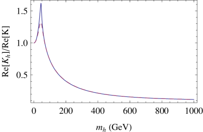
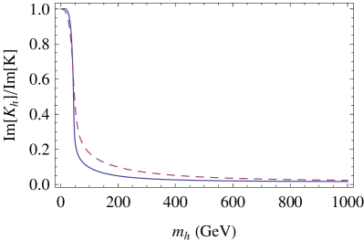
Figure 12: The ratios $\text{Re}[K_{h}\left(z_{Z},z_{Q_{h}}\right)]/\text{Re}[K(z_{Z})]$ and $\text{Im}[K_{h}\left(z_{Z},z_{Q_{h}}\right)]/\text{Im}[K(z_{Z})]$ are plotted for $z_{Z}={m_{Z}^{2}(1+i\gamma_{G^{\prime}})\over m_{G^{\prime}}^{2}(1+i\gamma_{Z})}$, $z_{Q_{h}}={m_{h}^{2}(1+i\gamma_{G^{\prime}})\over m_{G^{\prime}}^{2}(1+i\gamma_{h})}$, with $m_{Z}=91.2$ GeV, $\gamma_{Z}=2.50/91.2$, $m_{G^{\prime}}=250$ GeV, $\gamma_{G^{\prime}}=0.2$ and $\gamma_{h}=0.1$ (blue, solid) and $0.4$ (pink, dashed).

In general, there will also be contributions to the effective coupling from the uneaten part of the field that breaks $SU(3)_{1}\times SU(3)_{2}\to SU(3)_{c}$ via Eq. (A.15). The scalar-heavy-quark contributions shift the $Zq_{P}\bar{q}_{P}$ coupling by

$$\delta f_{P}^{q}=f_{P}^{q}{{\lambda^{2}\cos^{2}\alpha}\over 6(4\pi)^{2}}\,K_{\phi}\left({m_{Z}^{2}\over m_{\phi}^{2}},{m_{Q_{h}}^{2}\over m_{\phi}^{2}}\right).$$ (B.35)

Here,

$${\lambda^{2}\cos^{2}\alpha\over 6}=c_{F}g_{\text{mix}}^{2}{1\over 8}{m_{Q_{h}}^{2}\over m_{G^{\prime}}^{2}}$$ (B.36)

so for heavy quark masses less than $2\sqrt{2}/g_{s}$ times the axigluon mass, the coefficient entering the scalar-heavy quark correction is less than that entering the heavy quark-axigluon correction.

Let $z_{Z}={m_{Z}^{2}\over m_{\phi}^{2}}$ and $z_{Q_{h}}={m_{Q_{h}}^{2}\over m_{\phi}^{2}}$. The form factor $K_{\phi}$ is given by the following integral over Feynman parameters,

$$K_{\phi}(z_{Z},z_{Q_{h}})=\int_{0}^{1}\int_{0}^{1-x}f_{\text{3}}(x,y;z_{Z},z_{Q_{h}})\,dy\,dx+\int_{0}^{1}f_{\text{4}}(x;z_{Q_{h}})\,dx$$ (B.37)

where

$$f_{4}(x;z_{Q_{h}})=-x\log(x+z_{Q_{h}}(1-x))$$ (B.38)

and

$$f_{3}(x,y;z_{Z},z_{Q_{h}})=1-{xyz_{Z}+z_{Q_{h}}\over\Delta_{3}}+\log(\Delta_{3}),$$ (B.39)

with $\Delta_{3}=(x+y)z_{Q_{h}}+(1-x-y)-xyz_{Z}$.

We find the following limiting behavior of $K_{\phi}$:

$$K_{\phi}\longrightarrow\Bigg{\{}\begin{array}[]{c l}{1\over 3}{m_{Z}^{2}-3m_{Q_{h}}^{2}\over m_{\phi}^{2}}&\text{~{}~{}as~{}~{}}m_{\phi}\rightarrow\infty\\ -{7\over 36}{m_{Z}^{2}\over m_{Q_{h}}^{2}}&\text{~{}~{}as~{}~{}}m_{Q_{h}}\rightarrow\infty\\ f_{0}(m_{Z}^{2}/m_{\phi}^{2})&\text{~{}~{}as~{}~{}}m_{Q_{h}}\rightarrow 0\end{array}$$ (B.40)

where

$$f_{0}(x)={2\log x-1\over 4}+{1-\log x\over x}+{\log x\log(1+x)+\text{Li}_{2}(-x)\over x^{2}}-i\pi\left({\log(1+x)\over x^{2}}-{1\over x}+{1\over 2}\right).$$ (B.41)

We find that the scalar contribution has the opposite sign as the heavy quark-axigluon contribution, which could serve to moderate precision electroweak constraints for certain regions of parameter space. In Fig. 13 we plot $\text{Re}K_{\phi}$ and $\text{Im}K_{\phi}$ as a function of $m_{\phi}$ assuming $m_{Q_{h}}=125$ GeV (solid blue), 250 GeV (dashed pink), and 500 GeV (dotted yellow). By comparison, $\text{Re}K(m_{Z}^{2}/(250\text{GeV})^{2})=0.33$ and $\text{Re}K(m_{Z}^{2}/(100\text{GeV})^{2})=1.00$. In Fig. 14 we plot the real and imaginary contributions as functions of $m_{Q_{h}}$, with $m_{\phi}$ held fixed.

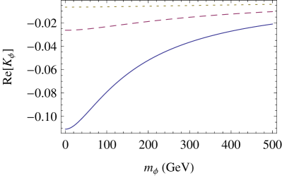
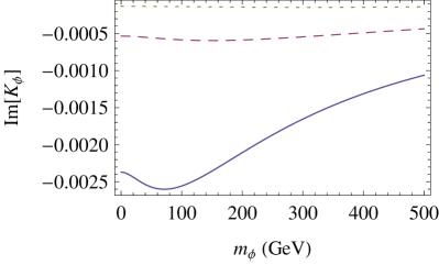
Figure 13: $\text{Re}[K_{\phi}\left(z_{Z},z_{Q_{h}}\right)]$ and $\text{Im}[K_{\phi}\left(z_{Z},z_{Q_{h}}\right)]$ are plotted for $z_{Z}={m_{Z}^{2}(1+i0.1)\over m_{\phi}^{2}(1+i0.03)}$, $z_{Q_{h}}={m_{Q_{h}}^{2}(1+i0.1)\over m_{\phi}^{2}(1+i0.05)}$, with $m_{Z}=91.2$ GeV, $m_{Q_{h}}=125$ GeV (solid blue), 250 GeV (dashed pink), and 500 GeV (dotted yellow).

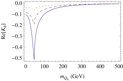
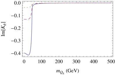
Figure 14: $\text{Re}[K_{\phi}\left(z_{Z},z_{Q_{h}}\right)]$ and $\text{Im}[K_{\phi}\left(z_{Z},z_{Q_{h}}\right)]$ are plotted for $z_{Z}={m_{Z}^{2}(1+i0.1)\over m_{\phi}^{2}(1+i0.03)}$, $z_{Q_{h}}={m_{Q_{h}}^{2}(1+i0.1)\over m_{\phi}^{2}(1+i0.05)}$, with $m_{Z}=91.2$ GeV, $m_{\phi}=125$ GeV (solid blue), 250 GeV (dashed pink), and 500 GeV (dotted yellow).

References

- Aaltonen et al. (2012) T. Aaltonen et al. (CDF Collaboration) (2012), eprint 1211.1003.
- Abazov et al. (2011) V. M. Abazov et al. (D0 Collaboration), Phys.Rev. D84, 112005 (2011), eprint 1107.4995.
- Aaltonen et al. (2011a) T. Aaltonen et al. (CDF Collaboration), Phys.Rev. D83, 112003 (2011a), eprint 1101.0034.
- Bernreuther and Si (2010) W. Bernreuther and Z.-G. Si, Nucl.Phys. B837, 90 (2010), eprint 1003.3926.
- Krohn et al. (2011) D. Krohn, T. Liu, J. Shelton, and L.-T. Wang, Phys.Rev. D84, 074034 (2011), eprint 1105.3743.
- Abazov et al. (2012) V. M. Abazov et al. (D0 Collaboration) (2012), eprint 1207.0364.
- The CDF Collaboration (2012) The CDF Collaboration, CDF Note 10807 (2012).
- Frampton et al. (2010) P. H. Frampton, J. Shu, and K. Wang, Phys.Lett. B683, 294 (2010), eprint 0911.2955.
- Chivukula et al. (2010) R. S. Chivukula, E. H. Simmons, and C.-P. Yuan, Phys.Rev. D82, 094009 (2010), eprint 1007.0260.
- Bai et al. (2011) Y. Bai, J. L. Hewett, J. Kaplan, and T. G. Rizzo, JHEP 1103, 003 (2011), eprint 1101.5203.
- Haisch and Westhoff (2011) U. Haisch and S. Westhoff, JHEP 1108, 088 (2011), eprint 1106.0529.
- Gresham et al. (2011a) M. I. Gresham, I.-W. Kim, and K. M. Zurek, Phys.Rev. D83, 114027 (2011a), eprint 1103.3501.
- Barcelo et al. (2012) R. Barcelo, A. Carmona, M. Masip, and J. Santiago, Phys.Lett. B707, 88 (2012), eprint 1106.4054.
- Alvarez et al. (2011) E. Alvarez, L. Da Rold, J. I. S. Vietto, and A. Szynkman, JHEP 1109, 007 (2011), eprint 1107.1473.
- Jung et al. (2010) S. Jung, H. Murayama, A. Pierce, and J. D. Wells, Phys.Rev. D81, 015004 (2010), eprint 0907.4112.
- Shu et al. (2010) J. Shu, T. M. Tait, and K. Wang, Phys.Rev. D81, 034012 (2010), eprint 0911.3237.
- Gresham et al. (2011b) M. I. Gresham, I.-W. Kim, and K. M. Zurek, Phys.Rev. D84, 034025 (2011b), eprint 1102.0018.
- Shelton and Zurek (2011) J. Shelton and K. M. Zurek, Phys.Rev. D83, 091701 (2011), eprint 1101.5392.
- Jung et al. (2011a) S. Jung, A. Pierce, and J. D. Wells, Phys.Rev. D83, 114039 (2011a), eprint 1103.4835.
- Jung et al. (2011b) S. Jung, A. Pierce, and J. D. Wells, Phys.Rev. D84, 091502 (2011b), eprint 1108.1802.
- Gresham et al. (2012a) M. I. Gresham, I.-W. Kim, and K. M. Zurek, Phys.Rev. D85, 014022 (2012a), eprint 1107.4364.
- Delaunay et al. (2011) C. Delaunay, O. Gedalia, Y. Hochberg, G. Perez, and Y. Soreq, JHEP 1108, 031 (2011), eprint 1103.2297.
- Aguilar-Saavedra and Perez-Victoria (2011a) J. Aguilar-Saavedra and M. Perez-Victoria, JHEP 1105, 034 (2011a), eprint 1103.2765.
- Craig et al. (2011) N. Craig, C. Kilic, and M. J. Strassler, Phys.Rev. D84, 035012 (2011), eprint 1103.2127.
- Knapen et al. (2012) S. Knapen, Y. Zhao, and M. J. Strassler, Phys.Rev. D86, 014013 (2012), eprint 1111.5857.
- Chatrchyan et al. (2012a) S. Chatrchyan et al. (CMS Collaboration) (2012a), eprint 1206.3921.
- ATLAS (2012) ATLAS, ATLAS-CONF-2012-096 (2012).
- Alvarez and Leskow (2012) E. Alvarez and E. C. Leskow, Phys.Rev. D86, 114034 (2012), eprint 1209.4354.
- Drobnak et al. (2012a) J. Drobnak, A. L. Kagan, J. F. Kamenik, G. Perez, and J. Zupan, Phys.Rev. D86, 094040 (2012a), eprint 1209.4872.
- Gresham et al. (2012b) M. I. Gresham, I.-W. Kim, S. Tulin, and K. M. Zurek (2012b), eprint 1203.1320.
- Aad et al. (2012) G. Aad et al. (ATLAS Collaboration) (2012), eprint 1203.4211.
- Chatrchyan et al. (2012b) S. Chatrchyan et al. (CMS Collaboration), Phys.Lett. B717, 129 (2012b), eprint 1207.0065.
- Fajfer et al. (2012) S. Fajfer, J. F. Kamenik, and B. Melic, JHEP 1208, 114 (2012), eprint 1205.0264.
- Delaunay et al. (2012) C. Delaunay, O. Gedalia, Y. Hochberg, and Y. Soreq (2012), eprint 1207.0740.
- Tavares and Schmaltz (2011) G. M. Tavares and M. Schmaltz, Phys.Rev. D84, 054008 (2011), eprint 1107.0978.
- Aguilar-Saavedra and Perez-Victoria (2011b) J. Aguilar-Saavedra and M. Perez-Victoria, Phys.Lett. B705, 228 (2011b), eprint 1107.2120.
- Krnjaic (2012) G. Z. Krnjaic, Phys.Rev. D85, 014030 (2012), eprint 1109.0648.
- Drobnak et al. (2012b) J. Drobnak, J. F. Kamenik, and J. Zupan, Phys.Rev. D86, 054022 (2012b), eprint 1205.4721.
- Kaplan and Schwartz (2008) D. E. Kaplan and M. D. Schwartz, Phys.Rev.Lett. 101, 022002 (2008), eprint 0804.2477.
- Gross et al. (2012) C. Gross, G. M. Tavares, C. Spethmann, and M. Schmaltz (2012), eprint 1209.6375.
- Cvetic et al. (2012) M. Cvetic, J. Halverson, and P. Langacker (2012), eprint 1209.2741.
- Grinstein et al. (2011a) B. Grinstein, A. L. Kagan, M. Trott, and J. Zupan, Phys.Rev.Lett. 107, 012002 (2011a), eprint 1102.3374.
- Grinstein et al. (2011b) B. Grinstein, A. L. Kagan, J. Zupan, and M. Trott, JHEP 1110, 072 (2011b), eprint 1108.4027.
- Aguilar-Saavedra and Juste (2012) J. Aguilar-Saavedra and A. Juste (2012), eprint 1205.1898.
- Kamenik et al. (2011) J. F. Kamenik, J. Shu, and J. Zupan (2011), eprint 1107.5257.
- CMS (2012a) Tech. Rep. CMS-PAS-TOP-12-010, CERN, Geneva (2012a).
- Manohar and Trott (2012) A. V. Manohar and M. Trott, Phys.Lett. B711, 313 (2012), eprint 1201.3926.
- Bernreuther and Si (2012) W. Bernreuther and Z.-G. Si, Phys.Rev. D86, 034026 (2012), eprint 1205.6580.
- Falkowski et al. (2011) A. Falkowski, G. Perez, and M. Schmaltz (2011), eprint 1110.3796.
- CDF Collaboration (2009) CDF Collaboration (2009), CDF note 9913.
- Langenfeld et al. (2009) U. Langenfeld, S. Moch, and P. Uwer, Phys.Rev. D80, 054009 (2009), eprint 0906.5273.
- Albajar et al. (1988) C. Albajar et al. (UA1 Collaboration), Phys.Lett. B209, 127 (1988).
- Alitti et al. (1993) J. Alitti et al. (UA2 Collaboration), Nucl.Phys. B400, 3 (1993).
- Aad et al. (2011) G. Aad et al. (ATLAS Collaboration), Eur.Phys.J. C71, 1828 (2011), eprint 1110.2693.
- ATL (2012a) Tech. Rep. ATLAS-CONF-2012-110, CERN, Geneva (2012a).
- CMS (2012b) Tech. Rep. PAS-EXO-11-016 (2012b).
- Dobrescu et al. (2008) B. A. Dobrescu, K. Kong, and R. Mahbubani, Phys.Lett. B670, 119 (2008), eprint 0709.2378.
- (58) CDF Collaboration, http://www-cdf.fnal.gov/danielw/fourjet/fourjet.html, CDF note NNNN.
- Aguilar-Saavedra and Santiago (2012) J. Aguilar-Saavedra and J. Santiago, Phys.Rev. D85, 034021 (2012), eprint 1112.3778.
- Aaltonen et al. (2011b) T. Aaltonen et al. (CDF Collaboration), Phys.Rev.Lett. 107, 042001 (2011b), eprint 1105.2815.
- Chatrchyan et al. (2011) S. Chatrchyan et al. (CMS Collaboration), Phys.Rev.Lett. 107, 101801 (2011), eprint 1107.3084.
- Chatrchyan et al. (2012c) S. Chatrchyan et al. (CMS Collaboration) (2012c), eprint 1208.2931.
- Carone and Murayama (1995) C. D. Carone and H. Murayama, Phys.Rev.Lett. 74, 3122 (1995), eprint hep-ph/9411256.
- Schael et al. (2006) S. Schael et al. (ALEPH Collaboration, DELPHI Collaboration, L3 Collaboration, OPAL Collaboration, SLD Collaboration, LEP Electroweak Working Group, SLD Electroweak Group, SLD Heavy Flavour Group), Phys.Rept. 427, 257 (2006), eprint hep-ex/0509008.
- CMS Collaboration (2012) CMS Collaboration (2012), CMS-PAS-TOP-11-030.
- ATL (2012b) Tech. Rep. ATLAS-CONF-2012-057, CERN, Geneva (2012b).
- Baur and Zeppenfeld (1995) U. Baur and D. Zeppenfeld, Phys.Rev.Lett. 75, 1002 (1995), eprint hep-ph/9503344.