Counting generalized Jenkins–Strebel differentials
Abstract.
We study the combinatorial geometry of “lattice” Jenkins–Strebel differentials with simple zeroes and simple poles on and of the corresponding counting functions. Developing the results of M. Kontsevich [K92] we evaluate the leading term of the symmetric polynomial counting the number of such “lattice” Jenkins–Strebel differentials having all zeroes on a single singular layer. This allows us to express the number of general “lattice” Jenkins–Strebel differentials as an appropriate weighted sum over decorated trees.
The problem of counting Jenkins–Strebel differentials is equivalent to the problem of counting pillowcase covers, which serve as integer points in appropriate local coordinates on strata of moduli spaces of meromorphic quadratic differentials. This allows us to relate our counting problem to calculations of volumes of these strata . A very explicit expression for the volume of any stratum of meromorphic quadratic differentials recently obtained by the authors [AEZ] leads to an interesting combinatorial identity for our sums over trees.
1. Introduction
1.1. Counting pillowcase covers
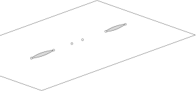
A geometric approach to volume computation for the strata in the moduli spaces of Abelian or quadratic differentials consists in counting square-tiled surfaces or pillowcase covers, see [EO01], [EO03], [EOP], [Z00]. A pillowcase cover is a ramified cover over branched over four points. Define a flat metric on such that the resulting pillowcase orbifold as in Figure 1

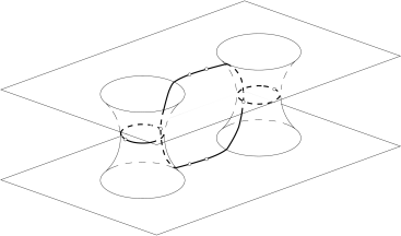
is glued from two squares of size . Choosing the four corners of the pillowcase as the four ramification points, we get an induced square tiling of the pillowcase cover, see Figure 2.
The flat structure on the pillowcase corresponds to the meromorphic quadratic differential on , where . The quadratic differential has four simple poles at the corners of the pillow and no other singularities. We shall see that the induced quadratic differential on defines an integer point (in appropriate local coordinates) in the ambient stratum of meromorphic quadratic differentials.
In this paper we want to count the number of nonisomorphic connected pillowcase covers of degree at most having the following ramification pattern. All ramification points are located over the corners of the pillowcase. All preimages of the corners are ramification points of degree two with exception for ramification points of degree three and for unramified points. For example, the pillowcase cover in Figure 2 has ramification points of degree three and unramified points. We do not specify how the projections of distinguished points are distributed between the four corners of the pillowcase .
Our restriction on the ramification data implies that the quadratic differential has exactly simple zeroes (located at the ramification points of degree three); it has exactly simple poles (located at nonramified preimages of the corners), and it has no other zeroes or poles. In particular, the pillowcase cover has genus zero.
In order to count pillowcase covers we note that if is a pillowcase cover, it can be decomposed into horizontal cylinders with integer widths, with zeros and poles lying on the boundaries of these cylinders, see Figure 2. We call these boundaries singular layers. Each singular layer defines a connected graph with a certain number of trivalent vertices, a certain number of univalent vertices, and with no vertices of any other valence. Actually, it is more convenient to consider the singular layer as a ribbon graph by taking a small tubular neighborhood of the singular layer inside the surface. The graph is metric: all edges have certain lengths measured by means of the flat structure. Since the length of the sides of each square of the tiling of the pillowcase cover is , and the vertices of each singular layer are located at the vertices of the squares, the lengths of all edges of our graph are half-integer. Note that the number of cylinders adjacent to a layer is expressed in terms of the number of zeroes and the number of poles on the corresponding layer as . Thus, by topological reasons is necessarily a nonnegative even number.
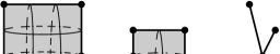
Developing the techniques of M. Kontsevich from [K92], we find a formula for the following counting function. Given positive integer numbers we count the number of ways to join cylinders of widths together by means of a connected half-integer ribbon graph having trivalent and univalent vertices; see Figure 3.
Theorem 1.1.
Let and be nonnegative integer numbers not equal simultaneously to zero such that is a nonnegative even number. Let , where , be the number of ways to attach cylinders of integer widths to all possible layers containing zeroes and poles, in such way that all edges of the resulting graph are half-integer. Up to the lower order terms one has
| (1.1) |
Theorem 1.1 is of independent interest; it is is proved in §3.5. To elaborate certain geometric intuition helpful in manipulating geometric counting functions we compute in §3.2 by hands the function corresponding to ribbon graphs from Figure 3.
Having studied the enumerative geometry of singular layers let us return to global pillowcase covers. Suppose there are cylinders of width and height respectively. Since the flat surface is a topological sphere, there are singular layers in the decomposition of . The total number of pillowcase covers of degree with this type of decomposition can be written as
| (1.2) |
where is a function counting the number of ways the cylinders of width can be glued at the layer , and . The factor arises from the possibility of twisting each cylinder around the waist curve; see §3.2 for more details.
Representing each singular layer by a vertex of an associated graph as in Figure 2, and every cylinder by an edge of such graph, we encode the decomposition of into cylinders by a global graph . We also record the information on the number of zeroes and the number of simple poles located at each layer . This extra structure is referred to as a decoration. Since is a topological sphere, the graph is a tree. Taking an appropriate sum of expressions (1.2) over all decorated trees we get the leading term of the asymptotics for the number of pillowcase covers (see §3.6 and Theorem 3.10 for exact statements).
On the other hand, we have the following recent result from [AEZ]:
Theorem.
It implies the main combinatorial identity stated in Theorem 3.10.
The formula for the volume (and, actually, a much more general formula for the volume of any stratum of meromorphic quadratic differentials with at most simple poles) is obtained in [AEZ] in a very indirect way through the analytic Riemann-Roch theorem, asymptotics of the determinant of the Laplacian of the singular flat metric, principal boundary of the moduli spaces, Siegel–Veech constants, and Lyapunov exponents of the Hodge bundle. The current paper develops a transparent geometric approach. We have to admit that from purely pragmatic point of view this natural geometric approach is, however, less efficient.
The situation with counting volumes of strata of Abelian differentials is somehow similar: the problem was solved by A. Eskin and A. Okounkov in [EO01] using methods of representation theory of the symmetric group, and developed further in [EO03] and in [EOP] using techniques of quasimodular forms. A straightforward counting of square-tiled surfaces works only for strata of small dimension, and becomes disastrously complicated when the dimension grows, see [Z00]. However, the technique elaborated in this naive geometric approach to the study of square-tiled surfaces, and the ties to various related subjects proved to be extremely helpful. For example, the separatrix diagrams (analogs of ribbon graphs representing singular layers) were used as one of the main instruments in classification [KZ00] of connected components of the strata. Multiple zeta values which appear in counting square-tiled surfaces represented by certain groups of separatrix diagrams, seem to have interesting applications to representation theory.
We believe that an ample description of the enumerative geometry of pillowcase covers combining direct geometric approach elaborated in the current paper, and the implicit analytic approach from [AEZ] could be helpful for various applications.
1.2. Reader’s guide
In §2 we present the basic background material on the natural volume element the moduli spaces of quadratic differentials. Namely, in §2.1 we introduce the canonical cohomological coordinates in each stratum of meromorphic quadratic differentials with at most simple poles. In §2.2 we define a canonical lattice in these coordinates which determines the natural linear volume element in the stratum. In §2.3 we show how volume calculation is related to counting of lattice points.
The original part of the paper is presented in §3. In §3.1 we show why lattice points in the stratum are represented by pillowcase covers which, in view of §2.3, explains why the volume calculation is equivalent to counting the pillowcase covers. In §3.2 we discuss in more details the functions from Theorem 1.1, study their elementary properties and prove formula (1.2). We consider in §3.2 a particular case corresponding to Figure 3 as an example, for which we perform an explicit by hand computation. In §3.4 we obtain a general expression for as a corollary from Kontsevich’s Theorem [K92]. We use this expression as a base of recurrence developed in §3.5, where we express in terms of . This recurrence allows us to prove in §3.5 Theorem 1.1. Finally, in §3.6 we compute the sum over all decorated trees and prove the main identity stated in Theorem 3.10. We illustrate this Theorem performing a detailed computation for the strata and in §3.7 and in §3.8 respectively.
Acknowledgments. The authors are happy to thank IHES, IMJ, IUF, MPIM, and the Universities of Chicago, of Illinois at Urbana-Champaign, of Rennes 1, and of Paris 7 for hospitality during the preparation of this paper. We thank the anonymous referee for their careful reading of the paper and helpful suggestions.
2. Canonical volume element in the moduli space of quadratic differentials
2.1. Coordinates in a stratum of quadratic differentials.
Consider a meromorphic quadratic differential having zeroes of arbitrary multiplicities but only simple poles on . Let be its singular points (zeros and simple poles). Consider the minimal branched double covering such that the induced quadratic differential on the hyperelliptic surface is already a square of an Abelian differential .
The zeros of the resulting Abelian differential correspond to the zeros of in the following way: every zero of of odd order is a ramification point of the covering, so it produces a single zero of ; every zero of of even order is a regular point of the covering, so it produces two zeros of . Every simple pole of defines a branching point of the covering; this point is a regular point of .
Consider the subspace of the relative homology of the cover with respect to the collection of zeroes of which is antiinvariant with respect to the induced action of the hyperelliptic involution. We are going to construct a basis in this subspace (in complete analogy with a usual basis of absolute cycles for a hyperelliptic surface).
We can always enumerate the singular points of in such a way that is a simple pole. Chose now a simple oriented broken line on joining consecutively all the singular points of except the last one. For every arc of this broken line, , the difference of their two preimages defines a relative cycle in . By construction such a cycle is antiinvariant with respect to the hyperelliptic involution. It is immediate to see that the resulting collection of cycles forms a basis in .
Note that, a preimage of a simple pole does not belong to the set . Thus, a preimage of an arc having a simple pole as one of the endpoints does not define a cycle in . However, since a simple pole is always a branching point, the difference of the preimages of such arc is already a well-defined relative cycle in .
Let be the ambient stratum for the meromorphic quadratic differential . The subspace in the relative cohomology antiinvariant with respect to the natural involution defines local coordinates in the stratum.
2.2. Normalization of the volume element.
For any flat surface in any stratum we have a canonical ramified double cover such that the induced quadratic differential on the Riemann surface is a global square of a holomorphic Abelian differential. We have seen in §2.1 that the subspace antiinvariant with respect to the induced action of the hyperelliptic involution on relative cohomology provides local coordinates in the corresponding stratum of quadratic differentials. We define a lattice in as the subset of those linear forms which take values in on .
We define the volume element on as the linear volume element in the vector space normalized in such way that the fundamental domain of the above lattice has volume .
We warn the reader that for this lattice is a proper sublattice of index of the lattice
Indeed, if a flat surface defines a lattice point for our choice of the lattice, then the holonomy vector along a saddle connection joining distinct singularities might be half-integer. (However, the holonomy vector along any closed saddle connection is still always integer.)
The choice of one or another lattice is a matter of convention. Our choice makes formulae relating enumeration of pillowcase covers to volumes simpler; see § 3. Another advantage of our choice is that the volumes of the strata and of the hyperelliptic components of the corresponding strata of Abelian differentials are the same (up to the factors responsible for the numbering of zeroes and of simple poles).
Convention 2.1.
Similar to the case of Abelian differentials we choose a real hypersurface in the stratum of flat surfaces of fixed area. We abuse notation by denoting by the space of flat surfaces of area (so that the canonical double cover has area ).
The volume element in the embodying space induces naturally a volume element on the hypersurface in the following way. There is a natural -action on : having we associate to the flat surface the flat surface
| (2.1) |
In particular, we can represent any as , where , and where belongs to the “hyperboloid”: . Geometrically this means that the metric on is obtained from the metric on by rescaling with linear coefficient . In particular, vectors associated to saddle connections on are multiplied by to give vectors associated to corresponding saddle connections on . It means also that , since . We define the volume element on the “hyperboloid” by disintegration of the volume element on :
| (2.2) |
where
Using this volume element we define the total volume of the stratum :
| (2.3) |
For a subset we let denote the “cone” based on :
| (2.4) |
Our definition of the volume element on is consistent with the following normalization:
| (2.5) |
where is the total volume of the “cone” measured by means of the volume element on defined above.
2.3. Reduction of volume calculation to counting lattice points
The volume of a stratum is defined by (2.5) as
where is the total volume of the “cone” measured by means of the volume element on defined in §2.2. The total volume of the cone is the limit of the appropriately normalized Riemann sums.
The volume element is defined as a linear volume element in cohomological coordinates, normalized by certain specific lattice. Chose a positive such that is integer, and consider a sublattice of the initial lattice of index partitioning every side of the initial lattice into pieces. The corresponding Riemann sums count the number of points of the sublattices which get inside the cone. Thus, by definition of the measure we get
We assume that is integer. Note that a flat surface represents a point of the -lattice, if and only if the surface (in the sense of definition (2.1)) represents a point of the integer lattice. Denoting by the set of flat surfaces in the stratum of area at most , and taking into consideration that
we can rewrite the above relation as
| (2.6) |
3. Counting generalized Jenkins–Strebel differentials
In this section we pass to counting the pillowcase covers. We have seen in §2.3 that volume calculation is equivalent to counting the lattice points. In §3.1 we discuss in more details the pillowcase covers and show that counting of lattice points is equivalent to the counting problem for pillowcase covers. Starting from section §3.2 we work exclusively with the strata .
In §3.2 we discuss in more details the functions from Theorem 1.1, study their elementary properties and prove formula (1.2). We consider in §3.2 a particular case corresponding to Figure 3 as an example, for which we perform an explicit (by hand) computation. In §3.4 we obtain a general expression for as a corollary from a theorem of Kontsevich [K92]. We use this expression as a base of recursion developed in §3.5, where we express in terms of . This recurrence relation allows us to prove in §3.5 Theorem 1.1. Finally, in §3.6 we compute the sum over all decorated trees and prove the main identity stated in Theorem 3.10. In §3.7 and §3.8 we illustrate our formula for concrete examples of the strata and correspondingly.
3.1. Lattice points, square-tiled surfaces, and pillowcase covers
Let be a lattice, and let be the associated torus. The quotient
by the map is known as the pillowcase orbifold. It is a sphere with four -orbifold points (the corners of the pillowcase). The quadratic differential on descends to a quadratic differential on . Viewed as a quadratic differential on the Riemann sphere, has simple poles at corner points. When the lattice is the standard integer lattice , the flat torus is obtained by isometrically identifying the opposite sides of a unit square, and the pillowcase is obtained by isometrically identifying two squares with the side by the boundary, see Figure 1.
Consider a connected ramified cover over of degree having ramification points only over the corners of the pillowcase. Clearly, is tiled by squares of the size in such way that the squares do not superpose and the vertices are glued to the vertices. Coloring the two squares of the pillowcase one in black and the other in white, we get a chessboard coloring of the square tiling of the the cover : the white squares are always glued to the black ones and vice versa.
Lemma 3.1.
Let be a flat surface in the stratum . The following properties are equivalent:
-
(1)
The surface represents a lattice point in ;
-
(2)
is a cover over ramified only over the corners of the pillow;
-
(3)
is tiled by black and white squares respecting the chessboard coloring.
Proof.
We have just proved that (2) implies (3). To prove that (1) implies (2) we define the following map from to . Fix a zero or a pole on . For any consider a path joining to having no self-intersections and having no zeroes or poles inside. The restriction of the quadratic differential to such admits a well-defined square root , which is a holomorphic form on the interior of . Define
Of course, the path is not uniquely defined. However, since the flat surface represents a lattice point (see the definition in §2.2), the difference of the integrals of over any two such paths and belongs to , so taking the quotient over the integer lattice and over we get a well-defined map. By definition of the pillowcase we have, . Thus, we have defined a map . It follows from the definition of the map, that it is a ramified cover, and that all regular points of the flat surface are regular points of the cover. Thus, all ramification points are located over the corners of the pillowcase.
A similar consideration shows that (3) implies (1). ∎
3.2. Local Polynomials
In order to count pillowcase covers we note that if is a square-tiled pillowcase cover, it can be decomposed into cylinders with integer widths, with zeros and poles lying on the boundaries of these cylinders. We call these boundaries singular layers. We can form an associated graph whose vertices are singular layers and edges are cylinders. For a pillowcase cover in the associated graph will be a tree, since is a sphere. Figure 2 gives an example of such a tree.
Suppose there are cylinders of width and height respectively. Since is a sphere, there are singular layers in the decomposition of . Fix the way in which our labelled (named) zeroes and poles are distributed through singular layers (vertices of the global tree ).
Lemma 3.2.
The total number of pillowcase covers of degree at most with a decomposition of a fixed type can be written as
| (3.2) |
where is a function counting the number of ways the cylinders of width can be glued at vertex
Here depends only on the widths associated to edges adjacent to vertex .
Proof.
Every cylinder is determined by the following parameters: by an integer perimeter (length of the waist curve) ; by a half-integer hight and by a half-integer twist , where . Thus, there are choices for the value of the twist , which explains the factor .
The restriction on the area with integer and half-integer is equivalent to the restriction with integer and integer . ∎
Our current goal is to show that up to terms of lower order the counting function associated to a layer with simple zeros and first order poles, is the explicit symmetric polynomial (1.1). We emphasize that the zeros and poles are labelled.
The neighborhood of a singular layer with zeros and poles is a metric ribbon graph with trivalent vertices (representing zeroes), univalent vertices (representing simple poles) and with boundary components, see Figure 2. The width of each boundary component is given by the sum of the lengths of the edges lying on the boundary. Thus, given a collection of integer widths of cylinders, the counting problem can be restated as finding the number of graphs with half-integer edge lengths yielding these widths. This is a system of linear equations, and the number of half-integral solutions is equal to the volume of the space of all real solutions for the edge lengths.
Note that the neighborhood of a singular layer with zeros and poles can be also viewed as is a topological sphere with marked points and with punctures. This sphere is endowed with a complex structure; the corresponding carries a meromorphic Jenkins–Strebel differential having simple zeros, simple poles, and double poles (which are not poles of ) corresponding to cylinders of widths . The number of cylinders is specified by the relation , that is,
By [Str84], there is a bijective correspondence between such Jenkins–Strebel differentials and metric ribbon graphs on the sphere with trivalent and univalent vertices. To count these differentials, we follow an approach of Kontsevich [K92].
Given a ribbon graph on the sphere with trivalent and univalent vertices, we have , , where and are the number of edges and vertices respectively. Letting denote the number of faces (i.e, complementary regions), we have , so , i.e., . This imposes the restriction that and that . Also, we have , which suggests our polynomial should be a degree polynomial in variables.
3.3. Example: direct computation of . Let us explicitly compute the local polynomial . The list of connected ribbon graphs having two vertices of valence and two vertices of valence with labelled boundary components is presented at Figure 3. Note that interchanging the labelling of the boundary components for the ribbon graphs and we get different ribbon graphs and correspondingly, while changing the labelling of the boundary components of the ribbon graph we get an isomorphic ribbon graph.
Note, that since our ribbon graphs represent singular layers on a topological sphere, they are always planar, i.e., they can be embedded into a plane.
Consider, for example, the graph on top on the left. The widths of the cylinders are given by , and by , so is realizable if and only if . Given there are half-integer positive solutions of equation , and for each such solution there are half-integer solutions of the equation . Thus, the impact of to the local polynomial has the form
Note that the number of quadruples of positive half-integers satisfying the above equations, can be viewed as the volume of the associated region of solutions in the positive cone . Consider the Laplace transform . Since for and for , and since , , we obtain
| (3.3) |
where the factor
in front of the integral comes from the normalization of the volume element in cohomological coordinates. This coefficient can also be seen, in general, as follows: we have edges and faces (adjacent cylinders). The latter give relations between edge lengths; the difference is our dimension
However, in the parity count the relations are not independent. If all edge lengths are half-integer, and all perimeters of cylinders but one are integer, the last perimeter is automatically an integer. To see this compute the sum of the lengths of perimeters with natural signs. If all edge lengths are half-integer, all edges which separate different cylinders get cancelled in this sum and all other edges are counted with a factor of 2. Thus, the sum of the residues is integer. This implies that if all perimeters but one are integer, the last one is automatically an integer, and we go from to .
The expressions for and for are symmetric to those for and respectively. Similar calculations provide the following answers for the remaining graphs:
The expressions for and for are symmetric to those for and respectively. Finally,
There are ways to give names to zeroes (i.e. to trivalent vertices) and to poles (i.e. to univalent vertices) of the graphs and , and there is ways to give names to zeroes and poles of the graphs . Thus, the contribution of all graphs to is
Similarly,
We observe that, though for individual graphs the expression is not symmetric in , the total sum is a symmetric polynomial in .
Note that formally speaking, we have calculated only the leading term of the local polynomial neglecting a small correction arising from degenerate solutions when one or several vanish. A. Okounkov and R. Pandharipande prove in [OP06] that counting the degenerate solutions in an appropriate way we get a true symmetric polynomial not only in the leading term, but exactly. Since for the purposes of counting the volume we are interested only in the leading term of the asymptotics, we neglect this subtlety.
We could also compute directly. The advantage of this calculation is that we do not need to follow the system of inequalities, which becomes quite involved for complicated graphs. In our case we get
3.4. Kontsevich’s Theorem
Consider now the general setting. As above, let be a ribbon graph on the sphere, and let be the widths of the complementary regions. Let be the volume of the region in corresponding to lengths of edges so that the sum of the edges adjacent to the region is . Here, is the number of edges of . Taking the Laplace transform, we define
| (3.4) |
where the product is taken over all the edges of the graph , and denotes the sum of the ’s corresponding to width variables associated to regions bordering . Our normalization is as in (3.3). If is an edge adjacent to a univalent vertex, then it is only bordered by one region. Let denote the total volume (that is, the sum over all possible ribbon graphs with trivalent and univalent vertices), and let denote the Laplace transform of .
| (3.5) |
where the sums are taken over all connected ribbon graphs having trivalent vertices, univalent vertices and no other vertices. We have:
Theorem 3.3.
Recall that by convention .
Remark: Kontsevich states this result in terms of certain intersection numbers in place of the binomial coefficients . However, the equality of the two quantities was known to Witten [W91], see, also e.g, [OP05, equation 2.3]. There are also two differences in normalization- first, we are working with labelled zeros (and later also poles), and edges, which eliminates any symmetry group factors and adds the factor of , and we normalize the half-integer lattice to have volume , which accounts for the difference in the factor of a power of .
Proof.
Taking Laplace transforms, and noting that if , then , we obtain
| (3.7) |
The product inside the summation can be simplified using
| (3.8) | |||||
Noting that allows us to cancel the factor, yielding (3.6) which corresponds to the case of our main theorem. ∎
3.5. Recurrence relations and evaluation of local polynomials
To prove our general formula (1.1) for arbitrary local polynomials , we require another lemma which gives an induction relating to .
Lemma 3.5.
Fix notation as in Theorem 1.1. Then for any nonnegative , not simultaneously equal to zero, the function is a polynomial in satisfying the relation
where ; operators are defined on monomials by and are extended to arbitrary polynomials by linearity.
Remark 3.6.
Note that the number of variables does not change, as it only depends on the difference .
Proof.
In terms of Laplace transforms, the statement of the lemma becomes
| (3.9) |
To prove this, we proceed at a graph-by-graph level. Fix a graph with trivalent and univalent labelled vertices. Define as the number of edges of separating regions and . By formula (3.4) (see also the Example in §3.2)
| (3.10) |
Let be the graph with trivalent and univalent vertices formed by adding a new edge in the region (corresponding to ), so that the new trivalent vertex lies on an edge adjacent to the regions and (corresponding to and ; possibly ). By formula (3.4) (see also the Example in §3.2)
We may assume that the “new” pole (univalent vertex) is located at the end of the new edge. However, there are choices of the simple zero (trivalent vertex) at the other extremity of the new edge. From now on we will fix the labeling of the vertices of the new graph, and we multiply the final result by this factor .
Summing the above formula over all edges adjacent to the region , we obtain the contribution associated to attaching a new univalent vertex in region . Note, that the edges having region on both sides should be counted twice, since we can attach the new edge on both sides of the original edge, producing two different graphs. Thus,
Applying the operator to (3.10) we obtain exactly the same expression. Taking into consideration the factor responsible for the numbering we prove relation (3.9). Inverting the Laplace transform and applying Corollary 3.4 and explicit evaluation as the base of the recurrence, we complete the proof of the statement of the Lemma. ∎
Proof of Theorem 1.1.
We first consider the case . We know, by Corollary 3.4, that
| (3.11) |
see (3.6), where and are as in the statement of Theorem 3.3. Our result follows by applying Lemma 3.5 times to (3.11), and by observing that the operator
transforms the term into
Combining the factors of , we obtain a . On the outside, we obtain the factors , which, combined with the , yields , so cancelling the factors, we obtain
| (3.12) |
Rewriting (3.12) by multiplying and dividing by the factor , where , and using the resulting factors to rearrange multinomial coefficients as products of binomial coefficients we get
| (3.13) |
For notational convenience, we define
| (3.14) |
where , so that
Multiplying and dividing (3.14) by the factor and taking into consideration that we rewrite (3.14) as
| (3.15) |
We have
| (3.16) |
by a classical combinatorial argument. Indeed, represents the ways to select a subset of elements from a set of size . On the other hand, suppose the set of size contained elements of distinct types. To pick elements, one can choose of the first kind, up to of the kind, with . There are ways of doing this. Summing over all possible with , we obtain . Simplifying (3.15) using (3.16), we obtain
| (3.17) |
Noting that , we obtain (1.1).
In the cases and a similar argument applied to the base polynomials and yields:
| (3.18) |
∎
Values of for small . To illustrate the above theorem, we compute the values of which are involved in volume calculations of for performed in §3.7 and §3.8.
| Valence 1 | |
|---|---|
| Valence 2 | |
|---|---|
| Valence 3 | |
|---|---|
3.6. Total Sums
We first recall the following standard fact:
Lemma 3.7.
As ,
where for and .
Proof.
Denote by the simplex in . Introducing the variables we can approximate the initial sum by the following sum of integrals:
It remains to note that
∎
The calculations of the local polynomials allow us to obtain an expression for the number of connected pillowcase covers of degree at most having the ramification points only over the corners of the pillowcase and having the following ramification profile (indicating the total number of ramification points over the four corners of the pillowcase together). The cover has exactly ramification points of degree , nonramified points; all remaining points over the corners of the pillowcase have degree . Imposing this ramification profile and connectedness of is equivalent to requiring that .
As explained in §3.2, see also Figure 2, every such pillowcase cover defines a “global tree” which edges correspond to cylinders filled with horizontal periodic trajectories, and whose vertices correspond to “singular layers”. We stress that a global tree represents only the adjacency of the cylinders to the same singular layers, and have almost nothing in common with the ribbon graphs considered in §3.2; numerous ribbon graphs might be hidden behind a vertex of the global tree.
Let some horizontal singular layer contain zeroes and simple poles. The valence of the vertex of the global tree represents the number of cylinders adjacent to the corresponding layer. In other words, it stands for the number of boundary components of the ribbon graph corresponding to the layer (“faces” in terminology of §3.2). We have seen in §3.2 that the valence and the degree of the corresponding local polynomial are related to and as
| (3.19) |
Since the number is nonnegative, the degree and the valence satisfy the relation
| (3.20) |
Also, since the total number of zeroes and poles is , summing up the expression for over all vertices of the tree , we get
| (3.21) |
where denotes the number of vertices in .
Reciprocally, given any connected tree with at least two vertices, and any integer satisfying
| (3.22) |
consider any partition of the number into nonnegative integers
where elements of the partition are enumerated by the vertices of the tree . If for every in the inequality (3.20) holds, equations (3.19) uniquely determine for every vertex a couple of nonnegative integers which are not simultaneously equal to zero. By construction,
Definition 3.8.
We have just proved the following Lemma.
Lemma 3.9.
Now we are ready to count the number of pillowcase covers in of degree at most represented by a given decorated tree . Let be the set of vertices of the tree , let be the set of edges of . Since is a tree we have . We always assume that the labellings of vertices and edges, that is, the bijections and are fixed.
Recall that to each edge of we associate a pair of variables and which represent the height of the corresponding cylinder and its width (length of the waist curve). The decoration associates a pair of nonnegative integers to each vertex of the tree; are not simultaneously equal to zero. We associate to every vertex the local polynomial where is the valence of the vertex , and indices enumerate the edges adjacent to .
Let be the cardinality of the automorphism group of the decorated tree , and let be the number of the edges of the tree . The number of ways to give names to zeroes and to poles at the layer , where , equals
Hence, by Lemma 3.2 the number of pillowcase covers of degree at most corresponding to the decorated tree is equal to the following sum
| (3.23) |
where the arguments of correspond to edges adjacent to the vertex . Note that the definition of the decoration, and the construction of the local polynomials implies that any monomial in of the above sum has total degree equal to .
Define the formal operation
where . For this operation corresponds to the following sequence of operations. We first apply Lemma 3.7 to the sum to obtain . Then, following Lemma 3.2 we divide the resulting sum by and multiply the result by .
Summing up the contributions (3.23) of individual decorated trees, applying Lemmas 3.2 and 3.7, and using the notation we obtain . On the other hand, by Theorem for the volumes stated at the end of §1.1
Comparing the two expressions for the volume, we obtain the following identity
Theorem 3.10.
For any the following identity holds:
| (3.24) |
Below, we illustrate the volume calculations for the strata and .
3.7. Stratum
Let
For there are only two trees with at least and at most vertices. Each of these trees admits a unique decoration. Thus, the sum in the right-hand side of (3.24) contains only two summands described in the table below.
Adding the two terms we get the following value for the volume (recall all zeroes and poles are numbered):
Up to the factor coming from enumeration of simple poles it matches the value
from [EMZ03], where denotes the stratum of unit-area Abelian differentials with one double zero on a genus surface. The two values agree since we have the isomorphism by taking the quotient of each surface in by the hyperelliptic involution.
3.8. Stratum
For the tree can contain from one to three edges; corresponding decorated trees and their contributions to the right-hand side of (3.24) are presented in the table below.
Taking the total sum we get .
References
- [AEZ] J. Athreya, A. Eskin, and A. Zorich, Right-angled billiards and volumes of the moduli spaces of quadratic differentials on , Preprint, 2012. ArXiv, math.DS/1212.1660
- [EKZ] A. Eskin, M. Kontsevich, A. Zorich, Sum of Lyapunov exponents of the Hodge bundle with respect to the Teichmüller geodesic flow. arXiv:math.DS/1112.5872, 2011.
- [EMM06] A. Eskin, J. Marklof, D. Morris. Unipotent flows on the space of branched covers of Veech surfaces. Ergodic Theory Dynam. Systems 26 (2006), no. 1, 129–162.
- [EMS03] A. Eskin, H. Masur, M. Schmoll, Billiards in rectangles with barriers. Duke Math. J. 118 (2003), no. 3, 427–463.
- [EMZ03] A. Eskin, H. Masur, A. Zorich, Moduli spaces of abelian differentials: the principal boundary, counting problems, and the Siegel-Veech constants. Publ. Math. Inst. Hautes Etudes Sci. 97 (2003), 61–179.
- [EO01] A. Eskin, A. Okounkov. Asymptotics of numbers of branched coverings of a torus and volumes of moduli spaces of holomorphic differentials. Invent. Math. 145 (2001), no. 1, 59–103.
- [EO03] A. Eskin, A. Okounkov, Pillowcases and quasimodular forms. Algebraic geometry and number theory, 1–25, Progr. Math., 253, Birkhäuser Boston, Boston, MA, 2006.
- [EOP] A. Eskin, A. Okounkov, R. Pandharipande, The theta characteristic of a branched covering. Adv. Math., 217 (2008), no. 3, 873–888.
- [K92] M. Kontsevich. Intersection Theory on the Moduli Space of Curves and the Matrix Airy Function Commun. Math. Phys. 147, 1-23 (1992)
- [KZ00] M. Kontsevich, A. Zorich. Connected components of the moduli spaces of Abelian differen- tials with prescribed singularities. Invent. Math., 153(2003), no.3, 631-678.
- [OP06] A. Okounkov, R. Pandharipande. Gromov-Witten theory, Hurwitz theory, and completed cycles. Ann. of Math. (2) 163 (2006), no. 2, 517–560.
- [OP05] A. Okounkov, R. Pandharipande. Gromov-Witten theory, Hurwitz numbers, and matrix models. Algebraic geometry, Seattle 2005. Part 1, 325 414, Proc. Sympos. Pure Math., 80, Part 1, Amer. Math. Soc., Providence, RI, 2009.
- [Str84] K. Strebel, Quadratic differentials. Berlin, Heidelberg, New York: Springer 1984
- [W91] E. Witten, Two dimensional gravity and intersection theory on moduli space. Surveys in Diff. Geom. 1 (1991), 243-310.
- [Z00] A. Zorich. Square tiled surfaces and Teichmüller volumes of the moduli spaces of abelian differentials. Rigidity in dynamics and geometry (Cambridge, 2000), 459–471, Springer, Berlin, 2002.