.

Magnetic flux density and the critical field in the intermediate state of type-I superconductors

Abstract

To address unsolved fundamental problems of the intermediate state (IS), the equilibrium magnetic flux structure and the critical field in a high purity type-I superconductor (indium film) are investigated using magneto-optical imaging with a 3D vector magnet and electrical transport measurements. The least expected observation is that the critical field in the IS can be as small as nearly 40% of the thermodynamic critical field $H_{c}$. This indicates that the flux density in the bulk of normal domains can be considerably less than $H_{c}$, in apparent contradiction with the long established paradigm, stating that the normal phase is unstable below $H_{c}$. Here we present a novel theoretical model consistently describing this and all other properties of the IS. Moreover, our model, based the rigorous thermodynamic treatment of observed laminar flux structure in a tilted field, allows for a quantitative determination of the domain-wall parameter and the coherence length, and provides new insight into the properties of all superconductors.

The interest in pattern formation in a big variety of physicochemical systems with spatially modulated phases Seul has sparked renewed attention to the intermediate state (IS) in type-I superconductors Ge ; Peeters ; Bending ; Peeters_2 ; Prozorov_NP , a classical example of such systems with very rich physics Tinkham .

Apart from the equilibrium flux pattern, unsolved fundamental problems of the IS include $B$ in the N-domains and the critical field $H_{ci}$ for the IS-N transition. The IS provides access to one of the most fundamental parameters, namely the Pippard coherence length $\xi_{0}$ (the size of Cooper pairs). However, a verified recipe to extract $\xi_{0}$ from the IS properties is missing. Similar problems, i.e. $B$ in the vortex cores, or size of the cores, and extraction of microscopic parameters from properties of the mixed state (MS), are are among the central problems of unconventional superconductivity Sonier_2011 . Like the IS, the MS is a two-phase superconducting state with nonzero average flux density $\bar{B}$. Due to that the IS in type-I superconductors is ultimately related to the MS in type-II materials Abrikosov . In particular, an equilibrium spacing between normal (N) domains (those are vortices in type-II materials) in both the IS and the MS is determined by long-range forces caused by inhomogeneity of the outside field near the surface Pearl ; Goldstein . Therefore better understanding of the IS can provide new insights in properties of the MS.

Ever since Landau introduced a laminar model (LLM) for a slab in a perpendicular field Landau_37 , many models of the IS have been proposed. However, none is fully adequate Prozorov . Here we report on an experimental study of the IS performed with a high purity indium sample and introduce, for the first time, a comprehensive theoretical model for a slab in a tilted field. Our model is surprisingly simple. Nevertheless it allows for quantitative evaluation of the IS parameters, including $\xi_{0}$, and sheds new light on fundamental properties of all superconductors.

When a type-I superconductor with $\eta\neq 0$ is subjected to a weak magnetic field $H$, the sample is in the Meissner state until $H$ reaches $H_{i}=(1-\eta)H_{c}$, $H_{c}$ being the thermodynamic critical field Tinkham . At $H_{i}$ the sample undergoes a transition to the IS, where it breaks up into N and superconducting (S) domains with flux densities $B$ and zero, respectively. Under increasing $H$ the normal fraction $\rho_{n}=V_{n}/V$ ($V_{n}$ and $V$ are the volumes of N domains and of the sample, respectively) increases until the entire sample becomes normal at $H_{ci}$. In accord with the standard paradigm stating that the N-phase is unstable at $B<H_{c}$ Gorter ; Landafshitz_II , $H_{ci}$ is assumed equal to Landau_37 or slightly less than De Gennes ; Tinkham $H_{c}$. Below we show that this is true only for very thick samples.

The domain shape depends on many factors Huebener . An important role is played by purity. Structural/chemical flaws reduce the electron mean free path, hence increasing the Ginzburg-Landau (GL) parameter $\kappa$, and therefore decrease the S/N interface tension $\gamma$, the latter being a “driving force” in reaching the ground state. In addition, the flaws create pinning centers, hence reducing domains’ mobility. Therefore samples for studies of equilibrium flux patterns have to be pure and posses maximum possible $\gamma$ (minimum $\kappa$) Faber . The equilibrium flux pattern is well established for a cylinder in a perpendicular field and a slab in a strongly tilted field Abrikosov . For the latter $\eta=1$ ($H_{i}=0$) and domains are ordered laminae. The IS in the slab can be investigated using magneto-optics (MO) Huebener . This is the experiment we performed.

We focus on the following questions. (1) How does the flux density $B$ and the critical field $H_{ci}$ depend on the material parameters, and how do these quantities evolve with magnitude and orientation of $H$? (2) How can the domain-wall parameter $\delta$ (and therefore also the GL $\xi(T)$ and the Pippard $\xi_{0}$ coherence lengths) be inferred from the laminar structure? The relationship between $\delta$, $\xi(T)$ and $\xi_{0}$ depends on the material and its purity. For the pure-limit Pippard superconductors ($\kappa\ll 1$) $\delta(T)=1.89\xi(T)=1.4\xi_{0}/(1-t)^{0.5}$, where $t=T/T_{c}$ Tinkham .

At first sight the answers are known Landafshitz_II ; De Gennes ; Tinkham ; Abrikosov . However, $\xi_{0}$ in Sn and In, determined from the field profile measurements (310 nm in Sn and 380 nm in In) VK , differ from $\xi_{0}$ calculated from $\delta(0)$ obtained from the IS (180 Sharvin-Sn and 240 nm Sharvin-In , respectively). Since in both cases the samples were very pure, this signals the inadequacy of models used either in Ref. VK, or in Refs. Sharvin-Sn, ; Sharvin-In, . Resolving this contradiction was the original motivation for this work.

The IS structure was first treated by Landau in 1937 Landau_37 . He established the concept of the surface tension $\gamma$ ($\delta$ was later defined as $8\pi\gamma/H_{c}^{2}$ BM ) and proposed the LLM. Assuming that $B=H_{c}$, Landau calculated the shape of rounded corners of a cross section of the S-laminae. The rounded corners yield an excess energy of the system competing with the interface energy. Minimizing the sum of these energy contributions, Landau obtained the period of the laminar structure $D=\sqrt{\delta d/f_{L}(\rho_{n})}$, where $d$ is the sample thickness and $f_{L}(\rho_{n})$ is the “spacing function” with $\rho_{n}=h\equiv H/H_{c}$; $f_{L}$ is determined by the shape of the corners Landafshitz_II .

Soon thereafter Landau admitted that the LLM is unstable because $B<H_{c}$ near the surface. However, a “branching” model BM , proposed instead of the LLM, was disproved by Meshkovsky and Shalnikov in 1947. Owing to that in 1951 Lifshitz and Sharvin turned back to the LLM and calculated $f_{L}(\rho_{n})$ and $B$ numerically. Identical results have later been obtained analytically Fortini . In the LLM $B$, being $H_{c}$ in the bulk, is $0.66H_{c}$ near the surface at low $H$ and increases up to $H_{c}$ at the IS-N transition. Fifty years later direct bulk $\mu$SR measurements of $B$ in a Sn slab in a perpendicular field revealed that $B(H)$ starts from $H_{c}$ and decreases with $H$ down to $H_{ci}$ Egorov . Such a dependence for $B(H)$ had been anticipated by Tinkham Tinkham .

De Gennes De Gennes noticed that a positive $\gamma$ should reduce $H_{ci}$. Assuming a small reduction, de Gennes obtained for the transverse configuration $H_{ci\perp}=H_{c}[1-0.9(\delta/d)^{0.5}]$.

Tinkham Tinkham recognized that the dominant contribution to the excess energy term comes from inhomogeneity of the field outside the sample and therefore roundness of the corners can be neglected. Tinkham computed this energy by introducing a “healing length” $L_{h}$ over which the field relaxes to its uniform state: $L_{h}^{-1}=D_{n}^{-1}+D_{s}^{-1}$, where $D_{n}$ and $D_{s}$ are the width of the S- and N-laminae, respectively. Supposing a rectangular cross section of the laminae and hence a uniform $B$, allowed to be somewhat less than $H_{c}$, Tinkham obtained

$$H_{ci\perp}=H_{c}[(1+4\delta/d)^{0.5}-2(\delta/d)^{0.5}].$$ (1)

The structure expected from the LLM has never been observed. Images reported from the 1950s onwards revealed intricate flux patterns, often forming corrugated laminae Huebener .

Sharvin Sharvin-Sn was the first to observe the ordered laminar pattern in a strongly tilted field for 2-mm thick Sn Sharvin-Sn and In Sharvin-In samples. He measured $D$ at different temperatures and calculated $\delta(T)$ using an extended LLM assuming $B_{\parallel}=H_{\parallel}$ ($B_{\parallel}$ and $H_{\parallel}$ are in-plane components of $B$ and $H$, respectively) on top of Landau’s original assumption that $B=H_{c}$. Sharvin’s equation for $D$ is

$$D^{2}=\frac{\delta d}{f_{L}(\rho_{n})}\cdot\frac{H_{c}^{2}}{H_{c}^{2}-H_{\parallel}^{2}}.$$ (2)

The values of $\delta(0)$ obtained for In and Sn using Eq. (2) Sharvin-In ; Sharvin-Sn are those from which we started our story. Faber Faber criticized Eq. (2) arguing that $H_{\parallel}$ can alter the shape of the corners. One may add that if $B_{\|}=H_{\|}$ the magnetic flux is not conserved and therefore the energy balance in the system must be reconsidered.

From the above it follows that the extended LLM Sharvin-Sn is questionable. Therefore the values of $\delta(0)$ obtained in Refs. Sharvin-In, ; Sharvin-Sn, are questionable as well. However, the $\delta(T)$ dependence obtained by Sharvin is correct because it agrees with the GL theory. (Historically it was in reverse order Tinkham .) Besides, the question of how to extract $\delta$ from the IS pattern in a tilted field remains to be answered. The latter two issues, along with the questions on $B$ and $H_{ci}$, are addressed below.

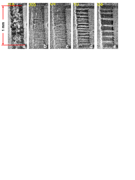
Figure 1: MO images taken at 2.5 K. Superconducting regions are black. ($H_{\parallel}$, $H_{\perp}$; in Oe): a, (0, 1); b, (60, 8); c, (100, 6); d, (110, 3); e, (115, 1.3).

The MO imaging was achieved using a set-up equipped with a 3D vector magnet Rinke2 . The sample was a 2.5 $\mu$m thick In film on a SiO₂ wafer. The film residual resistivity ratio was 540. The other film characteristics were the same as in Ref. VK, . Overall, the film is a Pippard superconductor ($\kappa\simeq 0.07$) in the pure limit. The sample length was 1 mm and the ratio width/thickness was 120, implying that for the perpendicular and parallel fields $\eta$ is $1$ and $0$, respectively. Images were taken simultaneously with measurements of the electrical resistance $R$ using a small low-frequency (11 Hz) AC current.

Typical images are presented in Fig. 1. The flux patterns are laminae independent of the history of the applied field. At $H_{\perp}\lesssim 1$ Oe fractionated laminae were seen in some runs. The laminae are planar and ordered at $H_{\parallel}\gtrsim 0.5H_{c}$. At smaller $H_{\parallel}$ ($=0.47H_{c}$ at 1.67 K) slight wave-like corrugations appear. In a perpendicular field the laminae are disordered (Fig. 1a). This suggests that the laminar structure is the ground state topology of the IS. The same conclusion was drawn by Faber Faber .

While $D_{n}$ ($D_{s}$) increases (decreases) and $R$ varies linearly with $H_{\perp}$, the period $D=D_{n}+D_{s}$, being dependent on $H_{\parallel}$, is constant for $0.3\lesssim H_{\perp}/H_{ic\perp}\lesssim 0.8$. Near $H_{\perp}=0$ and $H_{ci\perp}$ the number of laminae decreases. The IS-N transition for decreasing field is accompanied by deep supercooling of the N-state. This confirms the high purity of the sample and verifies that the IS-N transition is a first order phase transition Abrikosov .

Figure 2 presents the sample phase diagram $H_{c}(T)=H_{c\parallel}(T)$ measured with a DC magnetometer and used for in situ temperature determination. It is compared with data measured on other samples and the data from Ref. Finnemore, . The lower curve presents $H_{ci\perp}(T)$ at $H_{\parallel}=0$, determined from disappearance of the last S-lamina in the images and from $R(H_{\perp})$ measurements; the two perfectly coincide. As seen, $H_{ci\perp}(T)$ is less than half of $H_{c}(T)$. The stars represent $H_{ci\perp}$ calculated from Eq. (1) with $\xi_{0}$ = 380 nm and are clearly consistent with the experimental data. De Gennes’ formula yields $H_{ci\perp}$ considerably exceeding the experimental data. Hence we use Tinkham’s interpretation for the excess energy term.

The model. Since we adopt Tinkham’s approach and in agreement with the experimental images, the N- and S-domains are assumed to be rectangular parallelepipeds extending in the $H_{\parallel}$ direction. The contribution of the negative surface tension at the S/vacuum interface is neglected since the penetration depth is much less than the sample thickness. Magnetostriction effects are neglected as well. The out-of-plane and in-plane demagnetizing factors are $\eta_{\perp}=1$ and $\eta_{\parallel}=0$, respectively. The former means that $B_{\perp}\rho_{n}=H_{\perp}$ (conservation of the flux of the out-of-plane component of the magnetic field), whereas the latter means that $B_{\parallel}=H_{\parallel}$ and therefore the flux of $B_{\parallel}$ is not conserved. Hence, the appropriate thermodynamic potential is $\tilde{F}\equiv\tilde{f}V=F-V(B_{\parallel}H_{\parallel}/4\pi)=F-V_{n}(H_{\parallel}^{2}/4\pi)$, where $F$ is the free energy and the second term accounts for the work done by the generator to maintain $H_{\parallel}$ Landafshitz_II . This term is the key distinctive element of our model. We note that this term is neither small (it can exceed the condensation energy) nor trivial (its omission or incorrect form leads to violation of the limiting cases).

Summing the sample free energy at zero field $V[f_{n0}-H_{c}^{2}(1-\rho_{n})/8\pi)]$, the energy of the field $B$ in the sample $V\rho_{n}(B_{\perp}^{2}+B_{\parallel}^{2})/8\pi$, the energy of the S/N interfaces $V2\gamma/D$ and the excess energy of the field over the healing length $2VL_{h}(\rho_{n}B_{\perp}^{2}-H_{\perp}^{2})/8\pi d$, one obtains

$$\tilde{f}=f_{n0}-(1-\rho_{n})\frac{H_{c}^{2}}{8\pi}+\frac{H_{\perp}^{2}}{8\pi\rho_{n}}-\rho_{n}\frac{H_{\parallel}^{2}}{8\pi}+\\ 2\frac{H_{c}^{2}}{8\pi}\frac{\delta}{D}+2\frac{H_{\perp}^{2}}{8\pi}\frac{D}{d}(1-\rho_{n})^{2},$$ (3)

where $f_{n0}$ is the free energy density of the sample in the normal state at zero field.

Similar to the LLM, competition between the last two terms provides the equilibrium $D$:

$$D^{2}=\frac{d\delta}{\rho_{n}^{2}(1-\rho_{n})^{2}}\frac{H_{c}^{2}}{B_{\perp}^{2}}=\frac{d\delta}{(1-\rho_{n})^{2}}\frac{H_{c}^{2}}{H_{\perp}^{2}}.$$ (4)

Substituting (4) in (3) and then minimizing $\tilde{f}(\rho_{n})$ one obtains the equilibrium $\rho_{n}$:

$$\rho_{n}^{2}=h_{\perp}^{2}/(1-4h_{\perp}\sqrt{\delta/d}-h_{\parallel}^{2}).$$ (5)

where $h_{\perp}=H_{\perp}/H_{c}$ and $h_{\parallel}=H_{\parallel}/H_{c}$.

At the IS-N transition $\rho_{n}$=1, therefore

$$h_{ci\perp}=\sqrt{4(\delta/d)+1-h_{\parallel}^{2}}-2\sqrt{\delta/d}.$$ (6)

Finally, the reduced flux density $b=B/H_{c}$ is

$$b^{2}=b_{\perp}^{2}+b_{\parallel}^{2}=h_{\perp}^{2}/\rho_{n}^{2}+h_{\parallel}^{2}=1-4h_{\perp}\sqrt{\delta/d}.$$ (7)

The model satisfies the limiting cases, i.e., $\rho_{n}\rightarrow 0$ at $H_{\perp}\rightarrow 0$ and $H_{ci\perp}\rightarrow 0$ at $H_{\parallel}\rightarrow H_{c}$. In very thick samples ($\sqrt{\delta/d}\ll 1$) $B=H_{c}$ and Eq. (4) converts to Eq. (2) if $\rho_{n}^{2}(1-\rho_{n})^{2}$ is replaced by $f_{L}(\rho_{n})$; this explains the correctness of the temperature dependence $\delta(T)$ in Refs. Sharvin-Sn, ; Sharvin-In, .

For a perpendicular field ($H_{\parallel}=0$) we have that (a) according to Eq. (7) $B$ decreases with increasing $H$ from $H_{c}$ down to $H_{ci}$, in agreement with the $\mu$SR results Egorov ; and that (b) Eq. (6) reduces to Eq. (1), implying that the theoretical points in Fig. 2 are the same in our model. Hence, our model, developed for a regular laminar structure, can be used for irregular laminar patterns as well.

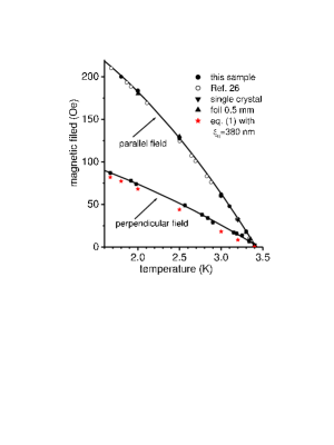
Figure 2: The phase diagram of our sample in parallel and perpendicular fields. The full curves are parabolic fits of the data obtained with our sample.

In Fig. 3 the data for $H_{ci\perp}$ at nonzero $H_{\parallel}$ are compared to the $H_{ci\perp}(H_{\parallel})$ dependence given by Eq. (6). We find that Eq. (6) correctly describes the experimental data.

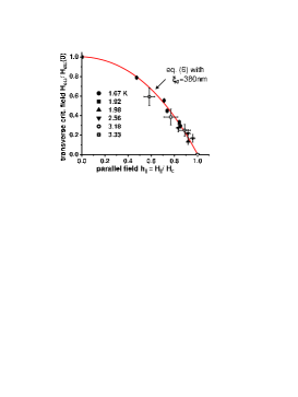
Figure 3: The perpendicular critical field $H_{ci\perp}/H_{ci\perp}(0)$ versus $h_{\parallel}=H_{\parallel}/H_{c}$. $H_{ci\perp}(0)$ is $H_{ci\perp}$ at $H_{\parallel}=0$.

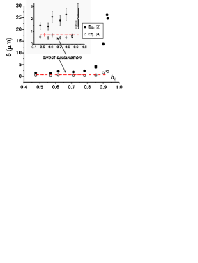
Figure 4: The domain-wall parameter $\delta$ inferred from MO images taken at $T$ = 1.7 K using Eq. (2) and Eq. (4) plotted on two scales. The dashed line represents the directly calculated $\delta=1.4\xi_{0}/(1-T/T_{c})^{0.5}$, $T_{c}=3.415$ K and $\xi_{0}=380$ nm.

Figure 4 presents the results for $\delta$ at $T$ = 1.7 K obtained in three ways. The circles represent $\delta$ calculated from Eq. (2) and Eq. (4) using our experimental data for the average $D$ and $H_{\perp}$ at $\rho_{n}=0.5$. The dashed line in Fig. 4 represents $\delta$ directly calculated using $\xi_{0}$ = 380 nm. We find that the results following from Eq. (4) agree with the directly calculated value of $\delta$. However this is not the case for $\delta$ obtained using Eq. (2).

Figure 5 presents data for the average $D$ obtained in two runs at $T=1.7\,K$ and $H_{\parallel}=0.85H_{c}$ and corresponding theoretical curves following from Eqs. (2) and (4). In Eq. (2) $D$ is controlled by $f_{L}$; in our model the spacing function is $f=(1-\rho_{n})^{2}h_{\perp}^{2}$ with $\rho_{n}$ and $h_{\perp}$ linked by Eq. (5). We find that both $f_{L}$ and $f$ qualitatively reproduce the experimental data. However $f_{L}$ “works” better at high values of $H_{\perp}/H_{ci\perp}$, whereas $f$ is better at small $H_{\perp}$. This indicates the importance of the rounded corners at high $H_{\perp}$, where inhomogeneity of $H_{\perp}$ is minimal.

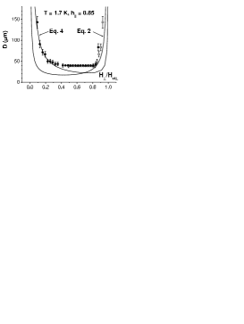
Figure 5: Experimental data (circles) and theoretical curves for the period of the laminar structure. Solid circles are the data obtained at increasing $H_{\perp}$ with the sample cooled at $H_{\perp}=0$. Open circles are the data taken after $H_{\perp}$ was reduced from above $H_{ci\perp}$ down to $0.5H_{ci\perp}$.

In summary, (i) we have performed a magneto-optical study of the IS in the high purity type-I superconductor resulting in a novel and comprehensive model of the IS for a slab in a tilted magnetic field, which includes the perpendicular field as the limiting case. The model is a good first order approximation of the IS in a slab as advanced by Landau many years ago. (ii) We have shown that a superconducting system in search for the lowest free energy may opt to keep $B$ in the bulk of N-domains considerably smaller than $H_{c}$. This alters the paradigm stating that this is impossible. In type-II superconductors the energy of the field $B$ in the vortex cores and the energy of the inhomogeneous field near the surface are composite parts of a sample free energy in the MS. Therefore variation of $B$ in the core and its dependents on the sample thickness can be expected in these materials as well. In particular, this can be a factor responsible for the observed dependence of the vortex core size on the applied field Sonier .

A weak point of our model is the oversimplified form of $L_{h}$ and neglect of the effect of the rounded corners. This is the main reason for the discrepancy between the experimental data and the theoretical curve in Fig. 5 and the deviation of $\rho_{n}(h_{\perp})$ in Eq. (6) from the linear dependence following from the linearity of $R(H_{\perp})$. To resolve this issue measurements of the magnetic field near the surface outside and inside the sample are required.

This work was supported by NSF (DMR 0904157) and by the Research Foundation – Flanders (FWO).

1. M. Seul and D. Andelman, Science 267, 476 (1995).
2. J. Ge, J. Gutierrez, B. Raes, J. Cuppens and V. V. Moshchalkov, New J. Phys. 15, 033013 (2013).
3. G. R. Berdiyorov, A. D. Hernández-Nieves, M. V. Milošević, F. M. Peeters, and D. Domínguez, Phys. Rev. B 85, 092502 (2012).
4. M. A. Engbarth, S. J. Bending, and M. V. Milošević, Phys. Rev. B 83, 224504 (2011).
5. G. R. Berdiyorov, A. D. Hernández, and F. M. Peeters, Phys. Rev. Lett. 103, 267002 (2009).
6. R. Prozorov, A. F. Fidler, J. R. Hobert, and P. C. Canfield, Nature Phys. 4, 327 (2008).
7. M. Tinkham, Introduction to Superconductivity (McGraw-Hill, 1996).
8. J. E. Sonier, W. Huang, C.V. Kaiser, C. Cochrane, V. Pacradouni, S. A. Sabok-Sayr, M. D. Lumsden, B. C. Sales, M. A. McGuire, A. S. Sefat, and D. Mandrus, Phys. Rev. Lett. 106, 127002 (2011).
9. A. A. Abrikosov, Fundamentals of the Theory of Metals (Elsevier Science Pub. Co., 1988).
10. J. Pearl, Appl. Phys. Lett. 5, 65 (1964).
11. R. E. Goldstein, D. P. Jackson, A. T. Dorsey, Phys. Rev. Lett. 76, 3818 (1996).
12. L. D. Landau, Zh.E.T.F. 7, 371 (1937).
13. R. Prozorov, Phys. Rev. Lett. 98, 257001 (2007).
14. C. J. Gorter and H. Casimir, Physica 1, 306 (1934).
15. L. D. Landau, E.M. Lifshitz and L. P. Pitaevskii, Electrodynamics of Continuous Media, 2nd ed. (Elsevier, 1984).
16. P. G. De Gennes, Superconductivity of Metals and Alloys (Perseus Book Publishing, L.L.C., 1966).
17. R. P. Huebener Magnetic Flux Structures in Superconductors, 2nd ed. (Springer-Verlag, 2001).
18. I. T. Faber, Proc. Roy. Soc. A 248, 460 (1958).
19. V. Kozhevnikov, A. Suter, H. Fritzsche, V. Gladilin, A. Volodin, T. Moorkens, M. Trekels, J. Cuppens, B. M. Wojek, T. Prokscha, E. Morenzoni, G. J. Nieuwenhuys, M. J. Van Bael, K. Temst, C. Van Haesendonck, J. O. Indekeu, Phys. Rev. B87, 104508 (2013).
20. Yu. V. Sharvin, Zh.E.T.F. 33, 1341 (1957) [Sov. Phys. JETP 33, 1031 (1958)].
21. Yu. V. Sharvin, Zh.E.T.F. 38, 298 (1960) [Sov. Phys. Jetp 11, 316 (1960)].
22. L. D. Landau, Nature 147, 688 (1938); Zh.E.T.F. 13, 377 (1943).
23. A. Fortini and E. Paumier, Phys. Rev. B 5, 1850 (1972).
24. V. S. Egorov, G. Solt, C. Baines, D. Herlach, and U. Zimmermann, Phis. Rev. B 64, 024524 (2001).
25. R. Wijngaarden, C. Aegerter, M. Welling, K. Heeck, in Magneto-Optical Imaging, T. H. Johansen, D. V. Shantsev (eds.), (Kluwer Academic, 2003).
26. D. K. Finnemore, and D. E. Mapother, Phys. Rev. 140, A507 (1965).
27. J. E. Sonier, Rep. Prog. Phys. 70, 1717 (2007).