Asymptotic and measured large frequency separations

Abstract

Context. With the space-borne missions CoRoT and Kepler, a large amount of asteroseismic data is now available and has led to a variety of work. So-called global oscillation parameters are inferred to characterize the large sets of stars, perform ensemble asteroseismology, and derive scaling relations. The mean large separation is such a key parameter, easily deduced from the radial-frequency differences in the observed oscillation spectrum and closely related to the mean stellar density. It is therefore crucial to measure it with the highest accuracy in order to obtain the most precise asteroseismic indices.

Aims. As the conditions of measurement of the large separation do not coincide with its theoretical definition, we revisit the asymptotic expressions used for analyzing the observed oscillation spectra. Then, we examine the consequence of the difference between the observed and asymptotic values of the mean large separation.

Methods. The analysis is focused on radial modes. We use series of radial-mode frequencies in published analyses of stars with solar-like oscillations to compare the asymptotic and observational values of the large separation. This comparison relies on the proper use of the second-order asymptotic expansion.

Results. We propose a simple formulation to correct the observed value of the large separation and then derive its asymptotic counterpart. The measurement of the curvature of the radial ridges in the échelle diagram provides the correcting factor. We prove that, apart from glitches due to stellar structure discontinuities, the asymptotic expansion is valid from main-sequence stars to red giants. Our model shows that the asymptotic offset is close to 1/4, as in the theoretical development, for low-mass, main-sequence stars, subgiants and red giants.

Conclusions. High-quality solar-like oscillation spectra derived from precise photometric measurements are definitely better described with the second-order asymptotic expansion. The second-order term is responsible for the curvature observed in the échelle diagrams used for analyzing the oscillation spectra, and this curvature is responsible for the difference between the observed and asymptotic values of the large separation. Taking it into account yields a revision of the scaling relations, which provides more accurate asteroseismic estimates of the stellar mass and radius. After correction of the bias (6 % for the stellar radius and 3 % for the mass), the performance of the calibrated relation is about 4 % and 8 % for estimating, respectively, the stellar radius and the stellar mass for masses less than $1.3\,M_{\odot}$; the accuracy is twice as bad for higher mass stars and red giants.

1 Introduction

The amount of asteroseismic data provided by the space-borne missions CoRoT and Kepler has given rise to ensemble asteroseismology. With hundreds of stars observed from the main sequence to the red giant branch, it is possible to study evolutionary sequences and to derive seismic indices from global seismic observational parameters. These global parameters can be measured prior to any complete determination of the individual mode frequencies and are able to provide global information on the oscillation spectra (e.g., Michel et al. 2008). For instance, the mean large separation $\Delta\nu$ between consecutive radial-mode frequencies and the frequency $\nu_{\mathrm{max}}$ of maximum oscillating signal are widely used to provide estimates of the stellar mass and radius (e.g., Kallinger et al. 2010; Mosser et al. 2010). Almost all other scaling relations make use of $\Delta\nu$, as, for instance, the scaling reations governing the amplitude of the oscillation signal (e.g., Stello et al. 2011; Mosser et al. 2012a). In case an oscillation spectrum is determined with a low signal-to-noise ratio, the mean large separation is the single parameter that can be precisely measured (e.g., Bedding et al. 2001; Mosser et al. 2009; Gaulme et al. 2010).

The definition of the large separation relies on the asymptotic theory, valid for large values of the eigenfrequencies, corresponding to large values of the radial order. However, its measurement is derived from the largest peaks seen in the oscillation spectrum in the frequency range surrounding $\nu_{\mathrm{max}}$, thus in conditions that do not directly correspond to the asymptotic relation. This difference can be taken into account in comparisons with models for a specific star, but not in the consideration of large sets of stars for statistical studies.

In asteroseismology, ground-based observations with a limited frequency resolution have led to the use of simplified and incomplete forms of the asymptotic expansion. With CoRoT and Kepler data, these simplified forms are still in use, but observed uncertainties on frequencies are much reduced. As for the Sun, one may question using the asymptotic expansion, since the quality of the data usually allows one to go beyond this approximate relation. Moreover, modeling has shown that acoustic glitches due to discontinuities or important gradients in the stellar structure may hamper the use of the asymptotic expansion (e.g., Audard & Provost 1994).

In this work, we aim to use the asymptotic relation in a proper way to derive the generic properties of a solar-like oscillation spectrum. It seems therefore necessary to revisit the different forms of asymptotic expansion since $\Delta\nu$ is introduced by the asymptotic relation. We first show that it is necessary to use the asymptotic expansion including its second-order term, without simplification compared to the theoretical expansion. Then, we investigate the consequence of measuring the large separation at $\nu_{\mathrm{max}}$ and not in asymptotic conditions. The relation between the two values, $\Delta\nu_{\mathrm{as}}$ for the asymptotic value and $\Delta\nu_{\mathrm{obs}}$ for the observed one, is developed in Section 2. The analysis based on radial-mode frequencies found in the literature is carried out in Section 3 to quantify the relation between the observed and asymptotic parameters, under the assumption that the second-order asymptotic expansion is valid for describing the radial oscillation spectra. We verify that this hypothesis is valid when we consider two regimes, depending on the stellar evolutionary status. We discuss in Section 4 the consequences of the relation between the observed and asymptotic parameters. We also use the comparison of the seismic and modeled values of the stellar mass and radius to revise the scaling relations providing $M$ and $R$ estimates.

Figure 1: Échelle diagram of the radial modes of the star KIC 9139163 (from Appourchaux et al. 2012). The red dashed line indicates the quadratic fit that mimics the curvature.

Figure 2: Variation of the large separations $\nu_{n+1,0}-\nu_{n,0}$ as a function of $\nu_{n,0}$ for the star HD 49933 (from Benomar et al. 2009). The red dashed line indicates a linear fit.

2 Asymptotic relation versus observed parameters

2.1 The original asymptotic expression

The oscillation pattern of low-degree oscillation pressure modes can be described by a second-order relation (Eqs. 65-74 of Tassoul 1980). This approximate relation is called asymptotic, since its derivation is strictly valid only for large radial orders. The development of the eigenfrequency $\nu_{n,\ell}$ proposed by Tassoul includes a second-order term, namely, a contribution in $1/\nu_{n,\ell}$:

$$\nu_{n,\ell}=\left(n+{\ell\over 2}+\varepsilon\right)\;\Delta\nu-\left[\ell(\ell+1)\;d_{0}+d_{1}\right]{\Delta\nu^{2}\over\nu_{n,\ell}}$$ (1)

where $n$ is the p-mode radial order, $\ell$ is the angular degree, $\Delta\nu$ is the large separation, and $\varepsilon$ is a constant term. The terms $\Delta\nu$ and $\varepsilon$ are discussed later; the dimensionless term $d_{0}$ is related to the gradient of sound speed integrated over the stellar interior; $d_{1}$ has a complex form.

2.2 The asymptotic expansion used in practice

When reading the abundant literature on asteroseismic observations, the most common forms of the asymptotic expansion used for interpreting observed low-degree oscillation spectra (e.g., Mosser et al. 1991; Bedding et al. 2001; Bouchy et al. 2005, for ground-based observations) are similar to the approximate form

$$\nu_{n,\ell}\simeq\left(n+{\ell\over 2}+\varepsilon_{0}\right)\;\Delta\nu_{0}-\ell(\ell+1)\;D_{0}.$$ (2)

Compared to Eq. (1), the contribution of $d_{1}$ and the variation of the denominator varying as $\nu_{n,\ell}$ are both omitted. This omission derives from the fact that ground-based observations have a too coarse frequency resolution. Equation (2) is still in use for space-borne observations that provide a much better frequency resolution (e.g., Campante et al. 2011; White et al. 2012; Corsaro et al. 2012). The large separation $\Delta\nu_{0}$ and the offset $\varepsilon_{0}$ are supposed to play the roles of $\Delta\nu$ and $\varepsilon$ in Eq. (1): this is not strictly exact, as shown later.

Observationally, the terms $\Delta\nu_{0}$ and $D_{0}$ can be derived from the mean frequency differences

$$\Delta\nu_{0} = \langle\nu_{n+1,\ell}-\nu_{n,\ell}\rangle,$$ (3)

$$D_{0} = \langle{1\over 4\ell+6}\,(\nu_{n,\ell}-\nu_{n-1,\ell+2})\rangle,$$ (4)

where the square brackets represent the mean values in the observed frequency range. For radial modes, the asymptotic expansion reduces to

$$\nu_{n,0}=\left(n+\varepsilon_{0}\right)\;\Delta\nu_{0}.$$ (5)

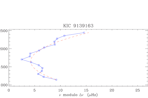
Clearly, this form cannot account for an accurate description of the radial-mode pattern, since the échelle diagram representation shows an noticeable curvature for most stars with solar-like oscillations at all evolutionary stages. This curvature, always with the same concavity sign, is particularly visible in red giant oscillations (e.g., Mosser et al. 2011; Kallinger et al. 2012), which show solar-like oscillations at low radial order (e.g., De Ridder et al. 2009; Bedding et al. 2010a). Figure 1 shows a typical example of the non-negligible curvature in the échelle diagram of a main-sequence star with many radial orders. The concavity corresponds equivalently to a positive gradient of the large separation (Fig. 2). This gradient is not reproduced by Eq. (5), stressing that this form of the asymptotic expansion is not adequate for reporting the global properties of the radial modes observed with enough precision. Hence, it is necessary to revisit the use of the asymptotic expression for interpreting observations and to better account for the second-order term.

2.3 Radial modes depicted by second-order asymptotic expansion

We have chosen to restrict the analysis to radial modes. We express the second-order term varying in $\nu^{-1}$ of Eq. (1) with a contribution in $n^{-1}$:

$$\nu_{n,0}=\left(n+\varepsilon_{\mathrm{as}}+{A_{\mathrm{as}}\over n}\right)\;\Delta\nu_{\mathrm{as}}.$$ (6)

Compared to Eq. (1), we added the subscript $as$ to the different terms in order to make clear that, contrary to Eq. (2), we respect the asymptotic condition. We replaced the second-order term in $1/\nu$ by a term in $1/n$ instead of $1/(n+\varepsilon_{\mathrm{as}})$, since the contribution of $\varepsilon_{\mathrm{as}}$ in the denominator can be considered as a third-order term in $n$.

The large separation $\Delta\nu_{\mathrm{as}}$ is related to the stellar acoustic diameter by

$$\Delta\nu_{\mathrm{as}}=\left(2\int_{0}^{R}{\mathrm{d}r\over c}\right)^{-1},$$ (7)

where $c$ is the sound speed. We note that $\Delta\nu_{0}$, different from the asymptotic value $\Delta\nu_{\mathrm{as}}$, cannot directly provide the integral value of $1/c$. We also note that the offset $\varepsilon_{\mathrm{as}}$ has a fixed value in the original work of Tassoul:

$$\varepsilon_{\mathrm{as}}{}_{\mathrm{,Tassoul}}={1\over 4}.$$ (8)

In the literature, one also finds that $\varepsilon_{\mathrm{as}}=1/4+a(\nu)$, where $a(\nu)$ is determined by the properties of the near-surface region (Christensen-Dalsgaard & Perez Hernandez 1992).

The second-order expansion is valid for large radial orders only, when the second-order term $A_{\mathrm{as}}/n$ is small. This means that the large separation $\Delta\nu_{\mathrm{as}}$ corresponds to the frequency difference between radial modes at high frequency only, but not at $\nu_{\mathrm{max}}$. We note that the second-order term can account for the curvature of the radial ridge in the échelle diagram, with a positive value of $A_{\mathrm{as}}$ for reproducing the sign of the observed concavity.

Figure 3: Échelle diagrams of the radial modes of a typical red-clump giant, comparing the asymptotic expansion (Eq. (6), blue triangles) and the development describing the curvature (Eq. 9, red diamonds). Top: diagram based on $\Delta\nu_{\mathrm{obs}}$ observed at $\nu_{\mathrm{max}}$; the dashed line indicates the vertical asymptotic line at $\nu_{\mathrm{max}}$; the dot-dashed line indicates the asymptotic line at high frequency. For clarity, the ridge has been duplicated modulo $\Delta\nu_{\mathrm{obs}}$. Bottom: diagram based on $\Delta\nu_{\mathrm{as}}$; the dot-dashed line indicates the vertical asymptotic line at high frequency.

2.4 Taking into account the curvature

In practice, the large separation is necessarily obtained from the radial modes with the largest amplitudes observed in the oscillation pattern around $\nu_{\mathrm{max}}$ (e.g., Mosser & Appourchaux 2009). In order to reconcile observations at $\nu_{\mathrm{max}}$ and asymptotic expansion at large frequency, we must first consider the curvature of the ridge. To enhance the quality of the fit of radial modes in red giants, Mosser et al. (2011) have proposed including the curvature of the radial ridge with the expression

$$\nu_{n,0}=\left(n+\varepsilon_{\mathrm{obs}}+{\alpha_{\mathrm{obs}}\over 2}\;[n-n_{\mathrm{max}}]^{2}\right)\Delta\nu_{\mathrm{obs}},$$ (9)

where $\Delta\nu_{\mathrm{obs}}$ is the observed large separation, measured in a wide frequency range around the frequency $\nu_{\mathrm{max}}$ of maximum oscillation amplitude, $\alpha_{\mathrm{obs}}$ is the curvature term, and $\varepsilon_{\mathrm{obs}}$ is the offset. We have also introduced the dimensionless value of $\nu_{\mathrm{max}}$, defined by $n_{\mathrm{max}}=\nu_{\mathrm{max}}/\Delta\nu_{\mathrm{obs}}$. Similar fits have already been proposed for the oscillation spectra of the Sun (Christensen-Dalsgaard & Frandsen 1983; Grec et al. 1983; Scherrer et al. 1983), of $\alpha$ Cen A (Bedding et al. 2004), $\alpha$ Cen B (Kjeldsen et al. 2005), HD 203608 (Mosser et al. 2008b), Procyon (Mosser et al. 2008a), and HD 46375 (Gaulme et al. 2010). In fact, such a fit mimics a second-order term and provides a linear gradient in large separation:

$${\nu_{n+1,0}-\nu_{n-1,0}\over 2}=\left(1+\alpha_{\mathrm{obs}}\left[n-n_{\mathrm{max}}\right]\right)\Delta\nu_{\mathrm{obs}}.$$ (10)

The introduction of the curvature may be considered as an empirical form of the asymptotic relation. It reproduces the second-order term of the asymptotic expansion, which has been neglected in Eq. (2), with an unequivocal correspondence. It relies on a global description of the oscillation spectrum, which considers that the mean values of the seismic parameters are determined in a large frequency range around $\nu_{\mathrm{max}}$ (Mosser & Appourchaux 2009). Such a description has shown interesting properties when compared to a local one that provides the large separation from a limited frequency range only around $\nu_{\mathrm{max}}$ (Verner et al. 2011; Hekker et al. 2012).

It is straightforward to make the link between both asymptotic and observed descriptions of the radial oscillation pattern with a second-order development in $(n-n_{\mathrm{max}})/n_{\mathrm{max}}$ of the asymptotic expression. From the identification of the different orders in Eqs. (6) and (9) (constant, varying in $n$ and in $n^{2}$), we then get

$$\Delta\nu_{\mathrm{as}} = \Delta\nu_{\mathrm{obs}}\ \left({1+{n_{\mathrm{max}}\alpha_{\mathrm{obs}}\over 2}}\right),$$ (11)

$$A_{\mathrm{as}} = {\alpha_{\mathrm{obs}}\over 2}{n_{\mathrm{max}}^{3}\over 1+n_{\mathrm{max}}\displaystyle{\alpha_{\mathrm{obs}}\over 2}},$$ (12)

$$\varepsilon_{\mathrm{as}} = {\varepsilon_{\mathrm{obs}}-n_{\mathrm{max}}^{2}\alpha_{\mathrm{obs}}\over 1+n_{\mathrm{max}}\displaystyle{\alpha_{\mathrm{obs}}\over 2}}.$$ (13)

When considering that the ridge curvature is small enough $(n_{\mathrm{max}}\alpha_{\mathrm{obs}}/2\ll 1)$, $A_{\mathrm{as}}$ and $\varepsilon_{\mathrm{as}}$ become

$$A_{\mathrm{as}} \simeq {\alpha_{\mathrm{obs}}\over 2}\ n_{\mathrm{max}}^{3},$$ (14)

$$\varepsilon_{\mathrm{as}} \simeq \varepsilon_{\mathrm{obs}}\left({1-{n_{\mathrm{max}}\alpha_{\mathrm{obs}}\over 2}}\right)-n_{\mathrm{max}}^{2}\alpha_{\mathrm{obs}}.$$ (15)

These developments provide a reasonable agreement with the previous exact correspondence between the asymptotic and observed forms.

The difference between the observed and asymptotic values of $\varepsilon$ includes a systematic offset in addition to the rescaling term $\left({1-{n_{\mathrm{max}}\alpha_{\mathrm{obs}}/2}}\right)$. This comes from the fact that the measurement of $\varepsilon_{\mathrm{obs}}$ significantly depends on the measurement of $\Delta\nu_{\mathrm{obs}}$: a relative change $\eta$ in the measurement of the large separation translates into an absolute change of the order of $-n_{\mathrm{max}}\eta$. This indicates that the measurement of $\varepsilon_{\mathrm{obs}}$ is difficult since it includes large uncertainties related to all effects that affect the measurement of the large separation, such as structure discontinuities or significant gradients of composition (Miglio et al. 2010; Mazumdar et al. 2012).

2.5 Échelle diagrams

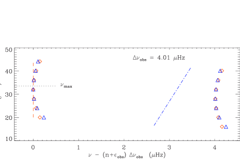
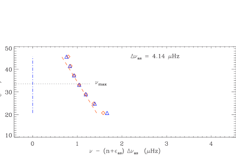
The échelle diagrams in Fig. 3 compare the radial oscillation patterns folded with $\Delta\nu_{\mathrm{obs}}$ or $\Delta\nu_{\mathrm{as}}$. In practice, the folding is naturally based on the observations of quasi-vertical ridges and provides $\Delta\nu_{\mathrm{obs}}$ observed at $\nu_{\mathrm{max}}$ (Fig. 3 top). A folding based on $\Delta\nu_{\mathrm{as}}$ would not show any vertical ridge in the observed domain (Fig. 3 bottom). In Fig. 3 we have also compared the asymptotic spectrum based on the parameters $\Delta\nu_{\mathrm{as}}$, $A_{\mathrm{as}}$, and $\varepsilon_{\mathrm{as}}$ to the observed spectrum, obeying Eq. (9). Perfect agreement is naturally met for $\nu\simeq\nu_{\mathrm{max}}$. Differences vary as $\alpha_{\mathrm{obs}}(n-n_{\mathrm{max}})^{3}$. They remain limited to a small fraction of the large separation, even for the orders far from $n_{\mathrm{max}}$, so that the agreement of the simplified expression is satisfactory in the frequency range where modes have appreciable amplitudes. Comparison of the échelle diagrams illustrates that the observable $\Delta\nu_{\mathrm{obs}}$ significantly differs from the physically-grounded asymptotic value $\Delta\nu_{\mathrm{as}}$.

3 Data and analysis

3.1 Observations: main-sequence stars and subgiants

Published data allowed us to construct a table of observed values of $\alpha_{\mathrm{obs}}$ and $\varepsilon_{\mathrm{obs}}$ as a function of the observed large separation $\Delta\nu_{\mathrm{obs}}$ (Table LABEL:valeurs, with 94 stars). We considered observations of subgiants and main-sequence stars observed by CoRoT or by Kepler. We also made use of ground-based observations and solar data. All references are given in the caption of Table LABEL:valeurs.

We have considered the radial eigenfrequencies, calculated local large spacings $\nu_{n+1,0}-\nu_{n,0}$, and derived $\Delta\nu_{\mathrm{obs}}$ and $\alpha_{\mathrm{obs}}$ from a linear fit corresponding to the linear gradient given by Eq. (10). The term $\varepsilon_{\mathrm{obs}}$ is then derived from Eq. (9). With the help of Eqs. (11), (12) and (13), we analyzed the differences between the observables $\Delta\nu_{\mathrm{obs}}$, $\varepsilon_{\mathrm{obs}}$, $\alpha_{\mathrm{obs}}$ and their asymptotic counterparts $\Delta\nu_{\mathrm{as}}$, $\varepsilon_{\mathrm{as}}$, and $A_{\mathrm{as}}$. We have chosen to express the variation with the parameter $n_{\mathrm{max}}$, rather than $\Delta\nu_{\mathrm{obs}}$ or $\nu_{\mathrm{max}}$. Subgiants have typically $n_{\mathrm{max}}\geq 15$, and main-sequence stars $n_{\mathrm{max}}\geq 18$.

3.2 Observations: red giants

We also considered observations of stars on the red giant branch that have been modelled. They were analyzed exactly as the less-evolved stars. However, this limited set of stars cannot represent the diversity of the thousands of red giants already analyzed in both the CoRoT and Kepler fields (e.g., Hekker et al. 2009; Bedding et al. 2010a; Mosser et al. 2010; Stello et al. 2010). We note, for instance, that their masses are higher than the mean value of the largest sets. Furthermore, because the number of excited radial modes is much more limited than for main-sequence stars (Mosser et al. 2010), the observed seismic parameters suffer from a large spread. Therefore, we also made use of the mean relation found for the curvature of the red giant radial oscillation pattern (Mosser et al. 2012b)

$${\alpha_{\mathrm{obs}}}{}_{\mathrm{,RG}}=0.015\ \Delta\nu_{\mathrm{obs}}^{-0.32}.$$ (16)

This relation, when expressed as a function of $n_{\mathrm{max}}$ and taking into account the scaling relation $\Delta\nu\propto\nu_{\mathrm{max}}^{0.75}$ (e.g., Hekker et al. 2011), gives ${\alpha_{\mathrm{obs}}}{}_{\mathrm{,RG}}=0.09\ n_{\mathrm{max}}^{-0.96}$. The exponent of this scaling relation is close to $-1$, so that for the following study we simply consider the fit

$${\alpha_{\mathrm{obs}}}{}_{\mathrm{,RG}}=2\,a{}_{\mathrm{RG}}\,n_{\mathrm{max}}^{-1},$$ (17)

with $a{}_{\mathrm{RG}}=0.038\pm 0.002$. Red giants have typically $n_{\mathrm{max}}\leq 15$.

Figure 4: Curvature $10^{3}\ \alpha_{\mathrm{obs}}$ as a function of $n_{\mathrm{max}}=\nu_{\mathrm{max}}/\Delta\nu$. The thick line corresponds to the fit in $n_{\mathrm{max}}^{-1}$ established for red giants, and the dotted line to its extrapolation towards larger $n_{\mathrm{max}}$. The dashed line provides an acceptable fit in $n_{\mathrm{max}}^{-2}$ valid for main-sequence stars. Error bars indicate the typical 1-$\sigma$ uncertainties in three different domains. The color code of the symbols provides an estimate of the stellar mass; the colors of the lines correspond to the different regimes.

Figure 5: Same as Fig. 4, for the second-order asymptotic term $A_{\mathrm{as}}$ as a function of $n_{\mathrm{max}}$. The fits of $A_{\mathrm{as}}$ in the different regimes are derived from the fits of $\alpha_{\mathrm{obs}}$ in Fig. 4 and the relation provided by Eq. (12).

Figure 6: Same as Fig. 4, for the relative difference of the large separations, equivalent to $n_{\mathrm{max}}\alpha_{\mathrm{obs}}/2$, as a function of $n_{\mathrm{max}}$.

3.3 Second-order term $A_{\mathrm{as}}$ and curvature $\alpha_{\mathrm{obs}}$

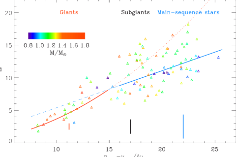
We first examined the curvature $\alpha_{\mathrm{obs}}$ as a function of $n_{\mathrm{max}}$ (Fig. 4), since this term governs the relation between the asymptotic and observed values of the large separation (Eq. (11)). A large spread is observed because of the acoustic glitches caused by structure discontinuities (e.g., Miglio et al. 2010). Typical uncertainties of $\alpha_{\mathrm{obs}}$ are about 20 %. We are interested in the mean variation of the observed and asymptotic parameters, so that the glitches are first neglected and later considered in Section 4.1. The large spread of the data implies that, as is well known, the asymptotic expansion cannot precisely relate all of the features of a solar-like oscillation spectrum. However, this spread does not invalidate the analysis of the mean evolution of the observed and asymptotic parameters with frequency.

The fit of $\alpha_{\mathrm{obs}}$ derived from red giants, valid when $n_{\mathrm{max}}$ is in the range [7, 15], does not hold for less-evolved stars with larger $n_{\mathrm{max}}$ (Fig. 4). It could reproduce part of the observed curvature of subgiants but yields too large values in the main-sequence domain. In order to fit main-sequence stars and subgiants, it seems necessary to modify the exponent of the relation $\alpha_{\mathrm{obs}}(n_{\mathrm{max}})$. When restricted to main-sequence stars, the fit of $\alpha_{\mathrm{obs}}(n_{\mathrm{max}})$ provides an exponent of about $-2\pm 0.3$. We thus chose to fix the exponent to the integer value $-2$:

$${\alpha_{\mathrm{obs}}}{}_{\mathrm{,MS}}=2\,a{}_{\mathrm{MS}}\,n_{\mathrm{max}}^{-2},$$ (18)

with $a{}_{\mathrm{MS}}=0.57\pm 0.02$. Having a different fit compared to the red giant case (Eq. (16)) is justified in Section 3.5: even if a global fit in $n_{\mathrm{max}}^{-1.5}$ should reconcile the two regimes, we keep the two regimes since we also have to consider the fits of the other asymptotic parameters, especially $\varepsilon_{\mathrm{obs}}$. We also note a gradient in mass: low-mass stars have systematically lower $\alpha_{\mathrm{obs}}$ than high-mass stars. Masses were derived from the seismic estimates when modeled masses are not available (Table LABEL:valeurs). At this stage, it is however impossible to take this mass dependence into consideration.

As a consequence of Eq. (14), we find that the second-order asymptotic term $A_{\mathrm{as}}$ scales as $n_{\mathrm{max}}^{2}$ for red giants and as $n_{\mathrm{max}}$ for less-evolved stars (Fig. 5). We note, again, a large spread of the values, which is related to the acoustic glitches.

3.4 Large separations $\Delta\nu_{\mathrm{as}}$ and $\Delta\nu_{\mathrm{obs}}$

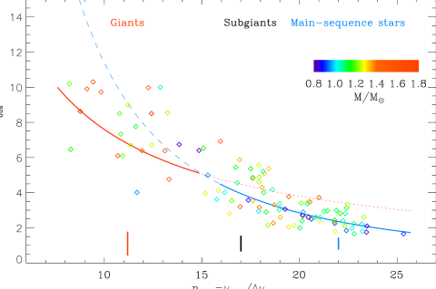
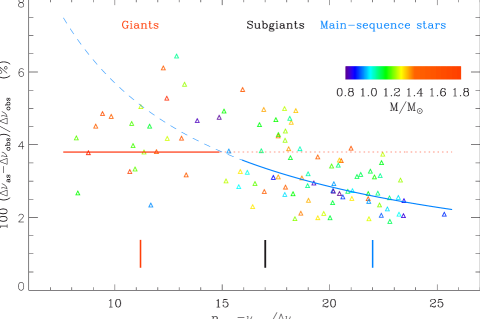
The asymptotic and observed values of the large separations of the set of stars are clearly distinct (Fig. 6). According to Eq. (11), the correction from $\Delta\nu_{\mathrm{obs}}$ to $\Delta\nu_{\mathrm{as}}$ has the same relative uncertainty as $\alpha_{\mathrm{obs}}$. The relative difference between $\Delta\nu_{\mathrm{as}}$ and $\Delta\nu_{\mathrm{obs}}$ increases when $n_{\mathrm{max}}$ decreases and reaches a constant maximum value of about 4 % in the red giant regime, in agreement with Eq. (17). Their difference is reduced at high frequency for subgiants and main-sequence stars, as in the solar case, where high radial orders are observed, but still of the order to 2 %. This relative difference, even if small, depends on the frequency. This can be represented, for the different regimes, by the fit

$$\Delta\nu_{\mathrm{as}}=\left(1+\zeta\right)\ \Delta\nu_{\mathrm{obs}},$$ (19)

with

$$\zeta = \displaystyle{0.57\over n_{\mathrm{max}}}\qquad\hbox{(main-sequence regime: }n_{\mathrm{max}}\geq 15),$$ (20)

$$\zeta = 0.038\qquad\ \ \hbox{(red giant regime: }n_{\mathrm{max}}\leq 15).$$ (21)

The consequence of these relations is examined in Section 4.2. As for the curvature, the justification of the two different regimes is based on the analysis of the offset $\varepsilon_{\mathrm{obs}}$.

Figure 7: Same as Fig. 4, for the observed (diamonds) and asymptotic (triangles) offsets. Both parameters are fitted, with dotted lines in the red giant regime and dashed lines in the main-sequence regime; thicker lines indicate the domain of validity of the fits. The triple-dot-dashed line represents the Tassoul value $\varepsilon_{\mathrm{as}}=1/4$, and the dot-dashed line is the model of $\varepsilon_{\mathrm{obs}}$ (varying with $\log\Delta\nu_{\mathrm{obs}}$ in the red giant regime, and constant for less-evolved stars).

Figure 8: Same as Fig. 7, with a color code depending on the effective temperature.

3.5 Observed and asymptotic offsets

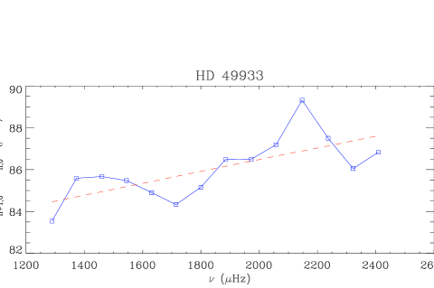
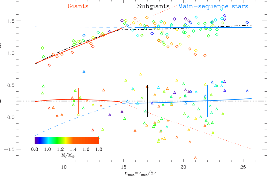
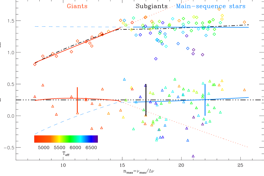
The offsets $\varepsilon_{\mathrm{obs}}$ and $\varepsilon_{\mathrm{as}}$ are plotted in Fig. 7. The fit of $\varepsilon_{\mathrm{obs}}$, initially given by Mosser et al. (2011) for red giants and updated by Corsaro et al. (2012), is prolonged to main-sequence stars with a nearly constant fit at $\varepsilon_{\mathrm{obs}}{}_{\mathrm{,MS}}\simeq 1.4$. We based this fit on low-mass G stars in order to avoid the more complex spectra of F stars that can be affected by the HD 49933 misidentification syndrome (Appourchaux et al. 2008; Benomar et al. 2009). The spread of $\varepsilon_{\mathrm{as}}$ is large since the propagation of the uncertainties from $\alpha_{\mathrm{obs}}$ to $\varepsilon_{\mathrm{as}}$ yields a large uncertainty: $\delta\varepsilon_{\mathrm{as}}\simeq 2\delta\alpha_{\mathrm{obs}}/\alpha_{\mathrm{obs}}\simeq 0.4$.

We note in particular that the two different regimes seen for $\alpha_{\mathrm{obs}}$ correspond to the different variations of $\varepsilon_{\mathrm{obs}}$ with stellar evolution. The comparison between $\varepsilon_{\mathrm{as}}$ and $\varepsilon_{\mathrm{obs}}$ allows us to derive significant features. The regime where $\varepsilon_{\mathrm{obs}}$ does not change with $\Delta\nu_{\mathrm{obs}}$ coincides with the regime where the curvature evolves with $n_{\mathrm{max}}^{-2}$. The correction provided by Eq. (13) then mainly corresponds to the constant term $2\,a{}_{\mathrm{MS}}$. As a consequence, for low-mass main-sequence and subgiant stars the asymptotic value is very close to 1/4 (Eq. (8), as found by Tassoul 1980). In the red-giant regime, the curvature varying as $n_{\mathrm{max}}^{-1}$ provides a variable correction, so that $\varepsilon_{\mathrm{as}}$ is close to 1/4 also even if $\varepsilon_{\mathrm{obs}}$ varies with $\Delta\nu_{\mathrm{obs}}$.

3.6 Mass dependence

For low-mass stars, the fact that we find a mean value $\langle\varepsilon_{\mathrm{as}}\rangle$ of about 1/4 suggests that the asymptotic expansion is valid for describing solar-like oscillation spectra in a coherent way. This validity is also confirmed for red giants. For those stars, we may assume that $\varepsilon_{\mathrm{as}}\equiv 1/4$. Having the observed value $\varepsilon_{\mathrm{obs}}$ much larger than $\varepsilon_{\mathrm{as}}$ can be seen as an artefact of the curvature $\alpha_{\mathrm{obs}}$ introduced by the use of $\Delta\nu_{\mathrm{obs}}$:

$$\varepsilon_{\mathrm{obs}}\simeq{1\over 4}\left(1+n_{\mathrm{max}}\displaystyle{\alpha_{\mathrm{obs}}\over 2}\right)+n_{\mathrm{max}}^{2}\alpha_{\mathrm{obs}}.$$ (22)

However, we note in Fig. 7 a clear gradient of $\varepsilon_{\mathrm{as}}$ with the stellar mass: high-mass stars have in general lower $\varepsilon_{\mathrm{as}}$ than low-mass stars, similar to what is observed for $\varepsilon_{\mathrm{obs}}$. In massive stars, the curvature is more pronounced; $\varepsilon_{\mathrm{obs}}$ and $\varepsilon_{\mathrm{as}}$ are lower than in low-mass stars. As a consequence, the asymptotic value $\varepsilon_{\mathrm{as}}$ cannot coincide with 1/4, as is approximately the case for low-mass stars. We tried to reconcile this different behavior by taking into account a mass dependence in the fit of the curvature. In fact, fitting the higher curvature of high-mass stars would translate into a larger correction, in absolute value, from $\varepsilon_{\mathrm{obs}}$ to $\varepsilon_{\mathrm{as}}$, so that it cannot account for the difference.

We are therefore left with the conclusion that, contrary to low-mass stars, the asymptotic expansion is less satisfactory for describing the radial-mode oscillation spectra of high-mass stars. At this stage, we may imagine that in fact some features are superimposed on the asymptotic spectrum, such as signatures of glitches with longer period than the radial-order range where the radial modes are observed. Such long-period glitches can be due to the convective core in main-sequence stars with a mass larger than 1.2 $M_{\odot}$; they are discussed in Section 4.1.

4 Discussion

We explore here some consequences of fitting the observed oscillation spectra with the exact asymptotic relation. First, we examine the possible limitations of this relation as defined by Tassoul (1980). Since the observed and asymptotic values of the large separation differ, directly extracting the stellar radius or mass from the measured value $\Delta\nu_{\mathrm{obs}}$ induces a non-negligible bias. Thus, we revisit the scaling relations which provide estimates of the stellar mass and radius. In a next step, we investigate the meaning of the term $\varepsilon_{\mathrm{obs}}$. We finally discuss the consequence of having $\varepsilon_{\mathrm{as}}$ exactly equal to 1/4. This assumption would make the asymptotic expansion useful for analysing acoustic glitches. Demonstrating that radial modes are in all cases based on $\varepsilon_{\mathrm{as}}\equiv 1/4$ will require some modeling, which is beyond the scope of this paper.

4.1 Contribution of the glitches

Solar and stellar oscillation spectra show that the asymptotic expansion is not enough for describing the low-degree oscillation pattern. Acoustic glitches yield significant modulation (e.g., Mazumdar et al. 2012, and references therein).

Defining the global curvature is not an easy task, since the radial oscillation is modulated by the glitches. With the asymptotic description of the signature of the glitch proposed by Provost et al. (1993), the asymptotic modulation adds a contribution $\delta\nu_{n,0}$ to the eigenfrequency $\nu_{n,0}$ defined by Eqs. (1) and (6), which can be written at first order:

$${\delta\nu_{n,0}\over\Delta\nu_{\mathrm{as}}}=\beta\sin 2\pi{n-n_{\mathrm{g}}\over N_{\mathrm{g}}},$$ (23)

where $\beta$ measures the amplitude of the glitch, $n_{\mathrm{g}}$ its phase, and $N_{\mathrm{g}}$ its period. This period varies as the ratio of the stellar acoustic radius divided by the acoustic radius at the discontinuity. Hence, deep glitches induce long-period modulation, whereas glitches in the upper stellar envelope have short periods. The phase $n_{\mathrm{g}}$ has no simple expression. The observed large separations vary approximately as

$${\Delta\nu_{n,0}\over\Delta\nu_{\mathrm{obs}}}\simeq 1+\alpha_{\mathrm{obs}}\left(n-n_{\mathrm{max}}\right)+{2\pi\beta\over N_{\mathrm{g}}}\cos 2\pi{n-n_{\mathrm{g}}\over N_{\mathrm{g}}},$$ (24)

according to the derivation of Eq. (23). In the literature, we see typical values of $N_{\mathrm{g}}$ in the range 6 – 12, or even larger if the cause of the glitch is located in deep layers. The amplitude of the modulation represents a few percent of $\Delta\nu_{\mathrm{obs}}$, so that the modulation term ${2\pi\beta/N_{\mathrm{g}}}$ can greatly exceed the curvature $\alpha_{\mathrm{obs}}$. This explains the noisy aspect of Figs. 4 to 7, which is due to larger spreads than the mean curvature. From $\varepsilon_{\mathrm{as}}=1/4$, one should get ${\varepsilon_{\mathrm{obs}}}{}_{\mathrm{,as}}\simeq 1.39$ for main-sequence stars. If the observed value ${\varepsilon_{\mathrm{obs}}}$ differs from the expected asymptotic observed ${\varepsilon_{\mathrm{obs}}}{}_{\mathrm{,as}}$, then one has to suppose that glitches explain the difference. The departure from $\varepsilon_{\mathrm{as}}=1/4$ of main-sequence stars with a larger mass than 1.2 $M_{\odot}$ is certainly related to the influence of their convective core. If the period is long enough compared to the number of observable modes, it can translate into an apparent frequency offset, which is interpreted as an offset in $\varepsilon_{\mathrm{obs}}$. Similarly, glitches due to the high contrast density between the core and the envelope in red giants, with a different phase according to the evolutionary status, might modify differently the curvature of their oscillation spectra. These hypotheses will be tested in a forthcoming work.

4.2 Scaling relations revisited

The importance of the measurements of $\Delta\nu_{\mathrm{obs}}$ and $\nu_{\mathrm{max}}$ is emphasized by their ability to provide relevant estimates of the stellar mass and radius:

$${R_{\mathrm{obs}}\over R_{\odot}}=\left({\nu_{\mathrm{max}}\over\nu_{\mathrm{max}}{}_{,}{}_{\odot}}\right)\ \left({\Delta\nu_{\mathrm{obs}}\over{\Delta\nu}_{\odot}}\right)^{-2}\left({T_{\mathrm{eff}}\over T_{\odot}}\right)^{1/2},$$ (25)

$${M_{\mathrm{obs}}\over M_{\odot}}=\left({\nu_{\mathrm{max}}\over\nu_{\mathrm{max}}{}_{,}{}_{\odot}}\right)^{3}\left({\Delta\nu_{\mathrm{obs}}\over{\Delta\nu}_{\odot}}\right)^{-4}\left({T_{\mathrm{eff}}\over T_{\odot}}\right)^{3/2}.$$ (26)

The solar values chosen as references are not fixed uniformly in the literature. Usually, internal calibration is ensured by the analysis of the solar low-degree oscillation spectrum with the same tool used for the asteroseismic spectra. Therefore, we used ${\Delta\nu}_{\odot}=135.5\,\mu$Hz and $\nu_{\mathrm{max}}{}_{,}{}_{\odot}=3050\,\mu$Hz. One can find significantly different values, e.g., ${\Delta\nu}_{\odot}=134.9\,\mu$Hz and $\nu_{\mathrm{max}}{}_{,}{}_{\odot}=3120\,\mu$Hz (Kallinger et al. 2010). We will see later that this diversity is not an issue if coherence and proper calibration are ensured.

These relations rely on the definition of the large separation, which scales as the square root of the mean stellar density (Eddington 1917), and $\nu_{\mathrm{max}}$, which scales as the cutoff acoustic frequency (Belkacem et al. 2011). From the observed value $\Delta\nu_{\mathrm{obs}}$, one gets biased estimates $R(\Delta\nu_{\mathrm{obs}})$ and $M(\Delta\nu_{\mathrm{obs}})$, since $\Delta\nu_{\mathrm{obs}}$ is underestimated when compared to $\Delta\nu_{\mathrm{as}}$. Taking into account the correction provided by Eq. (11), the corrected values are

$$R_{\mathrm{as}}\simeq\left({1-2\zeta}\right)R_{\mathrm{obs}}\hbox{ and }M_{\mathrm{as}}\simeq\left({1-4\zeta}\right)M_{\mathrm{obs}},$$ (27)

with $\zeta$ defined by Eqs. (20) or (21), depending on the regime. The amplitude of the correction $\zeta$ can be as high as 3.8 %, but one must take into account the fact that scaling relations are calibrated on the Sun, so that one has to deduce the solar correction $\zeta_{\odot}\simeq 2.6\,$%. As a result, for subgiants and main-sequence stars, the systematic negative correction reaches about 5 % for the seismic estimate of the mass and about 2.5 % for the seismic estimate of the radius. The absolute corrections are maximum in the red giant regime. This justifies the correcting factors introduced for deriving masses and radii for CoRoT red giants (Eqs. (9) and (10) of Mosser et al. 2010), obtained by comparison with the modeling of red giants chosen as reference.

We checked the bias in an independent way by comparing the stellar masses obtained by modeling (sublist of 43 stars in Table LABEL:valeurs) with the seismic masses. These seismic estimates appeared to be systematically 7.5 % larger and had to be corrected. The comparison of the stellar radii yielded the same conclusion: the mean bias was of the order 2.5 %. Furthermore, we noted that the discrepancy increased significantly when the stellar radius increased, as expected from Eqs. (27), (20) and (21), since an increasing radius corresponds to a decreasing value of $n_{\mathrm{max}}$.

This implies that previous work based on the uncorrected scaling relations might be improved. This concerns ensemble asteroseismic results (e.g., Verner et al. 2011; Huber et al. 2011) or Galactic population analysis based on distance scaling (Miglio et al. 2009). This necessary systematic correction must be prepared by an accurate calibration of the scaling relations, taking into account the evolutionary status of the star (White et al. 2011; Miglio et al. 2012), cluster properties (Miglio et al. 2012), or independent interferometric measurements (Silva Aguirre et al. 2012).

At this stage, we suggest deriving the estimates of the stellar mass and radius from a new set of equations based on $\Delta\nu_{\mathrm{as}}$ or $\Delta\nu_{\mathrm{obs}}$:

$${R\over R_{\odot}}=\left({\nu_{\mathrm{max}}\over\nu_{\mathrm{ref}}}\right)\ \left({\Delta\nu\over\Delta\nu_{\mathrm{ref}}}\right)^{-2}\left({T_{\mathrm{eff}}\over T_{\odot}}\right)^{1/2},$$ (28)

$${M\over M_{\odot}}=\left({\nu_{\mathrm{max}}\over\nu_{\mathrm{ref}}}\right)^{3}\left({\Delta\nu\over\Delta\nu_{\mathrm{ref}}}\right)^{-4}\left({T_{\mathrm{eff}}\over T_{\odot}}\right)^{3/2},$$ (29)

with new calibrated references $\nu_{\mathrm{ref}}=3104\,\mu$Hz and $\Delta\nu_{\mathrm{ref}}=138.8\,\mu$Hz based on the comparison with the models of Table LABEL:valeurs. In case $\Delta\nu_{\mathrm{obs}}$ is used, corrections provided by Eq. (27) must be applied; no correction is needed with the use of $\Delta\nu_{\mathrm{as}}$. As expected from White et al. (2011), we noted that the quality of the estimates decreased for effective temperatures higher than 6500 K or lower than 5000 K. We therefore limited the calibration to stars with a mass less than 1.3 $M_{\odot}$. The accuracy of the fit for these stars is about 8 % for the mass and 4 % for the radius. Scaling relations are less accurate for F stars with higher mass and effective temperatures and for red giants. For those stars, the performance of the scaling relations is degraded by a factor 2.

4.3 Surface effect?

4.3.1 Interpretation of $\varepsilon_{\mathrm{obs}}$

We note that the scaling of $\varepsilon_{\mathrm{obs}}$ for red giants as a function of $\log\Delta\nu$ implicitly or explicitly presented by many authors (Huber et al. 2010; Mosser et al. 2011; Kallinger et al. 2012; Corsaro et al. 2012) can in fact be explained by the simple consequence of the difference between $\Delta\nu_{\mathrm{obs}}$ and $\Delta\nu_{\mathrm{as}}$. Apart from the large spread, we derived that the mean value of $\varepsilon_{\mathrm{as}}$, indicated by the dashed line in Fig. 7, is nearly a constant.

Following White et al. (2012), we examined how $\varepsilon_{\mathrm{obs}}$ varies with effective temperature (Fig. 8). Unsurprisingly, we see the same trend for subgiants and main-sequence stars. Furthermore, there is a clear indication that a similar gradient is present in red giants. However, there is no similar trend for $\varepsilon_{\mathrm{as}}$. This suggests that the physical reason for explaining the gradient of $\varepsilon_{\mathrm{obs}}$ with temperature is, in fact, firstly related to the stellar mass and not to the effective temperature.

The fact that $\varepsilon_{\mathrm{obs}}$ is very different from $\varepsilon_{\mathrm{as}}=1/4$ and varies with the large separation suggests that $\varepsilon_{\mathrm{obs}}$ cannot be seen solely as an offset relating the surface properties (e.g., White et al. 2012). In other words, $\varepsilon_{\mathrm{obs}}$ should not be interpreted as a surface parameter, since its properties are closely related to the way the large separation is determined. Its value is also severely affected by the glitches. Any modulation showing a large period (in radial order) will translate into an additional offset that will be mixed with $\varepsilon_{\mathrm{obs}}$.

In parallel, the mass dependence in $\varepsilon_{\mathrm{as}}$ also indicates that it depends on more than surface properties. Examining the exact dependence of the offset $\varepsilon_{\mathrm{as}}$ can be done by identifying it with the phase shift given by the eigenfrequency equation (Roxburgh & Vorontsov 2000, 2001).

4.3.2 Contribution of the upper atmosphere

The uppermost part of the stellar atmosphere contributes to the slight modification of the oscillation spectrum, since the level of reflection of a pressure wave depends on its frequency (e.g., Mosser et al. 1994): the higher the frequency, the higher the level of reflection; the larger the resonant cavity, the smaller the apparent large separation. Hence, this effect gives rise to apparent variation of the observed large separations varying in the opposite direction compared to the effect demonstrated in this work. This effect was not considered in this work but must also be corrected for. It can be modeled when the contribution of photospheric layers is taken into account. For subgiants and main-sequence stars, its magnitude is of about $-0.04\,\Delta\nu$ (Mathur et al. 2012), hence much smaller than the correction from $\Delta\nu_{\mathrm{obs}}$ to $\Delta\nu_{\mathrm{as}}$, which is of about $+1.14\,\Delta\nu$ (Eq. (18)).

4.4 A generic asymptotic relation

We now make the assumption that $\varepsilon_{\mathrm{as}}$ is strictly equal to 1/4 for all solar-like oscillation patterns of low-mass stars and explore the consequences.

4.4.1 Subgiants and main-sequence stars

The different scalings between observed and asymptotic seismic parameters have indicated a dependence of the observed curvature close to $n_{\mathrm{max}}^{-2}$ for subgiants and main-sequence stars. As a result, it is possible to write the asymptotic relation for radial modes (Eq. (6)) as

$$\left.\nu_{n,0}\right|_{\mathrm{MS}} = \left(n+\varepsilon_{\mathrm{as}}+a{}_{\mathrm{MS}}\ {n_{\mathrm{max}}\over n}\right)\;\Delta\nu_{\mathrm{as}}$$ (30)

$$\simeq \left(n+{1\over 4}+0.57\ {n_{\mathrm{max}}\over n}\right)\;\Delta\nu_{\mathrm{as}}$$ (31)

$$\simeq \left(n+{1\over 4}+{12.8\over n}\left({M\over M_{\odot}}{R_{\odot}\over R}{T_{\odot}\over T_{\mathrm{eff}}}\right)^{1/2}\right)\;\Delta\nu_{\mathrm{as}}.$$ (32)

This underlines the large similarity of stellar interiors. With such a development, the mean dimensionless value of the second-order term is $a{}_{\mathrm{MS}}$, since the ratio $n_{\mathrm{max}}/n$ is close to 1 and does not vary with $n_{\mathrm{max}}$. However, compared to the dominant term in $n$, its relative value decreases when $n_{\mathrm{max}}$ increases. In absolute value, the second-order term scales as $\Delta\nu_{\mathrm{as}}\,\nu_{\mathrm{max}}/\nu$, so that the dimensionless term $d_{1}$ of Eq. 1 is proportional to $\nu_{\mathrm{max}}/\Delta\nu_{\mathrm{as}}$, with a combined contribution of the stellar mean density ($\Delta\nu_{\mathrm{as}}$ term) and acoustic cutoff frequency ($\nu_{\mathrm{max}}$, hence $\nu_{\mathrm{c}}$ contribution, Belkacem et al. (2011)).

4.4.2 Red giants

For red giants, the asymptotic relation reduces to

$$\left.\nu_{n,0}\right|_{\mathrm{RG}} = \left(n+\varepsilon_{\mathrm{as}}+a{}^{\prime}{}_{\mathrm{RG}}{n_{\mathrm{max}}^{2}\over n}\right)\;\Delta\nu_{\mathrm{as}}$$ (33)

$$\simeq \left(n+{1\over 4}+0.037\ {n_{\mathrm{max}}^{2}\over n}\right)\;\Delta\nu_{\mathrm{as}}$$ (34)

$$\simeq \left(n+{1\over 4}+{18.3\over n}\left({M\over M_{\odot}}{R_{\odot}\over R}{T_{\odot}\over T_{\mathrm{eff}}}\right)\right)\;\Delta\nu_{\mathrm{as}},$$ (35)

with $a{}^{\prime}{}_{\mathrm{RG}}=a{}_{\mathrm{RG}}/(1+a{}_{\mathrm{RG}})$. The relationship given by Eq. (17) ensures that the relative importance of the second-order term saturates when $n_{\mathrm{max}}$ decreases. Its relative influence compared to the radial order is $a{}^{\prime}{}_{\mathrm{RG}}$, of about 4 %. Contrary to less-evolved stars, the second-order term for red giants is in fact proportional to $\nu_{\mathrm{max}}^{2}/\nu$ and is predominantly governed by the surface gravity.

4.4.3 Measuring the glitches

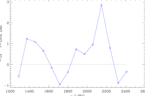
These discrepancies to the generic relations express, in fact, the variety of stars. In each regime, Eqs. (30) and (33) provide a reference for the oscillation pattern, and Eq. (23) indicates the small departure due to the specific interior properties of a star. Asteroseismic inversion could not operate if all oscillation spectra were degenerate and exactly similar to the mean asymptotic spectrum depicted by Eq. (30) and (33)). Conversely, if one assumes that the asymptotic relation provides a reliable reference case for a given stellar model represented by its large separation, then comparing an observed spectrum to the mean spectrum expected at $\Delta\nu$ may provide a way to determine the glitches. In other words, glitches may correspond to observed modulation after subtraction of the mean curvature. We show this in an example (Fig. 9), where we subtracted the mean asymptotic slope derived from Eq. (18) from the local large separations $\nu_{n+1,0}-\nu_{n,0}$.

Figure 9: Variation of the large separation difference $\Delta\nu_{n+1,0}-(\Delta\nu_{n,0})_{\mathrm{as}}$ as a function of $\nu_{n,0}$ for the star HD 49933.

5 Conclusion

We have addressed some consequences of the expected difference between the observed and asymptotic values of the large separation. We derived the curvature of the radial-mode oscillation pattern in a large set of solar-like oscillation spectra from the variation in frequency of the spacings between consecutive radial orders. We then proposed a simple model to represent the observed spectra with the exact asymptotic form. Despite the spread of the data, the ability of the Tassoul asymptotic expansion to account for the solar-like oscillation spectra is confirmed, since we have demonstrated coherence between the observed and asymptotic parameters. Two regimes have been identified: one corresponds to the subgiants and main-sequence stars, the other to red giants. These regimes explain the variation of the observed offset $\varepsilon_{\mathrm{obs}}$ with the large separation.

Curvature and second-order effect:

We have verified that the curvature observed in the échelle diagram of solar-like oscillation spectra corresponds to the second-order term of the Tassoul equation. We have shown that the curvature scales approximately as $(\Delta\nu/\nu_{\mathrm{max}})^{2}$ for subgiants and main-sequence stars. Its behavior changes in the red giant regime, where it varies approximately as $(\Delta\nu/\nu_{\mathrm{max}})$ for red giants.

Large separation and scaling relations:

As the ratio $\Delta\nu_{\mathrm{as}}/\Delta\nu_{\mathrm{obs}}$ changes along the stellar evolution (from about 2 % for a low-mass dwarf to 4 % for a giant), scaling relations must be corrected to avoid a systematic overestimate of the seismic proxies. Corrections are proposed for the stellar radius and mass, which avoid a bias of 2.5 % for $R$ and 5 % for $M$. The corrected and calibrated scaling relations then provide an estimate of $R$ and $M$ with 1-$\sigma$ uncertainties of, respectively, 4 and 8 % for low-mass stars.

Offsets:

The observed values $\varepsilon_{\mathrm{obs}}$ are affected by the definition and the measurement of the large separation. Their spread is amplified by all glitches affecting solar-like oscillation spectra. We made clear that the variation of $\varepsilon_{\mathrm{obs}}$ with stellar evolution is mainly an artefact due to the use of $\Delta\nu_{\mathrm{obs}}$ instead of $\Delta\nu_{\mathrm{as}}$ in the asymptotic relation. This work shows that the asymptotic value $\varepsilon_{\mathrm{as}}$ is a small constant which does vary much throughout stellar evolution for low-mass stars and red giants. It is very close to the value 1/4 derived from the asymptotic expansion for low-mass stars.

Generic asymptotic relation:

According to this, we have established a generic form of the asymptotic relation of radial modes in low-mass stars. The mean oscillation pattern based on this relation can serve as a reference for rapidly analyzing a large amount of data, for identifying unambiguously an oscillation pattern, and for determining acoustic glitches. Departure from the generic asymptotic relation is expected for main-sequence stars with a convective core and for red giants, according to the asymptotic expansion of structure discontinuities.

Last but not least, this work implies that all the quantitative conclusions of previous analyses that have created confusion between $\Delta\nu_{\mathrm{as}}$ and $\Delta\nu_{\mathrm{obs}}$ have to be reconsidered. The observed values derived from the oscillation spectra have to be translated into asymptotic values before any physical analysis. To avoid confusion, it is also necessary to specify which value of the large separation is considered. A coherent notation for the observed value of the large separation at $\nu_{\mathrm{max}}$ should be $\Delta\nu_{\mathrm{max}}$.

Table 2: Stellar parameters

Star(a)	$n_{\mathrm{max}}$	$\Delta\nu_{\mathrm{obs}}$	$\Delta\nu_{\mathrm{as}}^{(b)}$	$\nu_{\mathrm{max}}$	$\varepsilon_{\mathrm{obs}}$	$\alpha_{\mathrm{obs}}$	$T_{\mathrm{eff}}^{(c)}$	$M_{\mathrm{mod}}^{(d)}$	$M^{(e)}$	$R_{\mathrm{mod}}^{(d)}$	$R^{(e)}$	Ref.(f)
		($\mu$Hz)	($\mu$Hz)	($\mu$Hz)		$\times 10^{3}$	(K)	$(M_{\odot})$	$(M_{\odot})$	$(R_{\odot})$	$(R_{\odot})$
HD 181907	8.2	3.41	3.55	28.0	1.08	10.2	4790	1.20	1.29	12.20	12.6	2010Car, 2010Mig
KIC 4044238	8.3	4.07	4.23	33.7	0.94	6.5	4800		1.11		10.6	2012Mos
HD 50890	8.8	1.71	1.78	15.0	0.81	8.6	4670	4.20	3.03	29.90	26.4	2012Bau
KIC 5000307	9.1	4.74	4.93	43.2	0.98	9.9	4992		1.35		10.2	2012Mos
KIC 9332840	9.4	4.39	4.57	41.4	0.94	10.3	4847		1.55		11.3	2012Mos
KIC 4770846	9.8	5.48	5.70	53.9	0.98	9.7	4801		1.39		9.37	2012Mo2
KIC 2013502	10.7	5.72	5.95	61.2	1.01	6.1	4835		1.73		9.80	2012Mos
KIC 10866415	10.8	8.75	9.10	94.4	1.19	8.5	4812		1.15		6.44	2012Mo2
KIC 11550492	10.9	8.70	9.05	94.4	1.13	7.3	4723		1.14		6.46	2012Mo2
KIC 9574650	10.9	9.64	10.03	105	1.16	6.1	5015		1.16		6.06	2012Mo2
KIC 3744043	11.2	9.90	10.30	111	1.18	9.0	4994		1.21		6.03	2012Mos
KIC 9267654	11.4	10.4	10.8	117	1.18	6.7	4965		1.19		5.83	2012Mo2
KIC 6144777	11.6	11.0	11.5	128	1.20	7.8	4657		1.09		5.42	2012Mo2
KIC 5858947	11.7	14.5	15.1	169	1.28	4.0	4977		0.92		4.27	2012Mo2
KIC 6928997	11.9	10.1	10.5	120	1.17	6.4	4800		1.35		6.20	2011Bec, 2012Mos
KIC 11618103	12.3	9.38	9.76	115	1.15	10.0	4870	1.45	1.60	6.60	6.87	2011Jia
KIC 8378462	12.4	7.27	7.56	90.3	1.10	8.5	4962		2.21		9.06	2012Mos
KIC 12008916	12.4	12.9	13.4	159	1.24	6.7	4830	1.26	1.21	5.18	5.07	2012Bec
KIC 9882316	13.1	13.7	14.2	179	1.28	6.4	5228		1.49		5.22	2012Mos
KIC 5356201	13.2	15.8	16.5	209	1.30	8.6	4840	1.23	1.19	4.47	4.38	2012Bec
KIC 8366239	13.3	13.7	14.2	182	1.28	4.8	4980	1.49	1.46	5.30	5.18	2012Bec
KIC 7341231	13.8	28.8	30.0	399	1.33	6.7	5300	0.83	0.85	2.62	2.63	2012Deh
KIC 11717120	14.9	37.3	38.8	555	1.50	6.4	5150		0.78		2.15	2012App, 2012Bru
KIC 9574283	15.1	29.7	30.9	448	1.46	6.5	5440		1.11		2.82	2012App
KIC 8026226	15.2	34.3	35.6	520	1.50	4.0	6230		1.21		2.64	2012App, 2012Bru
KIC 5607242	15.3	39.8	41.4	610	1.43	5.0	5680		0.93		2.18	2012App
KIC 8702606	15.8	39.7	41.2	626	1.36	3.6	5540		0.99		2.23	2012App, 2012Bru
KIC 4351319	15.8	24.4	25.4	387	1.47	4.1	4700	1.30	1.27	3.40	3.36	2011diM
KIC 11771760	16.0	31.7	32.9	505	1.54	6.9	6030		1.46		2.96	2012App
KIC 7976303	16.2	51.1	53.0	826	1.27	4.0	6260		1.00		1.90	2012App
HD 182736	16.4	34.6	35.9	568	1.44	2.8	5261	1.30	1.19	2.70	2.61	2012Hub
KIC 10909629	16.5	49.2	51.0	813	1.28	3.5	6490		1.17		2.05	2012App
KIC 11414712	16.7	43.6	45.2	730	1.43	5.4	5635		1.11		2.19	2012App, 2012Bru
KIC 5955122	16.8	49.1	50.9	826	1.39	4.6	5837		1.06		1.99	2012App, 2012Bru
KIC 7799349	16.9	33.1	34.2	560	1.55	5.9	5115		1.31		2.78	2012App, 2012Bru
Procyon	17.0	54.1	56.0	918	1.41	3.2	6550	1.46	1.17	2.04	1.93	2010Bed, 2008Mos
KIC 1435467	17.4	79.6	82.4	1384	1.30	3.6	6570		0.86		1.35	2012App, 2012Bru
KIC 12508433	17.5	44.8	46.3	784	1.49	5.4	5280		1.13		2.16	2012App
KIC 11193681	17.6	42.7	44.2	752	1.40	4.8	5690		1.35		2.37	2012App
KIC 11395018	17.6	47.4	49.0	834	1.46	3.5	5650	1.35	1.20	2.21	2.13	2011Mat, 2012Cre
KIC 11026764	17.6	50.3	52.0	885	1.39	4.9	5682		1.14		2.01	2011Cam, 2012App, 2012Bru
HD 49385	17.9	55.5	57.4	994	1.39	5.6	6095	1.25	1.21	1.94	1.92	2010Deh, 2011Deh
KIC 11713510	17.9	68.9	71.3	1235	1.42	2.9	5930	1.00	0.94	1.57	1.53	2012Mat
KIC 10920273	17.9	57.2	59.2	1026	1.41	4.6	5880	1.23	1.12	1.88	1.83	2011Cam, 2012Cre
KIC 10018963	17.9	55.1	56.9	988	1.20	4.9	6020		1.21		1.93	2012App, 2012Bru
KIC 3632418	17.9	60.4	62.4	1084	1.19	3.2	6190	1.40	1.15	1.91	1.78	2012App, 2012Sil, 2012Bru
KIC 10162436	18.1	55.5	57.3	1004	1.18	4.3	6200	1.36	1.28	2.01	1.96	2012App, 2012Sil, 2012Bru
KIC 8524425	18.1	59.4	61.4	1078	1.49	5.2	5634		1.05		1.75	2012App, 2012Bru
KIC 7747078	18.2	53.8	55.5	977	1.30	4.0	5840	1.13	1.23	1.95	1.97	2012App, 2012Sil, 2012Bru
KIC 7103006	18.2	58.9	60.8	1072	1.33	5.1	6394		1.30		1.89	2012App, 2012Bru
HD 169392	18.3	56.3	58.1	1030	1.17	2.9	5850	1.15	1.20	1.88	1.90	2012Ma2
KIC 9812850	18.4	64.5	66.6	1186	1.13	2.1	6325		1.20		1.73	2012App, 2012Bru
KIC 12317678	18.4	63.1	65.1	1162	1.47	5.4	6540		1.30		1.80	2012App
KIC 8694723	18.6	74.3	76.7	1384	1.29	4.2	6120		1.03		1.50	2012App, 2012Bru
KIC 8228742	18.7	61.8	63.8	1153	1.25	2.3	6042	1.38	1.22	1.85	1.79	2012App, 2012Sil, 2012Bru
KIC 10273246	18.7	48.8	50.4	913	1.10	3.3	6150	1.37	1.60	2.19	2.30	2011Cam, 2012Cre
KIC 6933899	19.0	71.8	74.1	1362	1.42	3.0	5860		1.06		1.55	2012App, 2012Bru
KIC 11244118	19.0	71.2	73.4	1352	1.44	3.4	5745		1.04		1.55	2012App, 2012Bru
HD 179070	19.0	60.6	62.6	1153	1.14	2.6	6131	1.34	1.35	1.86	1.88	2012How
KIC 9410862	19.3	105.6	108.9	2034	1.53	3.1	6180		0.82		1.10	2012App
KIC 10355856	19.4	67.0	69.1	1303	1.10	3.8	6350		1.38		1.77	2012App, 2012Bru
KIC 12258514	19.4	74.5	76.8	1449	1.36	2.0	5930	1.30	1.12	1.63	1.54	2012App, 2012Sil, 2012Bru
KIC 7206837	19.7	78.9	81.3	1556	1.14	2.1	6384		1.24		1.53	2012App, 2012Bru
KIC 10516096	20.0	84.4	86.9	1689	1.33	2.0	5940	1.12	1.09	1.42	1.40	2012Mat, 2012Bru
KIC 7680114	20.1	84.9	87.4	1705	1.42	3.4	5855	1.19	1.07	1.45	1.39	2012Mat, 2012Bru
KIC 12009504	20.1	87.8	90.4	1768	1.32	2.4	6065		1.10		1.37	2012App, 2012Bru
KIC 6116048	20.2	100.2	103.2	2020	1.44	2.7	5935		0.93		1.19	2012App, 2012Bru
KIC 8760414	20.2	116.4	119.9	2349	1.53	2.7	5787	0.81	0.78	1.02	1.01	2012Mat, 2012App, 2012Bru
KIC 10963065	20.2	102.6	105.6	2071	1.41	2.9	6060		0.95		1.18	2012App, 2012Bru
KIC 3656476	20.4	93.3	96.1	1904	1.41	3.4	5710	1.09	0.98	1.32	1.27	2012Mat, 2012Bru
KIC 11081729	20.4	89.0	91.6	1820	1.26	3.5	6630		1.30		1.44	2012App, 2012Bru
HD 46375	20.5	154.0	158.5	3150	1.50	2.6	5300		0.54		0.74	2010Gau
KIC 9139163	20.5	80.3	82.6	1649	1.06	3.5	6400	1.40	1.38	1.57	1.57	2012App, 2012Sil, 2012Bru
KIC 9098294	20.6	108.7	111.9	2241	1.47	2.5	5840		0.90		1.11	2012App, 2012Bru
KIC 4914923	20.8	88.7	91.2	1848	1.34	2.6	5905	1.10	1.16	1.37	1.39	2012Mat, 2012Bru
HD 181420	21.0	74.9	77.1	1573	0.98	3.7	6580	1.58	1.65	1.69	1.75	2009Bar, 2012Oze
HD 49933	21.0	85.8	88.3	1805	1.04	2.4	6780	1.30	1.52	1.41	1.55	2009Ben, 2012Ree
KIC 6603624	21.1	109.8	112.9	2312	1.56	2.6	5625	1.01	0.90	1.15	1.11	2012Mat, 2012App, 2012Bru
16 Cyg A	21.3	102.5	105.4	2180	1.46	2.9	5825	1.11	1.05	1.24	1.22	2012Met
KIC 8394589	21.4	108.9	112.0	2336	1.37	3.0	6114		1.09		1.19	2012App, 2012Bru
KIC 11253226	21.8	77.0	79.1	1678	0.96	2.3	6605	1.46	1.82	1.63	1.77	2012App, 2012Sil, 2012Bru
$\mu$Arae	21.8	89.5	91.9	1950	1.46	2.4	5813	1.14	1.29	1.36	1.43	2005Bou, 2005Baz
HD 52265	21.8	98.5	101.2	2150	1.38	1.8	6100	1.27	1.27	1.34	1.34	2011Bal, 2012Giz
KIC 6106415	21.9	103.9	106.7	2274	1.38	3.0	5990	1.12	1.18	1.24	1.26	2012Mat, 2012Bru
KIC 10454113	22.1	104.7	107.6	2313	1.27	2.8	6120	1.16	1.24	1.25	1.27	2012App, 2012Sil, 2012Bru
KIC 8379927	22.2	120.0	123.3	2669	1.37	2.4	5990		1.07		1.11	2012App
KIC 9139151	22.3	116.9	120.1	2610	1.40	2.1	6125	1.22	1.15	1.18	1.15	2012App, 2012Sil, 2012Bru
16 Cyg B	22.4	115.3	118.4	2578	1.48	2.8	5750	1.07	1.07	1.13	1.14	2012Met
KIC 9025370	22.4	132.3	135.9	2964	1.48	1.8	5660		0.91		0.98	2012App
KIC 3427720	22.4	119.3	122.5	2674	1.48	3.1	6040		1.12		1.13	2012App, 2012Bru
KIC 5184732	22.5	95.3	97.9	2142	1.43	3.3	5840	1.25	1.34	1.36	1.39	2012Mat, 2012Bru
Sun	22.7	134.4	138.0	3050	1.51	2.0	5777	1.00	0.97	1.00	0.99	Sun
KIC 8379927	22.8	120.4	123.6	2743	1.29	2.2	5900	1.09	1.13	1.11	1.12	2012Mat, 2012App
$\alpha$ Cen A	22.8	105.7	108.5	2410	1.36	1.7	5790	1.10	1.25	1.23	1.27	2004Bed, 2002The
KIC 8006161	23.2	148.5	152.3	3444	1.68	2.2	5390	1.00	0.84	0.93	0.89	2012Mat, 2012App, 2012Bru
18 Sco	23.2	133.5	136.9	3100	1.54	1.8	5813	1.02	1.06	1.01	1.03	2011Baz, 2012Baz
KIC 10644253	23.3	123.0	126.2	2866	1.47	2.6	6030		1.22		1.14	2012App, 2012Bru
KIC 11772920	23.4	155.3	159.3	3639	1.52	1.8	5420		0.84		0.86	2012App
KIC 9955598	23.5	152.6	156.5	3579	1.58	2.1	5410		0.85		0.88	2012App, 2012Bru
$\alpha$ Cen B	25.3	161.4	165.3	4090	1.48	1.6	5260	0.91	0.98	0.86	0.88	2005Kje, 2002The

Table 2: continued.

(a) Stars are sorted by increasing $n_{\mathrm{max}}$ values.
(b) $\Delta\nu_{\mathrm{as}}$ is derived from this work.
(c) $T_{\mathrm{eff}}$ provided by Bruntt et al. (2012), when available.
(d) $M_{\mathrm{mod}}$ and $R_{\mathrm{mod}}$ were obtained from modeling or from interferometry, not from seismic scaling relations.
(e) $M$ and $R$ are derived from the scaling relations Eqs. (28) and (29) with the new calibrations defined by this work.
(f) References are defined by:
2002The = Thévenin et al. (2002)
2004Bed = Bedding et al. (2004)
2005Baz = Bazot et al. (2005)
2005Bou = Bouchy et al. (2005)
2005Kje = Kjeldsen et al. (2005)
2006Cat = Catala et al. (2006)
2008Mos = Mosser et al. (2008a)
2009Bar = Barban et al. (2009)
2009Ben = Benomar et al. (2009)
2010Bed = Bedding et al. (2010b)
2010Car = Carrier et al. (2010)
2010Deh = Deheuvels et al. (2010)
2010Gau = Gaulme et al. (2010)
2010Mig = Miglio et al. (2010)
2011Bal = Ballot et al. (2011)
2011Baz = Bazot et al. (2011)
2011Bec = Beck et al. (2011)
2011Cam = Campante et al. (2011)
2011Deh = Deheuvels & Michel (2011)
2011diM = di Mauro et al. (2011)
2011Jia = Jiang et al. (2011)
2011Mat = Mathur et al. (2011)
2012App = Appourchaux et al. (2012)
2012Bau = Baudin et al. (2012)
2012Baz = Bazot et al. (2012)
2012Bec = Beck et al. (2012)
2012Bru = Bruntt et al. (2012)
2012Cre = Creevey et al. (2012)
2012Deh = Deheuvels et al. (2012)
2012Giz = Gizon et al. (2012)
2012How = Howell et al. (2012)
2012Hub = Huber et al. (2012)
2012Mat = Mathur et al. (2012)
2012Ma2 = Mathur et al. (2013)
2012Met = Metcalfe et al. (2012)
2012Mos = Mosser et al. (2012c)
2012Mo2 = Mosser et al. (2012b)
2012Oze = Ozel et al. (2012)
2012Ree = Reese et al. (2012)
2012Sil = Silva Aguirre et al. (2012)

References

- Appourchaux et al. (2012) Appourchaux, T., Chaplin, W. J., García, R. A., et al. 2012, A&A, 543, A54
- Appourchaux et al. (2008) Appourchaux, T., Michel, E., Auvergne, M., et al. 2008, A&A, 488, 705
- Audard & Provost (1994) Audard, N. & Provost, J. 1994, A&A, 282, 73
- Ballot et al. (2011) Ballot, J., Gizon, L., Samadi, R., et al. 2011, A&A, 530, A97
- Barban et al. (2009) Barban, C., Deheuvels, S., Baudin, F., et al. 2009, A&A, 506, 51
- Baudin et al. (2012) Baudin, F., Barban, C., Goupil, M. J., et al. 2012, A&A, 538, A73
- Bazot et al. (2012) Bazot, M., Campante, T. L., Chaplin, W. J., et al. 2012, A&A, 544, A106
- Bazot et al. (2011) Bazot, M., Ireland, M. J., Huber, D., et al. 2011, A&A, 526, L4
- Bazot et al. (2005) Bazot, M., Vauclair, S., Bouchy, F., & Santos, N. C. 2005, A&A, 440, 615
- Beck et al. (2011) Beck, P. G., Bedding, T. R., Mosser, B., et al. 2011, Science, 332, 205
- Beck et al. (2012) Beck, P. G., Montalban, J., Kallinger, T., et al. 2012, Nature, 481, 55
- Bedding et al. (2001) Bedding, T. R., Butler, R. P., Kjeldsen, H., et al. 2001, ApJ, 549, L105
- Bedding et al. (2010a) Bedding, T. R., Huber, D., Stello, D., et al. 2010a, ApJ, 713, L176
- Bedding et al. (2004) Bedding, T. R., Kjeldsen, H., Butler, R. P., et al. 2004, ApJ, 614, 380
- Bedding et al. (2010b) Bedding, T. R., Kjeldsen, H., Campante, T. L., et al. 2010b, ApJ, 713, 935
- Belkacem et al. (2011) Belkacem, K., Goupil, M. J., Dupret, M. A., et al. 2011, A&A, 530, A142
- Benomar et al. (2009) Benomar, O., Baudin, F., Campante, T. L., et al. 2009, A&A, 507, L13
- Bouchy et al. (2005) Bouchy, F., Bazot, M., Santos, N. C., Vauclair, S., & Sosnowska, D. 2005, A&A, 440, 609
- Bruntt et al. (2012) Bruntt, H., Basu, S., Smalley, B., et al. 2012, MNRAS, 423, 122
- Campante et al. (2011) Campante, T. L., Handberg, R., Mathur, S., et al. 2011, A&A, 534, A6
- Carrier et al. (2010) Carrier, F., De Ridder, J., Baudin, F., et al. 2010, A&A, 509, A73
- Catala et al. (2006) Catala, C., Forveille, T., & Lai, O. 2006, AJ, 132, 2318
- Christensen-Dalsgaard & Frandsen (1983) Christensen-Dalsgaard, J. & Frandsen, S. 1983, Sol. Phys., 82, 469
- Christensen-Dalsgaard & Perez Hernandez (1992) Christensen-Dalsgaard, J. & Perez Hernandez, F. 1992, MNRAS, 257, 62
- Corsaro et al. (2012) Corsaro, E., Stello, D., Huber, D., et al. 2012, ApJ, 757, 190
- Creevey et al. (2012) Creevey, O. L., Doğan, G., Frasca, A., et al. 2012, A&A, 537, A111
- De Ridder et al. (2009) De Ridder, J., Barban, C., Baudin, F., et al. 2009, Nature, 459, 398
- Deheuvels et al. (2010) Deheuvels, S., Bruntt, H., Michel, E., et al. 2010, A&A, 515, A87
- Deheuvels et al. (2012) Deheuvels, S., García, R. A., Chaplin, W. J., et al. 2012, ApJ, 756, 19
- Deheuvels & Michel (2011) Deheuvels, S. & Michel, E. 2011, A&A, 535, A91
- di Mauro et al. (2011) di Mauro, M. P., Cardini, D., Catanzaro, G., et al. 2011, MNRAS, 415, 3783
- Eddington (1917) Eddington, A. S. 1917, The Observatory, 40, 290
- Gaulme et al. (2010) Gaulme, P., Deheuvels, S., Weiss, W. W., et al. 2010, A&A, 524, A47
- Grec et al. (1983) Grec, G., Fossat, E., & Pomerantz, M. A. 1983, Sol. Phys., 82, 55
- Hekker et al. (2011) Hekker, S., Elsworth, Y., De Ridder, J., et al. 2011, A&A, 525, A131
- Hekker et al. (2012) Hekker, S., Elsworth, Y., Mosser, B., et al. 2012, A&A, 544, A90
- Hekker et al. (2009) Hekker, S., Kallinger, T., Baudin, F., et al. 2009, A&A, 506, 465
- Howell et al. (2012) Howell, S. B., Rowe, J. F., Bryson, S. T., et al. 2012, ApJ, 746, 123
- Huber et al. (2011) Huber, D., Bedding, T. R., Stello, D., et al. 2011, ApJ, 743, 143
- Huber et al. (2010) Huber, D., Bedding, T. R., Stello, D., et al. 2010, ApJ, 723, 1607
- Huber et al. (2012) Huber, D., Ireland, M. J., Bedding, T. R., et al. 2012, ApJ, 760, 32
- Jiang et al. (2011) Jiang, C., Jiang, B. W., Christensen-Dalsgaard, J., et al. 2011, ApJ, 742, 120
- Kallinger et al. (2012) Kallinger, T., Hekker, S., Mosser, B., et al. 2012, A&A, 541, A51
- Kallinger et al. (2010) Kallinger, T., Mosser, B., Hekker, S., et al. 2010, A&A, 522, A1
- Kjeldsen et al. (2005) Kjeldsen, H., Bedding, T. R., Butler, R. P., et al. 2005, ApJ, 635, 1281
- Mathur et al. (2013) Mathur, S., Bruntt, H., Catala, C., et al. 2013, A&A, 549, A12
- Mathur et al. (2011) Mathur, S., Handberg, R., Campante, T. L., et al. 2011, ApJ, 733, 95
- Mathur et al. (2012) Mathur, S., Metcalfe, T. S., Woitaszek, M., et al. 2012, ApJ, 749, 152
- Mazumdar et al. (2012) Mazumdar, A., Michel, E., Antia, H. M., & Deheuvels, S. 2012, A&A, 540, A31
- Metcalfe et al. (2012) Metcalfe, T. S., Chaplin, W. J., Appourchaux, T., et al. 2012, ApJ, 748, L10
- Michel et al. (2008) Michel, E., Baglin, A., Auvergne, M., et al. 2008, Science, 322, 558
- Miglio et al. (2012) Miglio, A., Brogaard, K., Stello, D., et al. 2012, MNRAS, 419, 2077
- Miglio et al. (2009) Miglio, A., Montalbán, J., Baudin, F., et al. 2009, A&A, 503, L21
- Miglio et al. (2010) Miglio, A., Montalbán, J., Carrier, F., et al. 2010, A&A, 520, L6
- Mosser & Appourchaux (2009) Mosser, B. & Appourchaux, T. 2009, A&A, 508, 877
- Mosser et al. (2011) Mosser, B., Belkacem, K., Goupil, M., et al. 2011, A&A, 525, L9
- Mosser et al. (2010) Mosser, B., Belkacem, K., Goupil, M., et al. 2010, A&A, 517, A22
- Mosser et al. (2008a) Mosser, B., Bouchy, F., Martić, M., et al. 2008a, A&A, 478, 197
- Mosser et al. (2008b) Mosser, B., Deheuvels, S., Michel, E., et al. 2008b, A&A, 488, 635
- Mosser et al. (2012a) Mosser, B., Elsworth, Y., Hekker, S., et al. 2012a, A&A, 537, A30
- Mosser et al. (1991) Mosser, B., Gautier, D., Schmider, F. X., & Delache, P. 1991, A&A, 251, 356
- Mosser et al. (2012b) Mosser, B., Goupil, M. J., Belkacem, K., et al. 2012b, A&A, 548, A10
- Mosser et al. (2012c) Mosser, B., Goupil, M. J., Belkacem, K., et al. 2012c, A&A, 540, A143
- Mosser et al. (1994) Mosser, B., Gudkova, T., & Guillot, T. 1994, A&A, 291, 1019
- Mosser et al. (2009) Mosser, B., Michel, E., Appourchaux, T., et al. 2009, A&A, 506, 33
- Provost et al. (1993) Provost, J., Mosser, B., & Berthomieu, G. 1993, A&A, 274, 595
- Reese et al. (2012) Reese, D. R., Marques, J. P., Goupil, M. J., Thompson, M. J., & Deheuvels, S. 2012, A&A, 539, A63
- Roxburgh & Vorontsov (2000) Roxburgh, I. W. & Vorontsov, S. V. 2000, MNRAS, 317, 141
- Roxburgh & Vorontsov (2001) Roxburgh, I. W. & Vorontsov, S. V. 2001, MNRAS, 322, 85
- Scherrer et al. (1983) Scherrer, P. H., Wilcox, J. M., Christensen-Dalsgaard, J., & Gough, D. O. 1983, Sol. Phys., 82, 75
- Silva Aguirre et al. (2012) Silva Aguirre, V., Casagrande, L., Basu, S., et al. 2012, ApJ, 757, 99
- Stello et al. (2010) Stello, D., Basu, S., Bruntt, H., et al. 2010, ApJ, 713, L182
- Stello et al. (2011) Stello, D., Huber, D., Kallinger, T., et al. 2011, ApJ, 737, L10
- Tassoul (1980) Tassoul, M. 1980, ApJS, 43, 469
- Thévenin et al. (2002) Thévenin, F., Provost, J., Morel, P., et al. 2002, A&A, 392, L9
- Verner et al. (2011) Verner, G. A., Elsworth, Y., Chaplin, W. J., et al. 2011, MNRAS, 415, 3539
- White et al. (2012) White, T. R., Bedding, T. R., Gruberbauer, M., et al. 2012, ApJ, 751, L36
- White et al. (2011) White, T. R., Bedding, T. R., Stello, D., et al. 2011, ApJ, 743, 161