Parity-time symmetric optical coupler with birefringent arms

Abstract

In this work, we propose a parity-time (${\cal PT}$-) symmetric optical coupler whose arms are birefringent waveguides as a realistic physical model which leads to a so-called quadrimer i.e., a four complex field setting. We seek stationary solutions of the resulting linear and nonlinear model, identifying its linear point of ${\cal PT}$ symmetry breaking and examining the corresponding nonlinear solutions that persist up to this point, as well as, so-called, ghost states that bifurcate from them. We obtain the relevant symmetry breaking bifurcations between symmetric (circularly polarized) and asymmetric (elliptically polarized) states and numerically follow the associated dynamics which give rise to growth/decay even within the ${\cal PT}$-symmetric phase. Our symmetric stationary nonlinear solutions are found to terminate in saddle-center bifurcations which are analogous to the linear ${\cal PT}$-phase transition. We found that the ${\cal PT}$ symmetry significantly changes the stability and dynamical properties of the modes with different polarizations.

I Introduction

An optical coupler with one arm having losses and another one having gain, balanced against each other, recently became a test-bed for many phenomena originating from the interplay of the parity-time (${\cal PT}$) symmetry and nonlinearity. Unidirectional dynamics kot1 , unversality of the dynamics kot2 , symmetry breaking properties kip ; pgk , switching of the beams sukh1 and of solitons R30add3 , formation of symmetric and asymmetric bright solitary waves R30add1 ; R30add2 , breathers baras , and their stability R30add4 , dark solitons BKM , as well as the emergence of ghost states R46a ; R46b ; R46 and large-scale temporal ${\cal PT}$-symmetric lattices christo_nat2 are some among the many topics that have been touched upon in very intense recent theoretical and experimental work.

As a direct extension of the previous activity, a large chunk of which has focused on the prototypical setting of the ${\cal PT}$-symmetric dimer, there emerges a problem of effect of ${\cal PT}$ symmetry and nonlinearity on the polarization of the electric field. In that regard, the previously proposed settings, to the best of our knowledge, were chiefly focused on effectively scalar models. On the other hand, the “vector” type of problems is natural for experimental settings where the exploited fibers obey birefringence, since the two orthogonal polarizations are to be taken into account Menyuk .

In this work we consider a ${\cal PT}$-symmetric coupler whose arms are birefringent waveguides. Assuming that the first waveguide is active and the second one is absorbing, we address the problem of a ${\cal PT}$-preserving (in the linear limit) configuration. While being an interesting model from a physical point of view, this setting also offers a different (in comparison to what was studied before) mathematical situation where the nonlinear modes bifurcate from doubly degenerated eigenvalues of the linear problem. This requires the generalization of earlier developed approaches (e.g. like the one reported in ZK ) for the bifurcation of the nonlinear modes from the linear spectrum. In addition, it presents a rich playground for dynamical systems analysis, due to the emergence of a variety of saddle-center bifurcations (nonlinear analogs of the linear ${\cal PT}$-phase transition), as well as symmetry-breaking (pitchfork) ones. It is these nonlinear states, their emergence, stability, dynamics and the asymptotics of the system that we will focus on hereafter.

The organization of the paper is as follows. In section II, we present the model in its evolution as well as in its stationary form. In section III, we focus on its linear properties. Then, in section IV, we examine the nonlinear modes (and bifurcations). Finally, in section V, we briefly touch upon the dynamical implications of our findings and in section VI, we present some conclusions, as well as some potential directions for future work.

II The model

We specify the problem by imposing that the principal optical axes of the two Kerr-type waveguides are $\pi/4$-rotated with respect to each other, as it is schematically represented in Fig. 1. In each arm, labeled by $j$, there are two orthogonal field components of the electric fields which we write down in the form Menyuk ($j=1,2$):

$${\bf E}_{j}({\bf r},z,t)=\left[u_{j}(z)A_{j}({\bf r}-{\bf r}_{j})e^{-i\beta_{j}z}{\bf e}_{j}\right.$$

$$+\left.u_{j+2}(z)A_{j+2}({\bf r}-{\bf r}_{j})e^{-i\beta_{j+2}z}{\bf e}_{j+2}\right]\sqrt{\frac{2}{\chi}}e^{i\omega t}+c.c.$$ (1)

Here $u_{j}$ are the field envelopes depending on the propagation distance $z$, i.e. we consider the stationary – in time – problem, assuming that the carrier wavelength $\lambda_{0}$ is in the region of the normal group velocity dispersion, thus ruling out a possibility of modulational instability; ${\bf r}=(x,y)$ is a transverse radius vector, and ${\bf r}_{1,2}$ are the positions of the centers of the cores of the coupler. The real parameters $\beta_{j}$ are the propagation constants of each of the field components, and ${\bf e}_{j}$ are the polarization vectors, which are mutually orthogonal in each arm of the coupler, i.e. ${\bf e}_{1}\cdot{\bf e}_{3}={\bf e}_{2}\cdot{\bf e}_{4}=0$. The real functions $A_{j}({\bf r}-{\bf r}_{j})$ and $A_{j+2}({\bf r}-{\bf r}_{j})$ describe the transverse distributions of the fields in each waveguide and the normalization coefficient $\sqrt{2/\chi}$, where $\chi$ is the Kerr coefficient, is introduced for convenience. For $j=1$ and $j=2$ the functions $A_{j}({\bf r})$ are centered in different points ${\bf r}_{j}$. Also, for the sake of simplicity, we consider $A_{j}({\bf r})=A_{j+2}({\bf r})=A({\bf r})$ (for $j=1,2$), such that the integral

$$({\bf e}_{j}\cdot{\bf e}_{j+1})\frac{\int A({\bf r}-{\bf r}_{j})A({\bf r}-{\bf r}_{j+1})d^{2}{\bf r}}{\int A^{2}({\bf r})d^{2}{\bf r}}$$

(the integration is performed over the transverse plane) describes the linear coupling between the respective modes. Since in the configuration shown in Fig. 1 ${\bf e}_{1}\cdot{\bf e}_{2}={\bf e}_{1}\cdot{\bf e}_{4}={\bf e}_{3}\cdot{\bf e}_{4}=-{\bf e}_{3}\cdot{\bf e}_{2}=1/\sqrt{2}$ we use the single linear coupling coefficient $k$ (see also coupling ).

          

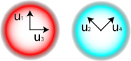
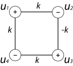
Figure 1: (Color online) (a) Schematic presentation of a ${\cal PT}$-symmetric coupler based on birefringent fibers. (b) Equivalent graph (plaquette) representation illustrating the ${\cal PT}$-symmetry. Here $-$ and $+$ stand for lossy and active waveguides, respectively.

Then following the analysis described in details in Menyuk we end up with the system of equations:

$$i\frac{du_{1}}{dz}=-k(u_{2}+u_{4})+i\gamma u_{1}-\left(|u_{1}|^{2}+\frac{2}{3}|u_{3}|^{2}\right)u_{1}$$

$$-\frac{1}{3}u_{3}^{2}u_{1}^{*}e^{i\Delta_{1}z}$$ (2a)

$$i\frac{du_{2}}{dz}=-k(u_{1}-u_{3})-i\gamma u_{2}-\left(|u_{2}|^{2}+\frac{2}{3}|u_{4}|^{2}\right)u_{2}$$

$$-\frac{1}{3}u_{4}^{2}u_{2}^{*}e^{i\Delta_{2}z}$$ (2b)

$$i\frac{du_{3}}{dz}=-k(u_{4}-u_{2})+i\gamma u_{3}-\left(\frac{2}{3}|u_{1}|^{2}+|u_{3}|^{2}\right)u_{3}$$

$$-\frac{1}{3}u_{1}^{2}u_{3}^{*}e^{-i\Delta_{1}z}$$ (2c)

$$i\frac{du_{4}}{dz}=-k(u_{1}+u_{3})-i\gamma u_{4}-\left(\frac{2}{3}|u_{2}|^{2}+|u_{4}|^{2}\right)u_{4}$$

$$-\frac{1}{3}u_{2}^{2}u_{4}^{*}e^{-i\Delta_{2}z}$$ (2d)

Here $\gamma>0$ describes gain in the first waveguide and dissipation in the second waveguide, $\Delta_{j}=\frac{4\pi c}{\lambda_{0}}\left(\beta_{j}^{\prime}-\beta_{j+2}^{\prime}\right)$ with $\beta_{j}^{\prime}=\frac{d\beta_{j}(\omega_{0})}{d\omega_{0}}$, $\omega_{0}$ being the carrier wave frequency, is a properly normalized mismatch between the propagation constants of the orthogonal polarizations $u_{j+2}$ and $u_{j}$. The asterisk stands for complex conjugation.

We will be interested in the stationary solutions, in particular in their linear stability properties and ensuing nonlinear dynamics which can be found in the two prototypical limiting cases of (i) zero mismatches $|\beta_{j}-\beta_{j+2}|=0$ and (ii) large mismatches $|\beta_{j}^{\prime}-\beta_{j+2}^{\prime}|\gg k\lambda_{0}/c$ when the respective nonlinear terms can be neglected. It is convenient to introduce a parameter $\alpha$ which vanishes ($\alpha=0$) in the case (ii) and is unity ($\alpha=1$) in the case (i). Using the standing wave ansatz $u_{j}(z)=w_{j}e^{ibz}$, where $w_{j}$ are $z-$independent, we obtain the system of algebraic equations:

$$bw_{1}=k(w_{2}+w_{4})-i\gamma w_{1}+\left(|w_{1}|^{2}+\frac{2}{3}|w_{3}|^{2}\right)w_{1}$$

$$+\frac{\alpha}{3}w_{3}^{2}w_{1}^{*},$$ (3a)

$$bw_{2}=k(w_{1}-w_{3})+i\gamma w_{2}+\left(|w_{2}|^{2}+\frac{2}{3}|w_{4}|^{2}\right)w_{2}$$

$$+\frac{\alpha}{3}w_{4}^{2}w_{2}^{*},$$ (3b)

$$bw_{3}=k(w_{4}-w_{2})-i\gamma w_{3}+\left(\frac{2}{3}|w_{1}|^{2}+|w_{3}|^{2}\right)w_{3}$$

$$+\frac{\alpha}{3}w_{1}^{2}w_{3}^{*},$$ (3c)

$$bw_{4}=k(w_{1}+w_{3})+i\gamma w_{4}+\left(\frac{2}{3}|w_{2}|^{2}+|w_{4}|^{2}\right)w_{4}$$

$$+\frac{\alpha}{3}w_{2}^{2}w_{4}^{*}.$$ (3d)

Below the spectral parameter $b$ will be also referred to as the propagation constant.

III Properties of the linear problem

First we address the underlying linear problem [which corresponds to the situation when all cubic terms in Eqs. (3) are negligible]. It can be rewritten in the matrix form $\tilde{b}\tilde{{\bf w}}={H}\tilde{{\bf w}}$ where

$$\tilde{{\bf w}}=\left(\!\!\begin{array}[]{c}\tilde{w}_{1}\\ \tilde{w}_{2}\\ \tilde{w}_{3}\\ \tilde{w}_{4}\end{array}\!\!\right)\,\,\,\mbox{and}\,\,\,{H}=\left(\!\!\begin{array}[]{cccc}-i\gamma&k&0&k\\ k&i\gamma&-k&0\\ 0&-k&-i\gamma&k\\ k&0&k&i\gamma\end{array}\!\right)$$

(hereafter we use tilde in order to distinguish eigenvalues and eigenvectors of the linear problem).

The operator $H$ is ${\cal PT}$ symmetric, which means that $[H,{\cal PT}]=H{\cal PT}-{\cal PT}H=0$, where ${\cal P}$ is a spatial reversal linear operator

$${{\cal P}}=\left(\!\!\begin{array}[]{cccc}0&0&0&1\\ 0&0&1&0\\ 0&1&0&0\\ 1&0&0&0\end{array}\!\right)$$ (9)

and ${\cal T}$ performs element-wise complex conjugation: ${\cal T}{\bf w}={\bf w}^{*}$. The spectrum of operator $H$ consists of two double eigenvalues

$$\tilde{b}_{\pm}=\pm\sqrt{2k^{2}-\gamma^{2}},$$ (10)

which are real for $\gamma<\gamma_{cr}^{(1)}$ where $\gamma_{cr}^{(1)}=\sqrt{2}k$ will be referred to as a primary critical point: the spontaneous ${\cal PT}$ symmetry breaking occurs at $\gamma_{cr}^{(1)}$ above which the eigenvalues are all imaginary. In order to visualize the ${\cal PT}$ symmetry of the linear system, following ZK one can represent it with a graph shown in the right panel of Fig. 1, reminiscent of four linearly coupled waveguides ZK (notice however the sign difference in the coupling constants) or plaquettes guenther .

Since the details of our analysis are the same for both eigenvalues $\tilde{b}_{-}$ and $\tilde{b}_{+}$, we drop the subscripts $+$ and $-$ wherever this does not lead to confusion. Despite having double eigenvalues in its spectrum, $H$ is diagonalizable below the ${\cal PT}$-symmetry breaking point. This means that double eigenvalues are semisimple, i.e. for an eigenvalue $\tilde{b}$ one can find two linearly independent eigenvectors, i.e. $H\tilde{\bf w}^{(j)}=\tilde{b}\tilde{\bf w}^{(j)}$, where $j=1,2$. Moreover, each eigenvalue $\tilde{b}$ possesses an invariant subspace spanned by $\tilde{\bf w}^{(1)}$ and $\tilde{\bf w}^{(2)}$.

Let us also notice the following peculiarity of the case at hand. In a situation where a ${\cal PT}$-symmetric operator $H$ has no multiple eigenvalues, the condition of unbroken ${\cal PT}$ symmetry (i.e. reality of all the eigenvalues) requires that for each eigenvalue $\tilde{b}$ the corresponding eigenvector $\tilde{\bf w}$ can be chosen as an eigenstate of the ${\cal PT}$ operator, i.e. ${\cal PT}\tilde{\bf w}=\tilde{\bf w}$. However, in the situation at hand arbitrarily chosen linearly independent eigenvectors $\tilde{\bf w}^{(1)}$ and $\tilde{\bf w}^{(2)}$ may not be ${\cal PT}$ eigenstates. However, unbroken ${\cal PT}$ symmetry requires that a certain linear combination of $\tilde{\bf w}^{(1)}$ and $\tilde{\bf w}^{(2)}$ is an eigenstate for the ${\cal PT}$ operator. More specifically, it is easy to establish that all the eigenvectors that belong to the invariant subspace of $\tilde{b}$ and, at the same time, are the eigenstates for the ${\cal PT}$ operator, can be parametrized by a complex parameter $a$ as follows:

$$\tilde{\bf w}=\left(\!\!\begin{array}[]{c}a^{*}\\ \frac{ia^{*}(\gamma-i\tilde{b})}{k}-a\\ \frac{-ia(\gamma+i\tilde{b})}{k}-a^{*}\\ a\end{array}\!\right)$$ (11)

Being interested in linearly independent vectors $\tilde{\bf w}$, it is sufficient to consider only the vectors with

$$a=e^{i\theta}.$$ (12)

Then Eq. (11) yields a monoparametric set of eigenvectors $\tilde{\bf w}(\theta)$ with a real parameter $\theta$. In particular, setting $\theta^{(1)}=0$ and $\theta^{(2)}=\arctan(\frac{2k-\tilde{b}}{\gamma})$ one can choose two orthogonal (and therefore linearly independent) eigenvectors:

$$\tilde{\bf w}^{(1,2)}=\tilde{\bf w}(\theta^{(1,2)}),\quad\langle\tilde{\bf w}^{(1)},\tilde{\bf w}^{(2)}\rangle=0$$ (13)

(hereafter we use the standard scalar product $\langle{\bf g},{\bf h}\rangle=\sum_{j=1}^{4}g_{j}h_{j}^{*}$). Any eigenvector $\tilde{\bf w}$ corresponding to the eigenvalue $\tilde{b}$ can be represented as a linear combination of ${\cal PT}$ eigenstates $\tilde{\bf w}^{(1,2)}$: $\tilde{\bf w}=\lambda_{1}\tilde{\bf w}^{(1)}+\lambda_{2}\tilde{\bf w}^{(2)}$ (of course, this does not mean that any eigenvector $\tilde{\bf w}$ is also a ${\cal PT}$ eigenstate).

Let us also introduce a Hermitian adjoint operator $H^{\dagger}$. Since the matrix $H$ is symmetric, one has $H^{\dagger}=H^{*}$. As long as ${\cal PT}$ symmetry of $H$ is unbroken, the spectrum of the adjoint operator $H^{\dagger}$ also consists of two double eigenvalues $b_{\pm}$ which are semi-simple. Any eigenvector corresponding to an eigenvalue $\tilde{b}$ of the adjoint operator $H^{\dagger}$ can be represented as a linear combination of $(\tilde{\bf w}^{(1)})^{*}$ and $(\tilde{\bf w}^{(2)})^{*}$.

IV Nonlinear modes

IV.1 Bifurcations from the linear limit

Now we develop a perturbation theory for the eigenstates of the linear problem giving rise to monoparametric families of nonlinear modes. We will look for nonlinear modes ${\bf w}$ that are eigenstates of the ${\cal PT}$ operator, i.e. ${\cal PT}{\bf w}={\bf w}$. To this end we introduce the expansions

$${\bf w}=\varepsilon\tilde{\bf w}(\theta)+\varepsilon^{3}{{\bf W}}_{3}+\ldots\quad\mbox{and}\quad b=\tilde{b}+\varepsilon^{2}B_{2}+\ldots$$ (14)

Here $\varepsilon$ is a small real parameter, ${\bf W}_{3}$ and $B_{2}$ are the coefficients of the expansions and $\theta$ is to be determined from the symmetry of the solution (see below). We notice that for the expansion to be meaningful the coefficient $B_{2}$ must be real.

Expansions (14) describe nonlinear modes that bifurcate from the linear limit corresponds to $\varepsilon=0$ and is given by the eigenvector $\tilde{\bf w}(\theta)$ being a linear combination of $\tilde{\bf w}^{(1,2)}$ such that ${\cal PT}\tilde{\bf w}(\theta)=\tilde{\bf w}(\theta)$. Respectively, in the linear limit the parameter $b$ is given by the eigenvalue $\tilde{b}$.

Passing from $\varepsilon=0$ to $0<\varepsilon\ll 1$ one has to compute the coefficients ${\bf W}_{3}$ and $B_{2}$. While the physical sense of the coefficient $B_{2}$ is clear — it is a deviation of the propagation constant due to small nonlinearity, it turns out that $B_{2}$ also has a clear geometrical interpretation. Indeed, let us consider the total energy flow through the coupler, which is defined by

$$U=\sum_{j=1}^{4}|w_{j}|^{2},$$ (15)

Expansions (14) imply that in the vicinity of the linear limit $U=\varepsilon^{2}\langle\tilde{\bf w}(\theta),\tilde{\bf w}(\theta)\rangle+O(\varepsilon^{3})$. Therefore, the coefficient $B_{2}$ governs a slope of the energy curve in the vicinity of the bifurcation point, i.e.

$$\left.\frac{\partial U}{\partial b}\right|_{b=\tilde{b},U=0}=\frac{\langle\tilde{\bf w}(\theta),\tilde{\bf w}(\theta)\rangle}{B_{2}}.$$ (16)

For the sake of definiteness, now we concentrate on the case $\alpha=0$. Then the nonlinear problem (3) is conveniently written in the matrix form

$$b{\bf w}=H{\bf w}+F({\bf w}){\bf w},$$ (17)

where $F({\bf w})$ is a diagonal matrix-function describing the nonlinearity: $F({\bf w})=\mbox{diag}(|w_{1}|^{2}+\frac{2}{3}|w_{3}|^{2},|w_{2}|^{2}+\frac{2}{3}|w_{4}|^{2},\frac{2}{3}|w_{1}|^{2}+|w_{3}|^{2},\frac{2}{3}|w_{2}|^{2}+|w_{4}|^{2})$. Substituting (14) into Eq. (17), noticing that $F({\bf w})=\varepsilon^{2}F(\tilde{\bf w})+O(\varepsilon^{3})$, and collecting the terms order of $\varepsilon^{3}$, we obtain

$$(H-\tilde{b}){\bf W}_{3}=-[F(\tilde{\bf w}(\theta))-B_{2}]\tilde{\bf w}(\theta).$$ (18)

Equation (18) implies two possibilities. The first one corresponds to the case when at some $\theta$ the eigenvector $\tilde{\bf w}(\theta)$ of the operator $H$ is simultaneously an eigenvector for the matrix $F(\tilde{\bf w}(\theta))$. Then the coefficient $B_{2}$ can be chosen as an eigenvalue of $F(\tilde{\bf w}(\theta))$ corresponding to the eigenvector $\tilde{\bf w}(\theta)$ (provided that this eigenvalue is real). In this situation, the right hand side of Eq. (18) is zero and it is sufficient to set ${\bf W}_{3}=0$. Since the matrix $F(\tilde{\bf w}(\theta))$ is diagonal, its eigenvalues are equal to its diagonal elements and the corresponding eigenvectors are given as columns of the $4\times 4$ identity matrix.

Let us first assume that all the eigenvalues of $F(\tilde{\bf w}(\theta))$ are simple. In this case $\tilde{\bf w}(\theta)$ can not be an eigenvector for $F(\tilde{\bf w}(\theta))$. The latter fact becomes evident if one notices that $\tilde{\bf w}(\theta)$ has no zero entries for any $\theta$ [see the definition (11)]. Therefore, $\tilde{\bf w}(\theta)$ can be an eigenvector for $F(\tilde{\bf w}(\theta))$ only if $F(\tilde{\bf w}(\theta))$ has a multiple eigenvalue. Then $\tilde{\textbf{w}}(\theta)$ could be searched in the form of a linear combination of eigenvectors corresponding to the multiple eigenvalue. However, using the same argument, i.e. the fact that all entries of the vector $\tilde{\bf w}(\theta)$ are nonzero, one can see that even if $F(\tilde{\bf w}(\theta))$ has a double or an triple eigenvalue, the matrix $F(\tilde{\bf w}(\theta))$ still can not have $\tilde{\bf w}(\theta)$ among its eigenvectors. Therefore $\tilde{\bf w}(\theta)$ can be an eigenvector of $F(\tilde{\bf w}(\theta))$ only if all its eigenvalues are equal. Imposing this constraint on the matrix $F(\tilde{\bf w}(\theta))$, one obtains $|w_{1}|=|w_{3}|$ and $|w_{2}|=|w_{4}|$. Noticing that the form of $\tilde{\textbf{w}}(\theta)$ implies, through Eqs. (11) and (12), that $|w_{1}|=|w_{4}|=1$ we conclude that $\tilde{\bf w}(\theta)$ is an eigenvector of $F(\tilde{\bf w}(\theta))$ only if the moduli of all the entries of $\tilde{\bf w}(\theta)$ are equal to unity. Then matrix $F(\tilde{\bf w}(\theta))$ is equal to the $4\times 4$ identity matrix multiplied by $5/3$. Requiring the moduli of all the entries of $\tilde{\bf w}(\theta)$ to be equal, one arrives at the equation for $\theta$ whose root is given as

$$\theta=\frac{\pi}{8}-\frac{1}{2}\arctan\left(\frac{\tilde{b}}{\gamma}\right).$$ (19)

Since now the moduli of all the entries of $\tilde{\bf w}(\theta)$ are equal to unity and therefore $\langle\tilde{\bf w}(\theta),\tilde{\bf w}(\theta)\rangle=4$, $B_{2}=5/3$ and Eq. (16) readily yields that in the vicinity of $\tilde{b}$ the slope $\left.\partial U/\partial b\right|_{b=\tilde{b},U=0}=12/5=2.4$. Notice that the found value does not depend on $k$ or $\gamma$, and thus these modes correspond to their counterpart in pure conservative coupler with birefringent arms with $\gamma=0$ [Eq. (19) is valid in this case since $\arctan(\pm\infty)=\pm\pi/2$].

Let us now consider the second possibility to fulfill Eq. (18). If for some $\theta$ the corresponding $\tilde{\bf w}(\theta)$ is not an eigenvector for $F(\tilde{\bf w}(\theta))$, then one must satisfy Eq. (18) choosing nonzero ${\bf W}_{3}$. Then the coefficient $B_{2}$ is to be determined from the solvability condition which requires the right hand side of Eq. (18) to be orthogonal to all the eigenvectors of the invariant subspace of $\tilde{b}$ in the spectrum of the adjoint operator $H^{\dagger}$. As we have established in Sec. III, any eigenvector of $H^{\dagger}$ from the invariant subspace of $\tilde{b}$ can be represented as a linear combination of $(\tilde{\bf w}^{(1)})^{*}$ and $(\tilde{\bf w}^{(2)})^{*}$. Requiring the right hand side of Eq. (18) to be orthogonal to an arbitrary linear combination of $(\tilde{\bf w}^{(1)})^{*}$ and $(\tilde{\bf w}^{(2)})^{*}$, we arrive at the following relations:

$$\frac{\langle F(\tilde{\bf w}(\theta))\tilde{\bf w}(\theta),(\tilde{\bf w}^{(1)})^{*}\rangle}{\langle\tilde{\bf w}(\theta),(\tilde{\bf w}^{(1)})^{*}\rangle}=\frac{\langle F(\tilde{\bf w}(\theta))\tilde{\bf w}(\theta),(\tilde{\bf w}^{(2)})^{*}\rangle}{\langle\tilde{\bf w}(\theta),(\tilde{\bf w}^{(2)})^{*}\rangle}=B_{2}.$$ (20)

In Eq. (20) the first equality sign is an equation which is to be solved with respect to $\theta$. Once a root $\theta$ of the latter equation is found, then $B_{2}$ is given from the second equality sign. Notice that despite the fact that the vector $\tilde{\bf w}(\theta)$ is complex, the coefficient $B_{2}$ will be real ZK .

Substituting the expression for $\tilde{\bf w}(\theta)$ into Eq. (20), one obtains a rather cumbersome equation, which, however can be attacked with a computer algebra program. After some transformations, Eq. (20) yields the following condition:

$$|e^{2i\theta}|=\frac{|\gamma-\sqrt{-k^{2}+\gamma^{2}}|}{{k}}.$$ (21)

The latter equation has a real root $\theta$ only if $0<\gamma\leq k$, i.e. when the expression under the radical is not positive. This result suggests that there exists a critical value of the gain-loss parameter which we term as the secondary critical point $\gamma_{cr}^{(2)}=k$, such that for sufficiently small $\gamma$, namely, $0<\gamma\leq\gamma_{cr}^{(2)}$, there exists another family bifurcating from the eigenvalue $\tilde{b}$ of the linear spectrum. However, this family disappears for $\gamma>\gamma_{cr}^{(2)}$, in spite of the fact that the ${\cal PT}$ symmetry of the underlying linear problem remains unbroken, i.e. $\gamma_{cr}^{(2)}<\gamma_{cr}^{(1)}$. It is important to point that the newly found family of solutions does not correspond to equal amplitude among the different nodes, and hence pertains to an elliptically (rather than circularly) polarized family of modes.

Computing the corresponding value of $B_{2}$ for the newly found elliptically polarized family, one finds that the coefficient $B_{2}$ does depend on $k$ and $\gamma$ (in contrast to the above considered circularly polarized family, characterized by $B_{2}=5/3$ for any combination of $k$ and $\gamma$ which does not violate ${\cal PT}$ symmetry). In particular, when $\gamma$ approaches $k$, the coefficient $B_{2}$ of the elliptically polarized family tends to $5/3$, which suggests that at $\gamma=k$ the circularly polarized and elliptically polarized families globally merge.

IV.2 Algebraic analysis and numerical results

IV.2.1 Exact solutions

Having explored nonlinear modes close to the linear limit, where the amplitudes of the modes are small and therefore they can be analyzed by means of perturbation theory, let us now consider nonlinear modes of arbitrary amplitudes (turning again to the general case $\alpha\neq 0$). Relying on results of the previous subsection we firstly search for nonlinear modes which have equal intensities in all four waveguides. Making the substitution $w_{2}=-iw_{1}^{*}$ and imposing the condition $w_{4}=w_{1}^{*}$, $w_{3}=w_{2}^{*}$, which is necessary for a nonlinear mode to be an eigenstate of ${\cal PT}$ thus leading to the circularly polarized light in each of the coupler arms, system (3) yields the single (complex) algebraic equation

$$bw_{1}=k(1-i)w_{1}^{*}+\frac{5-\alpha}{3}|w_{1}|^{2}w_{1}-i\gamma w_{1}.$$ (22)

Representing $w_{1}=\rho e^{i\phi}$, we obtain a bi-quadratic equation for $\rho$ yielding two families of the modes bifurcating from the eigenvalues $\tilde{b}_{\pm}$, given by (10), of the linear spectrum:

$$\rho^{2}_{\pm}=\frac{3(b-\tilde{b}_{\pm})}{5-\alpha},\quad e^{2i\phi_{\pm}}=\frac{\tilde{b}_{\pm}(1-i)-\gamma(1+i)}{2k}.$$ (23)

Respectively, the nonlinear modes have the following form:

$${\bf w}=\left(\!\!\begin{array}[]{c}\rho_{\pm}e^{i\phi_{\pm}}\\ -i\rho_{\pm}e^{-i\phi_{\pm}}\\ i\rho_{\pm}e^{i\phi_{\pm}}\\ \rho_{\pm}e^{-i\phi_{\pm}}\end{array}\!\right)$$ (24)

Using Eqs. (23) one can easily obtain continuous families of nonlinear modes that can be identified as a function of the propagation constant $b$, for given $k$ and $\gamma$.

Let us now recall that Eq. (21) predicts that for $\alpha=0$ and $\gamma<\gamma_{cr}^{(2)}$, there exist families of elliptically polarized modes having different absolute values of the polarization vectors. Such families were indeed found in our numerics. However, all such modes turned out to be unstable (see Figs. 2–3 and discussion below).

In the case of zero propagation constant mismatch, i.e. when $\alpha=1$, one also can find families which have different amplitudes of the polarization vectors. The explicit expressions for the families bifurcating from $\tilde{b}_{\pm}$ read

$$\begin{array}[]{c}w_{1}=w_{4}^{*}=\rho_{\pm}e^{i\phi},w_{2}=w_{3}^{*}=(-1\pm\sqrt{2})\rho_{\pm}e^{-i\phi},\\ \displaystyle{\rho^{2}_{\pm}=\frac{b-\tilde{b}_{\pm}}{4\mp 2\sqrt{2}},\quad\phi=\mp\frac{1}{2}\arcsin\frac{\gamma}{\sqrt{2}k}}.\end{array}$$ (27)

Remarkably, these modes, which also describe propagation of elliptically polarized light, are stable in a certain range of the parameters.

IV.2.2 Families of nonlinear modes

The results of our analysis of the families of nonlinear modes are summarized in Fig. 2. The upper panels show that for $0<\gamma<k$ each eigenvalue of the linearized problem gives rise to two distinct (circularly and elliptically polarized) families of nonlinear modes. In the case of $\alpha=0$ the slopes of the dependencies $U(b)$ are close for the families of both types, and the elliptically polarized families are always unstable while circularly polarized families have both stable and unstable solutions. For $\alpha=1$ one can find stable solutions both for the families with circular and for those with elliptical polarization.

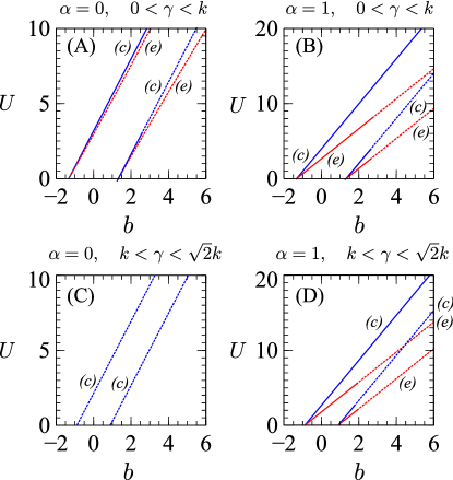
Figure 2: (Color online) Prototypical examples of families of nonlinear modes in the plane $(b,U)$ for $k=1$ and gain-loss parameters $\gamma$: $\gamma=0.5$ (the upper panels), $\gamma=1.1$ (the lower panels). Left and right columns correspond to $\alpha=0$ and $\alpha=1$. Stable and unstable modes are shown by by continuous and broken lines, respectively. The families with the circular and elliptical polarization (if any) are marked with labels “(c)” and “(e)”, respectively (in the color online version families with the circular and elliptical polarization are also shown by blue and red lines, respectively).

For $k<\gamma<\sqrt{2}k$, the case $\alpha=0$ does not allow for elliptically polarized families [see Fig. 2 C], a feature which is in accordance with the perturbation approach developed above. In this case one can only find circularly polarized modes, which are unstable. On the other hand, for $\alpha=1$, stable and unstable modes of both types can be found [see Fig. 2 D].

Summarizing at this point, we have identified 4 sets of solutions, two circularly polarized with equal amplitude at the nodes, and two elliptically polarized with unequal such amplitudes. These all degenerate into the two distinct eigenvalues $\tilde{b}_{\pm}$, given by (10), of the linear problem. The circularly polarized solutions are more robust, while the elliptically polarized ones are always unstable for $\alpha=0$ and stable only for small enough amplitudes for $\alpha=1$. Among the circularly polarized ones, for $0<\gamma<\sqrt{2}k$ the more fundamental state (stemming from the negative eigenvalue at the linear limit) is always the stable ground state of the system in continuations over the parameter $b$, while the excited state is only stable for small enough amplitudes.

IV.2.3 Continuation over $\gamma$

An alternative and perhaps even more telling way to illustrate the above features stems from fixing some value of $b$, starting from the Hamiltonian limit of $\gamma=0$ and subsequently identifying branches of the nonlinear modes by means of changing $\gamma$, as shown in Fig. 3. It is important to note that this alternative viewpoint affords us the ability to visualize bifurcations which we now explore.

The relevant results for parametric continuations over $\gamma$ are given in Figs. 3-4; typical examples of the corresponding linearization spectra for different values of $\gamma$ can be found in Fig. 5. Here, it can be seen that a lower amplitude and a higher-amplitude intensity-symmetric (i.e., equal amplitude) branch exist, for fixed $b$, from the Hamiltonian limit of $\gamma=0$ and all the way up to the linear ${\cal PT}$-phase transition point $\gamma_{cr}^{(1)}=\sqrt{2}k$. At that point, the two equal amplitude branches collide and disappear in a saddle-center bifurcation which can be thought of as a nonlinear analog of the linear ${\cal PT}$-phase transition djf . An additional very interesting feature arises precisely at the point $\gamma_{cr}^{(2)}$ [see (21) and the related discussion], where it can be seen that both branches of equal amplitude between the sites become dynamically unstable for $\alpha=0$. In fact, it is seen that for the larger amplitude branch (associated with the blue circles), one pair of unstable eigenvalues arises, while for the smaller amplitude (red diamond) branch, two such pairs accompany the symmetry breaking bifurcation occurring at this critical point. A closer inspection reveals that the symmetric branch (blue circles) is destabilized through a subcritical pitchfork bifurcation with its “corresponding” asymmetric state (i.e., the one degenerate with it in the linear limit). In the case of the lower amplitude (excited) state for the same $b$, the situation appears to be more complex. In particular, there exists once again a subcritical pitchfork with the corresponding asymmetric branch, yet this would justify one pair of unstable eigenvalues and we observe two. This is because at the same point, there also exists a supercritical pitchfork, which gives rise to the so-called ghost states, denoted by magenta plus symbols. These states are analogous to the ones to analyzed in R46a ; R46b ; R46 , but remarkably are not stationary states of the original problem, yet they are pertinent to its dynamical (instability) evolution and for this reason they will be examined in further detail separately in the dynamics section below.

In the case of $\alpha=1$, only one pair of unstable eigenvalues emerges for the lower amplitude branch at the secondary critical point of $\gamma_{cr}^{(2)}$ (while the larger amplitude branch remains stable throughout the continuation in $\gamma$). Hence, in this case, once again a saddle-center bifurcation will mark the nonlinear ${\cal PT}$-phase transition, yet the number of unstable eigendirections of each symmetric branch (fundamental and excited) is decreased by one (0 and 1 real pairs instead of 1 and 2, respectively, for $\alpha=0$). In this case, in fact, both asymmetric branches persist up to the linear ${\cal PT}$-phase transition (rather than terminate in a subcritical pitchfork as above), and collide and disappear with each other. Interestingly all 3 branches (the lower amplitude, excited symmetric one and the two asymmetric ones) become unstable at the secondary critical point $\gamma_{cr}^{(2)}=k$, which again points to the existence of corresponding ghost states. For the lower amplitude symmetric branch, the bifurcating ghost states are again identified by the magenta plus symbols in Fig. 4.

Figure 3: (Color on-line) The four panels denote the solution amplitude (top left), phase differences between adjacent nodes (top right), real and imaginary parts (second row) of eigenvalues for $\alpha=0$, $b=2$, and $k=1$. The blue circles branch corresponds to the “+” sign in Eqs. (23), while the red diamonds branch corresponds to the “-” sign (the symmetric intensity or circularly polarized branches). The green stars and black squares crosses are those solutions with distinct absolute values of the polarization vectors (the asymmetric or elliptically polarized branches). In the top left panels, they collide and disappear in two subcritical pitchfork bifurcations with the blue circles and red diamond branches, respectively. The magenta pluses branch in the panels represents the ghost state solutions, which bifurcate from the red diamonds at $\gamma=\gamma_{cr}^{(2)}=1$ and terminate at $\gamma=2.44$.

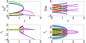
Figure 4: The four panels show the same diagnostics as in the previous figure but now for $\alpha=1$, $b=2$, and $k=1$.

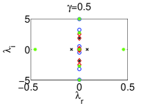
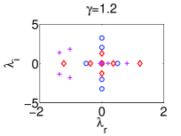
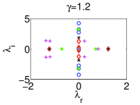
Figure 5: Stability plots. The top two panels are for $\alpha=0$, and the bottom one is when $\alpha=1$. In the case $\alpha=0$, at $\gamma=\gamma_{cr}^{(2)}=1$, one pair of blue circles and two pairs of red diamonds collide at 0 so that one pair of real eigenvalues arises in blue circles branch whereas two pairs of real eigenvalues arise in the red diamonds branch. The asymmetric branches only exist (and are unstable) for the smaller value of $\gamma=0.5$, for $\alpha=0$. For the same parameters ($b=2$, $k=1$), in the case of $\alpha=1$, the excited symmetric and both asymmetric branches are unstable for $\gamma=1.2$.

V Dynamics of the polarization

To examine the potentially symmetry breaking (and more generally instability driven) nature of the dynamical evolution past the critical points identified above, we have also performed direct numerical simulations which are illustrated in Fig. 6; see also Fig. 7. Here, it can be seen that although the relevant parameters are below the critical point for the linear ${\cal PT}$-phase transition $\gamma_{cr}^{(1)}=\sqrt{2}k$, nevertheless, symmetry breaking phenomena are observed due to the dynamical instability of the relevant states (the ones denoted by dashed lines in Fig. 2). This dynamics may, in principle, be associated with the so-called ghost states of complex propagation constant that have recently been proposed as relevant for the dynamical evolution in R46 . To substantiate this claim, we note that it is observed in the left panel of Fig. 6 that the relative phase of the two gain sites that lock into an equal growing amplitude, is $\pi/2$, as is those of the decaying amplitude lossy sites. In light of this, we seek ghost states with precisely this phase difference and are able to explicitly identify them via the ansatz $w_{3}=iw_{1},\ w_{4}=iw_{2}$, setting $w_{j}=c_{j}e^{i\phi_{j}}$ for $j=1,2$. For these branches, the propagation constant is complex. This highlights the potential growth or decay of such states. Importantly also, note that these states are “ghosts” because they may be solving the stationary problem of Eqs. (3), but the U$(1)$ invariance of the original model does not permit them to be a solution of the dynamical Eqs. (2).

The algebraic conditions that this family of solutions satisfies are

$$\sin\phi_{b}=\frac{(c_{2}^{2}-c_{1}^{2})\gamma}{(c_{1}^{2}+c_{2}^{2})B}$$ (28)

$$\cos\phi_{b}=\frac{(5-\alpha)(c_{1}^{2}+c_{2}^{2})}{3B}$$ (29)

$$\sin(\phi_{2}-\phi_{1})$$

$$= \frac{(3\gamma-B(\sin\phi_{b}+\cos\phi_{b})+(5-\alpha)c_{2}^{2})c_{2}}{6kc_{1}}$$ (30)

$$= \frac{(3\gamma+B(\sin\phi_{b}-\cos\phi_{b})+(5-\alpha)c_{1}^{2})c_{1}}{6kc_{2}}$$ (31)

$$\cos(\phi_{2}-\phi_{1})$$

$$= \frac{(3\gamma-B(\sin\phi_{b}-\cos\phi_{b})-(5-\alpha)c_{2}^{2})c_{2}}{6kc_{1}}$$ (32)

$$= \frac{(3\gamma+B(\sin\phi_{b}+\cos\phi_{b})-(5-\alpha)c_{1}^{2})c_{1}}{6kc_{2}}.$$ (33)

Notice that the imaginary part of the propagation constant $B\sin(\phi_{b})$ is proportional to the difference $c_{1}^{2}-c_{2}^{2}$. Hence, prior to the symmetry breaking, the relevant solutions bear a real propagation constant. Past the bifurcation point one (unstable) branch has $c_{2}^{2}>c_{1}^{2}$, while the stable branch has $c_{1}^{2}>c_{2}^{2}$. The relevant ghost state branches and their bifurcation from the equal amplitude ones are explored in Fig. 3-4. Given that these are only ghost solutions of the original dynamical problem, the interpretation of their linearization spectrum (shown for completeness in Fig. 5) is still an open problem.

These ghost states appear, in fact, to exhibit very similar evolution dynamics to regular unstable states. To illustrate this, we observed the particular behavior of the unstable modes and how it depends on the form of the initial perturbation. A typical example in which the gain sites lead to growth and the lossy sites to decay is shown in the left panel of Fig. 6. It is interesting that the evolution appears to be very proximal to that of the ghost states identified above. This is clearly showcased in Fig. 7, through the comparison of the growth pattern in the relevant sites (and the decay pattern in the lossy sites) with the exact, shifted in the propagation distance to fit the onset of growth, ghost state solution for the same parameters. On the other hand, in the right panel of Fig. 6 a different scenario of evolution is illustrated. Instead of the gain nodes growing and the lossy ones decaying, a breathing oscillation settles between the two pairs. These two scenarios, illustrated in Fig. 6, are the prototypical instability evolution ones that we have obtained in this system.

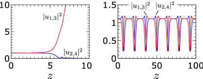
Figure 6: (Color online) Dynamics of an unstable circularly polarized mode at $b=3$, $\gamma=0.5$ and for $\alpha=0$ for two different small initial perturbations. The result of the evolution of the left panel involves growth at the gain sites ($u_{1,3}$, red curves in the color online version) and decay at the lossy sites ($u_{2,4}$, blue curves in the color online version). Notice that intensities among the two gain sites and among the two lossy sites are approximately equal ($|u_{1}|^{2}\approx|u_{3}|^{2}$ and $|u_{2}|^{2}\approx|u_{4}|^{2}$) and are not distinguishable in the scale of the plots. In the right panel only the initial stage of the found persistent periodic dynamics is shown; the simulations were performed up to $z=2000$.

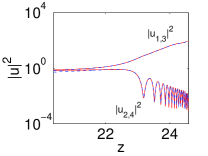
Figure 7: The dynamical semi-log plot of the ghost state with $\alpha=0$, $b=2$, and $k=1$ for $\gamma=1.02$. The red solid line and blue dashed line correspond to the red diamond and magenta plus branches in Fig. 3, respectively. The blue dashed line is plotted with a shift in time, i.e. delay by $z=19.61$. The time axis in the plot is the actual time of the red solid line. Their dynamical behaviors are essentially identical (and can not be distinguished on the scale of the plot), showcasing how the unstable dynamics of the red diamond branch is similar to that of the bifurcating ghost.

VI Conclusion

In conclusion, in the present work, we have proposed a novel, physically realistic variant of a ${\cal PT}$ symmetric dimer where the effect of birefringence has been taken into consideration. The existence of polarization of the electric field within the coupler yields two complex dynamical equations for each of the fibers, providing a physical realization of a plaquette model with both linear and nonlinear coupling between the elements. The stationary states of the model were identified and both linear and nonlinear ${\cal PT}$-phase transitions were obtained. The degenerate nature of the linear limit complicated the problem in comparison to other ones studied earlier in this context. Furthermore, the emergence of symmetry breaking phenomena and associated (subcritical or supercritical) pitchfork bifurcations, as well as their dynamical implications in leading to indefinite growth and decay (of the corresponding waveguide amplitudes) were elucidated. A connection was also given to ghost states.

From the physical point of view, we emphasize that the use of ${\cal PT}$ symmetry significantly changes the stability of the modes with different polarizations. For example, in the case of large propagation constant mismatches, we saw that the symmetric (circularly polarized) states become destabilized in the presence of gain/loss and may even cease to exist past a certain critical point of the relevant parameter. Instead of them, the dynamics may lead to a breathing exchange of “mass” between the gain and the lossy waveguides, or most commonly an indefinite growth of the former at the expense of the latter. This is in line with what is observed also in the evolution of the emerging ghost states of the system. The instabilities and associated dynamics should be observable in suitable generalizations of existing experiments such as kip . Such properties are relevant also to possibilities of solitonic (waveguide-array) generalizations of the coupler system as well as towards a possible use of ${\cal PT}$ symmetric coupler for measurement techniques based on the use of several nonlinear modes.

From the mathematical point of view, we believe that these studies may pave the way for considering multi-component, as well as multi-dimensional (generalizing the plaquettes considered here or those of guenther ) lattice models of ${\cal PT}$-symmetric form. In generalizing to multi-plaquette configurations, it would be especially interesting to examine which of the symmetry-breaking and nonlinear ${\cal PT}$-phase transition phenomena examined herein are preserved and what new phenomena may arise as additional degrees of freedom are added. Such studies will be deferred to future publications.

- (1) H. Ramezani, T. Kottos, R. El-Ganainy and D. N. Christodoulides, Phys. Rev. A 82, 043803 (2010).
- (2) M. C. Zheng, D. N. Christodoulides, R. Fleischmann and T. Kottos, Phys. Rev. A 82, 010103(R) (2010).
- (3) C. E. Rüter, K. G. Makris, R. El-Ganainy, D. N. Christodoulides, M. Segev, D. Kip, Nature Phys. 6, 192 (2010).
- (4) K. Li and P. G. Kevrekidis, Phys. Rev. E 83, 066608 (2011).
- (5) A. A. Sukhorukov, Z. Xu and Yu. S. Kivshar, Phys. Rev. A 82, 043818 (2010).
- (6) F. Kh. Abdullaev, V.V. Konotop, M. Ögren and M. P. Sørensen, Opt. Lett. 36, 4566 (2011).
- (7) R. Driben and B. A. Malomed, Opt. Lett. 36, 4323 (2011).
- (8) R. Driben and B. A. Malomed, Europhys. Lett. 96, 51001 (2011).
- (9) I. V. Barashenkov, S. V. Suchkov, A. A. Sukhorukov, S. V. Dmitriev, and Yu. S. Kivshar, Phys. Rev. A 86, 053809 (2012).
- (10) N. V. Alexeeva, I. V. Barashenkov, A. A. Sukhorukov, and Yu. S. Kivshar, Phys. Rev. A 85, 063837 (2012).
- (11) Yu. V. Bludov, V. V. Konotop, and B. A. Malomed, Phys. Rev. A 87, 013816 (2013).
- (12) H. Cartarius and G. Wunner, Phys. Rev. A 86, 013612 (2012); H. Cartarius, D. Haag, D. Dast and G. Wunner, J. Phys. A 45, 444008 (2012);
- (13) E.-M. Graefe, J. Phys. A 45, 444015 (2012).
- (14) A. S. Rodrigues, K. Li, V. Achilleos, P. G. Kevrekidis, D. J. Frantzeskakis, C. M. Bender, arXiv:1207.1066.
- (15) A. Regensburger, C. Bersch, M.-A. Miri, G. Onishchukov, D. N. Christodoulides and U. Peschel, Nature 488, 167 (2012).
- (16) C. R. Menyuk IEEE J. Quant. Eelectron., 23, 174-176 (1987)
- (17) D. A. Zezyulin and V. V. Konotop, Phys. Rev. Lett. 108 213906 (2012).
- (18) A. W. Snyder and Y. Chen, Opt. Lett. 14, 517 (1989); Y. Chen, A. W. Snyder, and D. N. Payne, IEEE J. Quant. Electro. 28, 239 (1992); M. Romagnoli S. Trillo, S. Wabnitz, Opt. and Quant. Electron. 24, S1237 (1992).
- (19) K. Li, P.G. Kevrekidis, B. A. Malomed and U. Guenther, J. Phys. A: Math. Theor. 45 444021 (2012).
- (20) V. Achilleos, P.G. Kevrekidis, D.J. Frantzeskakis, and R. Carretero-González Phys. Rev. A 86, 013808 (2012).