Right-angled billiards and volumes of moduli spaces of quadratic differentials on ${\mathbb{C}}\!\operatorname{P}^{1}$

Abstract.

We use the relation between the volumes of the strata of meromorphic quadratic differentials with at most simple poles on ${\mathbb{C}}\!\operatorname{P}^{1}$ and counting functions of the number of (bands of) simple closed geodesics in associated flat metrics with singularities to prove a very explicit formula for the volume of each such stratum conjectured by M. Kontsevich a decade ago.

Applying ergodic techniques to the Teichmüller geodesic flow we obtain quadratic asymptotics for the number of (bands of) closed trajectories and for the number of generalized diagonals in almost all right-angled billiards.

1. Introduction

Motivated by the study of computing asymptotics for the number of generalized diagonals and for the number of closed billiard trajectories in right-angled polygons, we were naturally led to questions on Masur–Veech volumes of strata of moduli spaces of quadratic differentials on ${\mathbb{C}}\!\operatorname{P}^{1}$. Our main result, explicitly computing these volumes, resolves a conjecture of M. Kontsevich.

1.1. Volumes of moduli spaces of quadratic differentials

Theorem 1.1 (Kontsevich Conjecture).

The volume of any stratum ${\mathcal{Q}}_{1}(d_{1},\dots,d_{k})$ of meromorphic quadratic differentials with at most simple poles on ${\mathbb{C}}\!\operatorname{P}^{1}$ (i.e. $d_{i}\in\{-1\,;\,0\}\cup\mathbb{N}$ for $i=1,\dots,k$, and $\sum_{i=1}^{k}d_{i}=-4$) is equal to

(1.1) $$\operatorname{Vol}{\mathcal{Q}}_{1}(d_{1},\dots,d_{k})=2\pi^{2}\cdot\prod_{i=1}^{k}v(d_{i})$$

(where all the zeroes and poles are “named”.)

Here, the function $v$ is defined on integers $n$ greater than or equal to $-1$ by

(1.2) $$v(n):=\cfrac{n!!}{(n+1)!!}\cdot\pi^{n}\cdot\begin{cases}\pi&\text{ when $n$ is odd}\\ 2&\text{ when $n$ is even}\end{cases}$$

for $n=-1,0,1,2,3\dots$, and the double factorial $n!!=n\cdot(n-2)\cdot\dots$ is the product of all even (respectively odd) positive integers smaller than or equal to $n$. By convention we set

$$(-1)!!=0!!=1\ ,$$

which implies that

$$v(-1)=1\qquad\text{and}\qquad v(0)=2.$$

This formula for the volume (up to some normalization factor) was conjectured by M. Kontsevich about ten years ago. It is much simpler than the formula for the volumes of the strata of Abelian differentials found by A. Eskin and A. Okounkov [EO01].

When this paper was written, there was not a single stratum of quadratic differentials for which the explicit volume was known, though an algorithm of computation was presented in [EO06]. In addition to this work, there is some very recent progress in evaluation of volumes of low-dimensional strata in genera different from $0$. Rigorous formal methods used in [Gj15] (in particular, implementation of the algorithm [EO06]) are confirmed by independent numerical experiments [DGZZ14]. However, any known approach involves significant computer-assisted computations, and is limited to volumes of strata of sufficiently small dimension, while Theorem 1.1 provides a simple formula for all strata in genus $0$.

Returning to our original motivation, we obtain as an important application of Theorem 1.1 asymptotics for the number of closed trajectories and for the number of generalized diagonals in right-angled polygons (see §1.3 below). This choice is particularly natural in the context of this paper since we have to solve an analogous problem for quadratic differentials and to compute the corresponding Siegel–Veech constants $c_{\mathcal{C}}$ for the strata of quadratic differentials in genus $0$ anyway: it makes part of the proof of Theorem 1.1. This theorem also immediately provides asymptotics for certain Hurwitz numbers, see §1.2. Another example of applications is discussed in [DZ15] where the values of volumes and the related Siegel–Veech constants are used to compute Lyapunov exponents of the Hodge bundle over hyperelliptic loci in the strata of quadratic differentials and to compute the diffusion rate for interesting families of generalized wind-tree billiards [DHL14].

Strategy of the proof.

We start by solving the counting problems for quadratic differentials. The Siegel–Veech constant $c_{\mathit{area}}$ responsible for the exact quadratic asymptotics of the weighted number of bands of regular closed geodesics on almost any flat sphere in a given stratum ${\mathcal{Q}}(d_{1},\dots,d_{n})$ of meromorphic quadratic differentials with at most simple poles on ${\mathbb{C}}\!\operatorname{P}^{1}$ was recently computed in [EKZ14],

(1.3) $$c_{\mathit{area}}({\mathcal{Q}}(d_{1},\dots,d_{n}))=-\cfrac{1}{8\pi^{2}}\,\sum_{j=1}^{n}\cfrac{d_{j}(d_{j}+4)}{d_{j}+2}\,.$$

Developing techniques elaborated in [EMZ03] for the strata of Abelian differentials and using the further results from [Bo09] and [MZ08] on the principal boundary of the strata of quadratic differentials we express the Siegel–Veech constant $c_{\mathit{area}}$ in genus $0$ in terms of the ratio of the volumes of appropriate strata,

(1.4) $$c_{\mathit{area}}({\mathcal{Q}}(d_{1},\dots,d_{n}))=\frac{\text{Explicit polynomial in volumes of simpler strata}}{\operatorname{Vol}({\mathcal{Q}}(d_{1},\dots,d_{n}))}\,.$$

In this way we obtain a series of identities on the volumes of the strata of meromorphic quadratic differentials with at most simple poles in genus zero. The resulting identities recursively determine the volumes of all strata. The proof of Theorem 1.1, given in §5, consists in verifying that the expression (1.1) for the volume satisfies the combinatorial identities implied by (1.3) and (1.4). Part of this verification is performed in Appendix A.

Remark 1.2 (Normalization conventions).

Note that the convention that all zeroes and poles are “named” affects the normalization: we compute the volumes of the corresponding covers over strata with “anonymous” singularities. For example, the stratum ${\mathcal{Q}}(1,-1^{5})$ of quadratic differentials with “anonymous” zeroes and poles is isomorphic to the stratum ${\mathcal{H}}(2)$ of holomorphic Abelian differentials; by convention the volume elements are chosen to be invariant under this isomorphism. However, by (1.1) we have

$$\operatorname{Vol}{\mathcal{Q}}_{1}(1,-1^{5})=2\pi^{2}\cdot v(1)\cdot\left(v(-1)\right)^{5}=2\pi^{2}\cdot\frac{\pi^{2}}{2}\cdot 1^{5}=5!\cdot\frac{\pi^{4}}{120}=5!\cdot\operatorname{Vol}{\mathcal{H}}_{1}(2)\,,$$

which corresponds to $5!$ ways to give names to five simple poles.

Similarly,

$$\operatorname{Vol}{\mathcal{Q}}_{1}(2,-1^{6})=2\pi^{2}\cdot v(2)\cdot\left(v(-1)\right)^{6}=2\pi^{2}\cdot\frac{4\pi^{2}}{3}\cdot 1^{6}=\frac{6!}{2!}\cdot\frac{\pi^{4}}{135}=\frac{6!}{2!}\cdot\operatorname{Vol}{\mathcal{H}}_{1}(1,1)\,.$$

This time there is an extra factor $\frac{1}{2!}$ responsible for forgetting the names of the two zeroes of ${\mathcal{H}}(1,1)$.

1.2. Counting pillowcase covers

One of the ways to compute the volumes of the strata of Abelian or quadratic differentials (actually, the only one before the current paper) is to count square-tiled surfaces or pillowcase covers, see [EO01], [EO06], [EOP], [Z00]. In the current paper we follow an alternative method, and, thus, our result implies an explicit expression for the leading term of the function counting associated pillowcase covers, when the degree of the cover tends to infinity.

Namely, following [EO06] we define a pillowcase cover of degree $4d$ as a ramified cover

(1.5) $$\pi:\hat{\mathcal{P}}\rightarrow\mathcal{P}$$

over the pillowcase orbifold $\mathcal{P}=\big{(}{\mathbb{C}}/(\mathbb{Z}\oplus i\mathbb{Z})\big{)}/\pm$ (as in Figure 1) with ramification data given as follows. Let $\eta$ be a partition and $\nu$ a partition of an even number into odd parts. Viewed as a map to the sphere, $\pi$ has profile $(\nu,2^{2d-|\nu|/2})$ over $0\in\mathcal{P}$ and profile $(2^{2d})$ over the other three corners of $\mathcal{P}$. Additionally, $\pi$ has profile $(\eta_{i},1^{4d-\eta_{i}})$ over $\ell(\eta)$ given points of $\mathcal{P}$ and unramified elsewhere, where $\ell(\eta)$ is the number of parts in $\eta$. This ramification data determines the genus $g$ of $\hat{\mathcal{P}}$ by

$$2-2g=\chi(\hat{\mathcal{P}})=\ell(\eta)+\ell(\nu)-|\eta|-|\nu|/2\,.$$

We consider only those ramification data for which $g=g(\hat{\mathcal{P}})$ in the above formula is equal to zero,

(1.6) $$\ell(\eta)+\ell(\nu)-|\eta|-|\nu|/2=2\,.$$

Figure 1. Pillowcase orbifold.

Denote by $\operatorname{Cov}^{0}_{4d}(\eta,\nu)$ the number of inequivalent degree $4d$ connected covers $\pi:\hat{\mathcal{P}}\to\mathcal{P}$ with ramification data $(\eta,\nu)$.

Denote by ${\mathcal{Q}}(\eta,\nu)$ the moduli space of quadratic differentials with singularity data $\{\nu_{i}-2\}$ and $\{2\eta_{i}-2\}$. Condition (1.6) guarantees that ${\mathcal{Q}}(\eta,\nu)$ is nonempty, and corresponds to genus zero.

Consider now the same partitions $\eta,\nu$ as above and a ramified cover

$$\pi_{\scriptscriptstyle\boxplus}:\hat{\mathcal{P}}\rightarrow\mathcal{P}$$

of the same degree $4d$ over the pillowcase orbifold $\mathcal{P}$ with ramification data given as follows: $\pi_{\scriptscriptstyle\boxplus}$ has profile $(2\eta,\nu,2^{2d-|\eta|-|\nu|/2})$ over $0\in\mathcal{P}$ and profile $(2^{2d})$ over the other three corners of $\mathcal{P}$. The cover $\pi_{\scriptscriptstyle\boxplus}$ is unramified elsewhere. Applying the Riemann–Hurwitz formula and using relation (1.6) we see that covers with such ramification profile again have genus zero. The corresponding flat surface belongs to the same stratum ${\mathcal{Q}}(\eta,\nu)$ as before. Denote by $\operatorname{Cov}^{0,{\scriptscriptstyle\boxplus}}_{4d}(\eta,\nu)$ the number of inequivalent degree $4d$ connected covers $\pi_{\scriptscriptstyle\boxplus}:\hat{\mathcal{P}}\to\mathcal{P}$ with ramification data $(\eta,\nu)$ as above.

Theorem 1.1 and the Theorem 1.3 below provide very simple asymptotic formulae for the Hurwitz numbers $\operatorname{Cov}^{0}_{4d}(\eta,\nu)$ and $\operatorname{Cov}^{0,{\scriptscriptstyle\boxplus}}_{4d}(\eta,\nu)$.

Theorem 1.3.

For any ramification data $(\eta,\nu)$ satisfying condition (1.6) the numbers $\operatorname{Cov}^{0}_{4d}(\eta,\nu)$ and

$\operatorname{Cov}^{0,{\scriptscriptstyle\boxplus}}_{4d}(\eta,\nu)$ of pillowcase covers of type $(\eta,\nu)$ admit the following limits:

(1.7) $$\lim_{N\to\infty}\frac{1}{N^{\ell(\eta)+\ell(\nu)-2}}\sum_{d=1}^{N}\operatorname{Cov}^{0}_{4d}(\eta,\nu) =2^{\ell(\eta)}\cdot\frac{\operatorname{Vol}{\mathcal{Q}}_{1}(\eta,\nu)}{2(\ell(\eta)+\ell(\nu)-2)}\,,$$

(1.8) $$\lim_{N\to\infty}\frac{1}{N^{\ell(\eta)+\ell(\nu)-2}}\sum_{d=1}^{N}\operatorname{Cov}^{0,{\scriptscriptstyle\boxplus}}_{4d}(\eta,\nu) =\frac{\operatorname{Vol}{\mathcal{Q}}_{1}(\eta,\nu)}{2(\ell(\eta)+\ell(\nu)-2)}\,,$$

where $\operatorname{Vol}{\mathcal{Q}}_{1}(\eta,\nu)$ is given by equation (1.1).

Theorem 1.3 is proved in §B.2.

Note that the more natural direct geometric approach to the counting of pillowcase covers leads to rather involved combinatorial problems. We present this alternative geometric approach in a separate paper [AEZ13].

Remark 1.4.

There are several different combinatorial approaches to computing volumes of strata, based on counting (pillowcase) covers.

For the strata of Abelian differentials, the problem is solved in [EO01]; see also [Z00] for a more direct but much less efficient approach. Many of these combinatorial approaches can be pushed to produce some complicated expressions for the volumes in Theorem 1.1. Currently, the most efficient approach to calculation of volumes of strata of quadratic differentials (independently of genus) is suggested in [EO06]. The exact values of volumes of all strata up to dimension $11$ are presented in [Gj15] based on the algorithm of [EO06]; this result is close to limits of current computational capacities of modern computers in manipulating huge tables of characters. For an approach based on Kontsevich’ solution to the Witten conjecture [K92] see [AEZ13]; one more version developing ideas of Eskin and Okounkov is suggested in [R-Z12]; see also [DGZZ14] for yet another approach. Paper [Gj15] suggests a comparison of various approaches.

However, we were not able to get the simple expressions (1.1) using any of these methods. In fact, our proof of Theorem 1.1 is not purely combinatorial, but has analytic, geometrical and dynamical inputs (and is motivated by consideration of Lyapunov exponents). It thus remains a challenge to give a more direct proof of Theorem 1.1, in particular bypassing [EKZ14].

1.3. Counting trajectories of right-angled billiards

Currently it is not known whether there exists a single closed billiard trajectory in every obtuse triangle (see [S08] for some progress in this direction and for further references). The situation with billiards in rational polygons (that is in polygons with angles which are rational multiples of $\pi$) is understood much better: trajectories of such billiards are related to geometry of certain compact flat surfaces with conical singularities, which are thoroughly studied starting with the landmark papers of H. Masur [M82] and W. Veech [Ve82]. In particular, it is known that a billiard in any rational polygon has infinitely many closed trajectories [KMS86], and furthermore the number of trajectories of length at most $L$ is bounded between $c_{1}L^{2}$ and $c_{2}L^{2}$ for some $0<c_{1}<c_{2}$ and for $L$ large enough, see [M88] and [M90].

In the current paper we study families of right-angled billiards like the ones in Figures 2 and 3. Namely, we assume that the billiard table is a topological disk endowed with a flat metric, and that the boundary of the disk is piecewise geodesic such that the angle at every corner of the boundary is an integer multiple of $\frac{\pi}{2}$. Note that by allowing integer multiples $k\pi/2$ with $k\geq 5$, we can obtain billiard tables which may not be embeddable in the plane (see Figure 2). In particular, we can consider helical right-angled billiards.

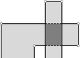
Figure 2. A Right-angled billiard table which is not embeddable into the plane.

We consider families of polygons sharing the same collection of interior corner angles $\left(\frac{\pi}{2}k_{1},\frac{\pi}{2}k_{2},\ldots,\frac{\pi}{2}k_{n}\right)$. Actually, it will be convenient to consider a slightly larger space ${\mathcal{B}}(k_{1},\ldots,k_{n})$ of “directional billiards” distinguishing a billiard table $\Pi$ and the same table turned by angle $\phi$. The measure in the space ${\mathcal{B}}(k_{1},\dots,k_{n})$ is the product measure of Lebesgue measure arising from the side lengths and the angular measure $d\phi$.

We count the number of generalized diagonals of bounded length in such billiards (that is, the number of trajectories of bounded length which start in some fixed corner $P_{i}$ and arrive to some fixed corner $P_{j}$, see Figure 3) and the number of closed billiard trajectories of bounded length. Note, that closed regular trajectories are never isolated in rational billiards: they always form bands of “parallel” closed trajectories of the same length, see Figure 3. Thus, when counting closed trajectories one actually counts the number of such bands. Sometimes, it is natural to count the bands with a weight which registers the thickness of the band, see e.g. Theorem 1.9 at the end of §1.3. By convention we always count non-oriented generalized diagonals and non-oriented closed billiard trajectories.

To give an idea of the general theorems stated in detail in §2 and developed in §4, we present the following representative results.

Theorem 1.5.

For any right-angled billiard $\Pi$ outside of a zero measure set in any family ${\mathcal{B}}(k_{1},\ldots,k_{n})$ the number $N_{ij}(\Pi,L)$ of generalized diagonals of length at most $L$ joining a pair of fixed corners $P_{i},P_{j}$ with angles $\frac{\pi}{2}$ has the following quadratic asymptotics as $L\to\infty$:

(1.9) $$N_{ij}(\Pi,L)\sim\cfrac{1}{2\pi}\cdot\cfrac{L^{2}}{\text{Area of the billiard table}}\ .$$

Theorem 1.5 is proved in  §4.11, using the theorem proved by Jon Chaika in Appendix C.

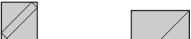
Figure 3. A family ${\mathcal{B}}(k_{1},\dots,k_{n})$ of right-angled polygons; a band of periodic trajectories on the left, and a generalized diagonal on the right.

The fact that this asymptotics does not depend at all on the billiard table is at the first glance counterintuitive. What is even more surprising is that it is universal: it is the same not only for almost all billiard tables inside each family, but it does not vary even from one family to another! In particular, though the shape of the two polygons of the same area in Figure 3 is quite different, the number of trajectories of length at most $L$ joining the right-angle corner $P_{i}$ to the right-angle corner $P_{j}$ is approximately the same in both cases, and is approximately the same as the number of trajectories of length at most $L$ joining two corners of the usual rectangular billiard of the same area when $L\gg 1$.

The situation becomes more complicated when we consider other types of corners of the billiard. Consider, for example, an $\operatorname{L}$-shaped billiard table as on Figure 4. Let $P_{1},\dots,P_{5}$ be the right-angle corners of the $\operatorname{L}$-shaped billiard, and let $P_{0}$ be the corner with the interior angle $\frac{3\pi}{2}$.

Figure 4. $\operatorname{L}$-shaped billiard.

Theorem 1.6.

For almost any $\operatorname{L}$-shaped billiard $\Pi$ the number $N_{i0}(\Pi,L)$ of generalized diagonals of length at most $L$ joining a fixed corner $P_{i}$ with angle $\frac{\pi}{2}$ and the corner $P_{0}$ with angle $\frac{3\pi}{2}$ has the following quadratic asymptotics as $L\to\infty$:

(1.10) $$N_{i0}(\Pi,L)\sim\cfrac{2}{\pi}\cdot\cfrac{L^{2}}{\text{Area of the billiard table}}\ .$$

The proof of this theorem also relies in part on Theorem C.1 proved by Jon Chaika in Appendix C.

The naive intuition does not help: the angle $\frac{3\pi}{2}$ at the corner $P_{0}$ is three times larger than in the previous case, while the constant in the asymptotics for the number of generalized diagonals is four times larger than in the previous statement. Currently we have no idea how to obtain this factor $4$ without using techniques of the Teichmüller geodesic flow, Lyapunov exponents of the Hodge bundle, and the computation of volumes of the moduli spaces of meromorphic quadratic differentials with at most simple poles on ${\mathbb{C}}\!\operatorname{P}^{1}$. Theorem 1.6 is proved in §4.9.

Using recently developed technology, one can prove weak asymptotic formulas similar to Theorem 1.5 and Theorem 1.6 for individual billiard tables. In particular, the following holds:

Theorem 1.7.

Suppose $\Pi$ is an $\operatorname{L}$-shaped billiard table as in Figure 4. Let

$$a=\frac{|P_{3}P_{4}|}{|P_{1}P_{2}|},\qquad b=\frac{|P_{2}P_{3}|}{|P_{4}P_{5}|}\,.$$

Then,

• If $a$ and $b$ are both rational, or if there exists a non-square integer $D>0$ such that $a,b\in\mathbb{Q}(\sqrt{D})$ and $a+\bar{b}=1$ (where $\bar{b}$ is the Galois conjugate of $b$), then

  (1.11) $$N_{ij}(\Pi,L)\sim c_{ij}\cfrac{L^{2}}{\text{Area of the billiard table}}\,,$$

• For any other $\operatorname{L}$-shaped billiard table, we have the “weak asymptotic formulas”

  $$N_{ij}(\Pi,L)\text{\ ``$\sim$''\ }\cfrac{1}{2\pi}\cdot\cfrac{L^{2}}{\text{Area of the billiard table}}\ .$$

  and

  $$N_{i0}(\Pi,L)\text{\ ``$\sim$''\ }\cfrac{2}{\pi}\cdot\cfrac{L^{2}}{\text{Area of the billiard table}}\ .$$

  The meaning of the “weak asymptotic  “$\sim$”  is defined in §2.2.

In the case (i) the Siegel–Veech constants $c_{ij}$ for rational values of parameters $a,b$ can be computed by the formula due to E. Gutkin and C. Judge [GJ00]. For $i,j\neq 0$ and $a,b\in\mathbb{Q}(\sqrt{D})$ the constants $c_{ij}$ are computed by M. Bainbridge, see [Ba07, Theorem 1.5 and §14].

Proof.

Theorem 1.7 is a compilation of several different results. In case (i), the polygon $\Pi$ is a Veech polygon, which gives rise to a Teichmüller curve, see [C04], [Mc03]. The existence of an asymptotic formula such as (1.11) for such a situation was proved in the pioneering work of W. Veech [Ve89].

Let

$$U=\begin{pmatrix}1&\ast\\ 0&1\end{pmatrix}\subset\operatorname{SL}(2,{{\mathbb{R}}}),\qquad P=\begin{pmatrix}\ast&\ast\\ 0&\ast\end{pmatrix}\subset\operatorname{SL}(2,{{\mathbb{R}}}).$$

The fact that weak asymptotic formulas such as those of part (ii) hold for any rational billiard table follows from [EMiMo, Theorem 2.12], which uses the general invariant measure classification theorem of [EMi] for the action of $P$ on moduli space. However, to evaluate the constant for an arbitrary $\operatorname{L}$-shaped table, one also has to appeal to the explicit classification of $\operatorname{SL}(2,{{\mathbb{R}}})$-invariant affine submanifolds in the moduli space of Abelian differentials in genus $2$ due to C. McMullen, [Mc07]. ∎

We note that asymptotic counting formulas for individual billiards are associated with invariant measure classification theorems on the action of subgroups of $\operatorname{SL}(2,{{\mathbb{R}}})$ on (certain subsets of) the moduli space. In particular, when a measure classification theorem for the action of the subgroup $U$ exists (e.g. in the case of a Teichmüller curve), one can get a strong asymptotic formula. Also, a measure classification theorem for the action of the subgroup $P$ leads to a weak asymptotic formula.

For other examples when a classification of invariant measures for the action of $U$ (and thus strong asymptotic formulas) are known see [EMS03], [EMM06], [CW10], [Ba10]. All examples of individual billiard tables for which the (strong) quadratic asymptotics was known are, essentially, covered by several families of triangles depending on one integer parameter; by several sporadic triangles beyond these families; by a square with a specially located barrier; and by a family of $\operatorname{L}$-shaped tables with or without a wall for special values of parameters of the $\operatorname{L}$-shaped table.

In §2.2 for each family ${\mathcal{B}}_{1}(k_{1},\ldots,k_{n})$ of right-angled billiards we describe all geometric types of generalized diagonals and all closed billiard trajectories which can be found on a billiard $\Pi$ outside of a zero measure set in ${\mathcal{B}}_{1}(k_{1},\ldots,k_{n})$. For such $\Pi$, and each such geometric type we prove (strong) quadratic asymptotics for the number of associated generalized diagonals (or of bands of closed billiard trajectories), and explicitly evaluate the constant in the quadratic asymptotics.

Theorem 1.8 below illustrates an application of the general Theorem 2.5 and of the general Theorems 4.3–4.8 to billiards more complicated than the $\operatorname{L}$-shaped ones, see Figure 5.

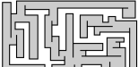
Figure 5. A billiard table from the family ${\mathcal{B}}(4^{m},3^{n},1^{m+n+4})$.

By ${\mathcal{B}}(4^{m},3^{n},1^{m+n+4})$ we denote the family of right-angled billiards with $m$ corners with angles $2\pi$ (endpoints of the walls); $n$ corners with interior angles $3\pi/2$, and with the remaining $n+m+4$ corners with interior angles $\pi/2$.

Theorem 1.8.

Consider two distinct corners $P_{i},P_{j}$ of a billiard $\Pi$ in any family ${\mathcal{B}}(4^{m},3^{n},1^{m+n+4})$. Assume that at least one of the interior angles $k_{i}\pi/2$ and $k_{j}\pi/2$ is different from $\pi/2$ (i.e. $k_{i},k_{2}$ are not simultaneously equal to $1$).

For almost any $\Pi$, any generalized diagonal $\delta$ joining $P_{i}$ to $P_{j}$ and non parallel to a side of $\Pi$ never bounds a band of closed trajectories. No other generalized diagonal in $\Pi$ has a segment parallel to any segment of $\delta$. For almost any $\Pi$, the number $N_{ij}(\Pi,L)$ of such generalized diagonals of length at most $L$ has the following asymptotics as $L\to+\infty$:

$$N_{ij}(\Pi,L)\sim c_{ij}\cdot\cfrac{L^{2}}{\text{Area of the billiard table}}\,,$$

where the constant $c_{ij}$ depends only on the angles $k_{i}\pi/2$ and $k_{j}\pi/2$ at $P_{i}$ and $P_{j}$ correspondingly; its value is presented in the following table:

$$\begin{array}[]{r|lll}\text{angle}&\cfrac{4\pi}{2}&\cfrac{3\pi}{2}&\cfrac{\pi}{2}\\[-6.0pt] \\ \hline\cr\cfrac{4\pi}{2}&\cfrac{9}{10}&\cfrac{45}{64}&\cfrac{9}{32}\\[-6.0pt] \\ \cfrac{3\pi}{2}&\cfrac{45}{64}&\cfrac{16}{3\pi^{2}}&\cfrac{2}{\pi^{2}}\\[-6.0pt] \\ \cfrac{\pi}{2}&\cfrac{9}{32}&\cfrac{2}{\pi^{2}}&\cfrac{1}{2\pi^{2}}\end{array}$$

Note that the values of the constants do not depend neither on the numbers $n$ or $m$ of corners, nor on the particular shape of the billiard. The proof of this theorem also relies in part on Theorem C.1 proved by Jon Chaika in Appendix C.

We complete this section with an illustration of further counting problems where one can apply our techniques. Let $N_{\mathit{area}}(\Pi,L)$ denote the number of bands of closed periodic billiard trajectories of length at most $L$ counted with a weight given by the normalized area of the band. More precisely, we count the area of overlapping domains of the band twice: the area of the band is naively measured as the area of the associated cylinder on the flat sphere, that is, the width of the band times the length of the closed trajectory, normalized by the area of the billiard table. Having measured the area of the band, we divide it by the area of the billiard table to get the weight of the band.

Theorem 1.9.

For any billiard $\Pi$ in any family ${\mathcal{B}}(k_{1},\dots,k_{n})$ of right-angled billiards the weighted number $N_{\mathit{area}}(\Pi,L)$ of bands of closed billiard trajectories of length at most $L$ satisfies the following weak asymptotics as $L\to\infty$:

$$N_{\mathit{area}}(\Pi,L)\text{\ ``$\sim$''\ }\cfrac{1}{16\pi}\,\sum_{j=1}^{n}\left(\cfrac{4}{k_{j}}-k_{j}\right)\cdot\cfrac{L^{2}}{\text{Area of the billiard table}}\ .$$

For almost any billiard $\Pi$ in the same family, the asymptotics is, actually, exact:

(1.12) $$N_{\mathit{area}}(\Pi,L)\sim\cfrac{1}{16\pi}\,\sum_{j=1}^{n}\left(\cfrac{4}{k_{j}}-k_{j}\right)\cdot\cfrac{L^{2}}{\text{Area of the billiard table}}\ .$$

The weak asymptotics for all billiards follows, as before, from [EMiMo, Theorem 2.12]. The strong asymptotics (1.12) is proved in  §6.1, using Jon Chaika’s Theorem C.1 which is proved in Appendix C. The constant in the corresponding counting function is directly related to the Siegel–Veech area constant for the corresponding stratum of meromorphic quadratic differentials on ${\mathbb{C}}\!\operatorname{P}^{1}$ discussed in §1.1.

1.4. Right-Angled billiard tables and quadratic differentials

Given a right-angled billiard $\Pi$ in ${\mathcal{B}}(k_{1},\dots,k_{n})$ we can glue a topological sphere from two superposed copies of $\Pi$ identifying the boundaries of the two copies by isometries, see Figure 6. By construction the resulting topological sphere is endowed with a flat metric. Note that the metric is regular on interior of the segments coming from the boundary of $\Pi$: one can unfold a neighborhood of any such point into a small regular flat domain.

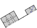
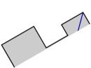
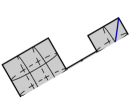
Figure 6. Flat spheres glued from two copies of a right-angled billiard. The angle by which the billiard table is rotated with respect to the horizontal position encodes the “phase” of the corresponding quadratic differential. A general generalized diagonal in the polygon gives rise to two distinct saddle connections on the flat sphere.

However, the resulting flat metric has conical singularities with cone angles $\pi k_{1},\dots,\pi k_{n}$ at the points coming from the vertices of $\Pi$. By construction the linear holonomy of the flat metric with isolated singularities belongs to the group $\mathbb{Z}/2\mathbb{Z}$: the parallel transport along a short path encircling a conical point $P_{j}$ brings a tangent vector $\vec{v}$ either to itself or to $-\vec{v}$ depending on the parity of $k_{j}$.

It is known that a flat metric with isolated conical singularities and with holonomy in $\mathbb{Z}/2\mathbb{Z}$ on a closed surface defines a complex structure and a meromorphic quadratic differential $q$ in this complex structure defined up to multiplication by a scalar $e^{i\phi}$. Choosing a line direction $\pm\vec{v}$ at some point of the resulting flat sphere as a “horizontal” direction we fix the scalar $e^{i\phi}$. In an appropriate flat local coordinate $z$ outside of the conical points the resulting quadratic differential has the form $(dz)^{2}$. A conical singularity with a cone angle $k_{i}\pi$ corresponds to a zero of the quadratic differential of degree $k_{i}-2$, where a “zero of degree $-1$” is a simple pole.

Actually, the two structures are synonymous: a meromorphic quadratic differential $q$ with at most simple poles on a Riemann surface defines a canonical flat metric with isolated conical singularities, with linear monodromy in $\mathbb{Z}/2\mathbb{Z}$ and with a distinguished foliation by straight lines in the flat metric (see the original papers [M82] and [Ve82] or surveys [MT99] and [Z03]).

By construction closed billiard trajectories in $\Pi$ are in canonical one-to-two correspondence with closed regular geodesics on the associated flat sphere, and generalized diagonals on $\Pi$ are in the natural one-to-two correspondence with the saddle connections on the associated flat sphere, see Figure 6. Thus, the two counting problems are closely related.

It is known by work of Veech [Ve98] and of Eskin-Masur [EM00] that almost all flat spheres in a given stratum ${\mathcal{Q}}(d_{1},\dots,d_{n})$ satisfy a quadratic asymptotic formula for the number of saddle connections. However, we cannot immediately translate this result to right-angled billiards. An elementary count shows that the space ${\mathcal{B}}(k_{1},\dots,k_{n})$ has real dimension $n-2$, while the associated stratum ${\mathcal{Q}}(k_{1}-2,\dots,k_{n}-2)$ has complex dimension $n-2$. Thus, flat spheres constructed from right-angled billiards form a subset of measure zero, and “almost all” results for the strata are not applicable to families of billiards. This is the common difficulty of translating results valid for flat surfaces to billiards.

In our specific case we are lucky enough to get a subspace of flat spheres “of billiard origin” which is transversal to the unstable foliation of the Teichmüller flow (see §3). This allows us to apply certain techniques of hyperbolic dynamics to obtain some ergodic results in slightly weaker form. As a corollary we obtain the desired information on quadratic asymptotics in the counting problems for almost all billiards. The corresponding ergodic technique is presented in §6. A key tool we use is Theorem C.1 proved by Jon Chaika in Appendix C.

1.5. Reader’s guide

The paper (like Caesar’s Gaul) is composed of three parts. The reader interested only in the billiards may read only §2 (and optionally §3 and §6). The ergodic theorem we use in §6 is due to Jon Chaika, and is proved in Appendix C.

The part where we compute the volume of any stratum ${\mathcal{Q}}_{1}(d_{1},\dots,d_{n})$ of meromorphic quadratic differentials with at most simple poles on ${\mathbb{C}}\!\operatorname{P}^{1}$ and where we compute the Siegel–Veech constants for these strata is independent from the rest of the paper. It is presented in §2.1, §§3.1–3.2 and in §§4–5 (with one verification in Appendix A).

Finally, Appendix B devoted to pillowcase covers is completely independent of the rest of the paper.

1.6. Historical remarks

The formula for the volume of the strata of quadratic differentials was guessed by M. Kontsevich more than a decade ago. At this time formula (1.3) related to Lyapunov exponents was known experimentally. The Siegel–Veech constant (1.4) has especially simple form for the strata ${\mathcal{Q}}(d,-1^{d+4})$ of quadratic differentials with a single zero and only simple poles on ${\mathbb{C}}\!\operatorname{P}^{1}$. Comparing (1.3) and a version of (1.4) M. Kontsevich obtained a conjectural formula for $\operatorname{Vol}{\mathcal{Q}}_{1}(d,-1^{d+4})$. Motivated by the simplicity of the resulting expression as a function of $d$ he stated a guess that $\operatorname{Vol}{\mathcal{Q}}_{1}(d_{1},\dots,d_{k})$ for any stratum in genus $0$ might be expressed as a product of the corresponding expressions for all $d_{i}$.

Acknowledgments

The authors are grateful to M. Kontsevich for the conjecture on the volumes and for collaboration in the work on Lyapunov exponents essential for the current paper.

Part of this paper strongly relies on techniques developed in collaboration with H. Masur. We are grateful to him for his very important contribution.

We thank C. Boissy for the list of configurations of ĥomologous saddle connections in genus $0$, elaborated specifically for our needs, and for his pictures of configurations.

We thank P. Paule for the kind permission to use the “MultiSum” package, which was helpful in developing certain intuition with the combinatorial identity.

We thank E. Goujard who carefully read the first version of this paper, provided us with a list of typos, and indicated to us a missing factor in formula (1.7) and necessity to prove Lemma B.3 as explained in Remark B.4.

We are grateful to P. Hubert and to anonymous referee whose suggestions helped to improve the presentation and clarity of the arguments.

The authors are happy to thank IHES, IMJ, IUF, MPIM, MSRI, and the Universities of Chicago, of Illinois at Urbana-Champaign, of Rennes 1, and of Paris 7 for hospitality during the preparation of this paper.

2. Configurations and Counting Theorems

2.1. Types of saddle connections and generalized diagonals

We distinguish the following four ways of getting generalized diagonals in a right-angled billiard. They correspond to four types of configurations of saddle connections on a flat sphere defined by a meromorphic quadratic differential with simple poles, see [EMZ03] and [MZ08] for general information on configurations of saddle connections and [Bo09] for specific case of ${\mathbb{C}}\!\operatorname{P}^{1}$.

I. Saddle connection joining distinct singularities. In this situation (see Figure 7) we have a generalized diagonal joining a corner $P_{i}$ with the inner angle $k_{i}\frac{\pi}{2}$, where $k_{i}\geq 3$, to a distinct corner $P_{j}$.

Figure 7. Type I. On the left: a generalized diagonal joining two distinct corners of the billiard, where at least one of the two corners has inner angle at least $\frac{3\pi}{2}$. It does not bound a band of closed trajectories. On the right: a saddle connection on ${\mathbb{C}}\!\operatorname{P}^{1}$ joining a zero to a distinct zero (or to a pole).

The induced flat metric on ${\mathbb{C}}\!\operatorname{P}^{1}$ has an associated saddle connection of the same length joining the zero $P_{i}$ to the distinct zero (or simple pole) $P_{j}$.

II. Saddle connection joining a zero to itself. This situation (see Figure 8) can happen only when we have a corner $P_{i}$ with a corner angle $k_{i}\frac{\pi}{2}$ with $k_{i}\geq 4$. In this case we can have a generalized diagonal joining the corner $P_{i}$ to itself such that it does not bound a band of closed regular trajectories.

Figure 8. Type II. On the left: a generalized diagonal returning to the same corner. For this type, it does not bound closed trajectories. On the right: the corresponding saddle connection joining a zero (of order at least $2$) to itself.

For the induced flat metric on ${\mathbb{C}}\!\operatorname{P}^{1}$ we get a corresponding saddle connection of the same length joining the zero $P_{i}$ to itself such that the total angle $k_{i}\pi$ at the singularity $P_{i}$ is split by the separatrix loop into two sectors having the angles strictly greater than $\pi$ (which is equivalent to the condition that generically such a saddle connection does not bound a cylinder filled with periodic geodesics).

III. A “pocket”. In this situation (see Figure 9) we have a band of periodic trajectories. The boundary of the band is composed of two generalized diagonals. The first generalized diagonal joins a pair of corners $P_{i}$, $P_{j}$ with inner angles $\frac{\pi}{2}$. The length of this saddle connection is twice shorter than the length of periodic billiard trajectory in the band. The second generalized diagonal joins a corner $P_{i}$ with inner angle $k_{i}\frac{\pi}{2}$ with $k_{i}\geq 3$ to itself. The length of this saddle connection is the same as the length of periodic billiard trajectory in the band.

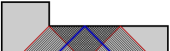
Figure 9. Type III. On the left: a band of closed trajectories bounded by two generalized diagonals. One of generalized diagonals joins two distinct corners with angles $\frac{\pi}{2}$; the other returns to the same corner. On the right: the corresponding “pocket” configuration with a cylinder bounded on one side by a saddle connection joining two simple poles, and by a saddle connection joining a zero to itself on the other side.

For the associated flat metric on ${\mathbb{C}}\!\operatorname{P}^{1}$ we get a cylinder filled with closed regular trajectories. One of the boundary components of the cylinder degenerates to a saddle connection joining two simple poles $P_{i}$, $P_{j}$. Clearly, this saddle connection is twice shorter than the length of the periodic trajectories. The other boundary component is a saddle connection joining the zero $P_{l}$ to itself. The total angle $k_{l}\pi$ at the singularity $P_{l}$ is split by the separatrix loop into two sectors, such that the sector adjacent to the cylinder has angle $\pi$. The length of this saddle connection is the same as the length of the periodic trajectories in the cylinder.

IV. A “dumbbell”. In this last situation (see Figure 10) we again have a band of periodic trajectories. The boundary of the band is again composed of two generalized diagonals, but this time the first generalized diagonal joins the corner $P_{i}$ with inner angle $k_{i}\frac{\pi}{2}$ to itself, and the second generalized diagonal joins the distinct corner $P_{j}$ with inner angle $k_{j}\frac{\pi}{2}$ to itself. Both $k_{i},k_{j}$ are greater than or equal to $3$. The length of each of these two generalized diagonals is the same as the length of every periodic billiard trajectory in the band.

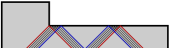
Figure 10. Type IV. On the left: a band of periodic trajectories, such that each of the two bounding generalized diagonals returns to the same corner. On the right: a “dumbbell” composed of two flat spheres joined by a cylinder. Each boundary component of the cylinder is a saddle connection joining a zero to itself.

For the associated flat metric on ${\mathbb{C}}\!\operatorname{P}^{1}$ we get a cylinder filled with closed regular trajectories. On each of the boundary components of the cylinder we have a saddle connection joining the zero $P_{i}$ (correspondingly $P_{j}$) to itself. The length of each of the two saddle connections is the same as the length of the periodic trajectories in the cylinder.

The following two Propositions explain why we distinguish these four particular types of configurations (see more details in  §3.2 which discusses a homological interpretation of these statements).

Proposition 2.1.

Almost any flat surface $S$ in any stratum ${\mathcal{Q}}_{1}(d_{1},\dots,d_{n})$ different from the pillowcase stratum ${\mathcal{Q}}_{1}(-1^{4})$ does not have a single pair of parallel saddle connections different from the pairs involved in configurations of types $I,II,III,IV$.

Proposition 2.1 is proved in  §3.2. An analogous statement can be formulated for right-angled billiards.

Proposition 2.2.

For almost any right-angled billiard in any family ${\mathcal{B}}(k_{1},\dots,k_{n})$ the following property holds. Consider a pair of trajectories, where each trajectory is either a closed regular trajectory or a generalized diagonal. Suppose that these trajectories are not parallel to any side of the polygon. If some segment of the first trajectory is parallel to some segment of the second trajectory, then both trajectories make part of one of configurations I–IV described in 2.1.

Proposition 2.2 mimics Proposition 7.4 in [EMZ03]; it is proved in  §3.3.

Configurations of saddle connections. In addition to the type I–IV of a saddle connection, we may specify some extra combinatorial information, for example the indices (“names”) of all singularities involved. For saddle connections of type IV, where a cylinder is joining two spheres, we specify not only the zeroes $P_{i}$ and $P_{j}$ at the boundary components of the cylinder, but we also specify the subcollections $P_{i_{1}},\dots,P_{i_{k_{1}}}$ and $P_{j_{1}},\dots,P_{j_{k_{2}}}$ of numbered zeroes an poles which get to the first and to the second sphere correspondingly. We call this information the configuration of a saddle connection (or the configuration of saddle connections, when there are several saddle connections involved as in types III and IV). By convention, the configuration of saddle connections includes its type. See also  §3.2 for a homological interpretation of a configuration of saddle connections.

Configuration of a generalized diagonal. By the configuration of the generalized diagonal we mean the configuration of the associated saddle connections in ${\mathbb{C}}\!\operatorname{P}^{1}$ described in §1.4.

2.2. Counting Theorems

By the notation

$$N(L)\sim cL^{2}$$

we mean as customary,

$$\lim_{L\to\infty}\frac{N(L)}{L^{2}}=c.$$

For technical reasons, we will need to consider “weak asymptotic formulas”

$$N(L)\text{\ ``$\sim$''\ }cL^{2}$$

which means

$$\lim_{L\to\infty}\frac{1}{L}\int_{0}^{L}N(e^{t})e^{-2t}\,dt=c.$$

The following theorem (which is a special case of results of [Ve98] and [EM00]) establishes a strong asymptotic formula for almost all flat surfaces in a stratum. By convention we always count non-oriented saddle connections and non-oriented closed flat geodesics.

Theorem 2.3.

For almost any flat surface $S$ in any stratum ${\mathcal{Q}}(d_{1},\dots,d_{n})$ of meromorphic quadratic differentials with at most simple poles on ${\mathbb{C}}\!\operatorname{P}^{1}$ the number $N_{\mathcal{C}}(S,L)$ of occurrences of saddle connections of length at most $L$ and of fixed configuration ${\mathcal{C}}$, has quadratic asymptotics in $L$:

$$N_{\mathcal{C}}(S,L)\sim c_{\mathcal{C}}\cdot\frac{\pi L^{2}}{\text{Area of }S}\,.$$

The constants $c_{\mathcal{C}}$ are called Siegel-Veech constants. They depend only on the configuration ${\mathcal{C}}$ and on $d_{1},\dots,d_{n}$. Their values are given in §4.

Theorem 2.3 is proved in §4.5. Note that Theorem 2.3 has no relation to billiards, it concerns only flat metrics on ${\mathbb{C}}\!\operatorname{P}^{1}$ induced by meromorphic quadratic differentials with simple poles. In §1.4 we described how a right-angled billiard table $\Pi$ canonically determines a meromorphic quadratic differential on ${\mathbb{C}}\!\operatorname{P}^{1}$. However, since the image of the resulting map ${\mathcal{B}}(k_{1},\dots,k_{n})\to{\mathcal{Q}}(k_{1}-2,\dots k_{n}-2)$ has measure $0$ in ${\mathcal{Q}}(k_{1}-2,\dots,k_{n}-2)$, results such as Theorem 2.3 do not immediately imply anything about right-angled billiards. Nevertheless, we have the following:

Theorem 2.4.

For almost any billiard table $\Pi$ in any family ${\mathcal{B}}(k_{1},\dots,k_{n})$ of right-angled billiards the number $N_{\mathcal{C}}(\Pi,L)$ of occurrences of generalized diagonals of configuration ${\mathcal{C}}$ and of length at most $L$ has quadratic asymptotics in $L$:

(2.1) $$N_{\mathcal{C}}(\Pi,L)\sim\frac{c_{\mathcal{C}}}{4}\cdot\frac{\pi L^{2}}{\text{Area of the billiard table }\Pi}\,,$$

where the constants $c_{\mathcal{C}}$ are the corresponding Siegel–Veech constants $c_{\mathcal{C}}$ for the stratum ${\mathcal{Q}}(k_{1}-2,\dots,k_{n}-2)$ in Theorem 2.3.

Theorem 2.4 is proved in §6.1, using Jon Chaika’s Theorem C.1 which is proved in Appendix C.

The factor of $\tfrac{1}{4}$ in (2.1) is explained as follows. Note that any generalized diagonal in the billiard table $\Pi$ which is not parallel to one of the sides of $\Pi$ canonically determines two symmetric saddle connections of the same type on the flat surface $S$ glued from the two copies of $\Pi$, where the symmetry is the antiholomorphic involution, see Figure 6. Hence,

$$N_{\mathcal{C}}(\Pi,L)=\frac{1}{2}N_{\mathcal{C}}(S,L)\,.$$

Note also, that by construction the area of $S$ is twice the area of the billiard table $\Pi$.

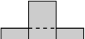
Figure 11. A helical billiard corresponds to the stratum ${\mathcal{Q}}(d,-1^{d+4})$.

Note that our billiard table does not need to be necessarily embeddable into the plane, say, we can consider a helical right-angled billiard as in Figure 11. More precisely, by a right-angled billiard table we call a topological disc endowed with a flat metric having the following properties. The flat metric is allowed to have isolated cone-type singularities in the interior of the disc with cone angles of the form $l_{i}\pi$, with $l_{i}\in\mathbb{N}$. The boundary of the disc is piecewise-geodesic in the flat metric, and the angles between the geodesic segments have the form $k_{j}\pi/2$, with $k_{j}\in\mathbb{N}$.

In fact, some version of Theorem 2.4 holds for individual billiards:

Theorem 2.5.

Suppose $\Pi$ is a billiard table from the family of right-angled billiards ${\mathcal{B}}(k_{1},\dots,k_{n})$. Furthermore, suppose $\Pi$ is such that the flat surface $S$ glued from two copies of $\Pi$ does not belong to any proper $\operatorname{GL}(2,{{\mathbb{R}}})$-invariant affine submanifold of the stratum ${\mathcal{Q}}(d_{1},\dots,d_{k})$. Then, for any choice I–IV of configuration ${\mathcal{C}}$, the weak asymptotic formula

$$N_{\mathcal{C}}(\Pi,L)\text{\ ``$\sim$''\ }\frac{c_{\mathcal{C}}}{4}\cdot\frac{\pi L^{2}}{\text{Area of the billiard table }\Pi}$$

holds, where $c_{\mathcal{C}}$ is the Siegel–Veech constant corresponding to the configuration ${\mathcal{C}}$ in the stratum ${\mathcal{Q}}(k_{1}-2,\dots,k_{n}-2)$ (as in Theorem 2.3).

Proof.

The statement is an immediate corollary of [EMiMo, Theorem 2.12]. ∎

We note that a complete proof of  [EMiMo, Theorem 2.12] involves the measure classification theorem of [EMi] and is well over 200 pages long, and yields weak asymptotic formulas. The proof of Theorem 2.4 is much shorter, and uses special features of right-angled billiards, namely Proposition 3.2. However, Theorem 2.4 is an almost everywhere statement, and does not imply any type of asymptotic formula for an individual billiard table.

We also note that for most other families of billiards, almost-everywhere statements like Theorem 2.4 are not available (since the analogue of Proposition 3.2 fails.)

3. Billiards in right-angled polygons and quadratic differentials

In  §3.1 we describe the cohomological coordinates in a stratum of quadratic differentials. We proceed in  §3.2 with a reminder of the notions of ĥomologous saddle connections and a configuration of ĥomologous saddle connections.

In  §3.3 we analyze the canonical embedding of the space of (directional) right-angled billiards ${\mathcal{B}}(k_{1},\dots,k_{n})$ into the corresponding space ${\mathcal{Q}}(k_{1}-2,\dots,k_{n}-2)$ of meromorphic quadratic differentials on ${\mathbb{C}}\!\operatorname{P}^{1}$. Namely, we prove in Proposition 3.2 that its image projects surjectively onto the unstable foliation of the Teichmüller geodesic flow, which allows us to apply certain ergodic techniques of hyperbolic dynamics not only to flat surfaces from ${\mathcal{Q}}(k_{1}-2,\dots,k_{n}-2)$ but to billiards from ${\mathcal{B}}(k_{1},\dots,k_{n})$.

We complete  §3 with a proof of Proposition 2.2.

3.1. Coordinates in a stratum of quadratic differentials.

Consider a meromorphic quadratic differential $\psi$ having zeroes of arbitrary multiplicities but only simple poles on ${\mathbb{C}}\!\operatorname{P}^{1}$. Let $P_{1},\ldots,P_{n}$ be its singular points (zeros and simple poles). Consider the minimal branched double covering $p:\hat{S}\to{\mathbb{C}}\!\operatorname{P}^{1}$ such that the induced quadratic differential $p^{\ast}\psi$ on the hyperelliptic surface $\hat{S}$ is a square of an Abelian differential $p^{\ast}\psi=\omega^{2}$.

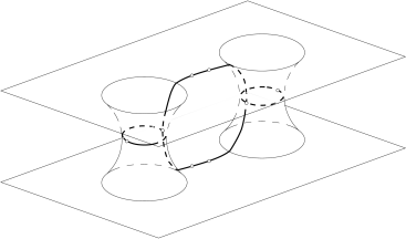
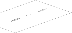
Figure 12. Basis of cycles in $H_{1}^{-}(\hat{S},\{\hat{P}_{1},\dots,\hat{P}_{N}\};\mathbb{Z})$. Note that the cycle corresponding to the very last slit is omitted.

The zeros $\hat{P}_{1},\ldots,\hat{P}_{N}$ of the resulting Abelian differential $\omega$ correspond to the zeros of $\psi$ in the following way: every zero $P\in{\mathbb{C}}\!\operatorname{P}^{1}$ of $\psi$ of odd order is a ramification point of the covering, so it produces a single zero $\hat{P}\in\hat{S}$ of $\omega$; every zero $P\in{\mathbb{C}}\!\operatorname{P}^{1}$ of $\psi$ of even order is a regular point of the covering, so it produces two zeros $\hat{P}^{+},\hat{P}^{-}\in\hat{S}$ of $\omega$. Every simple pole of $\psi$ defines a branching point of the covering; this point is a regular point of $\omega$.

Consider the subspace $H_{1}^{-}(\hat{S},\{\hat{P}_{1},\dots,\hat{P}_{N}\};\mathbb{Z})$ of the relative homology of the cover with respect to the collection of zeroes $\{\hat{P}_{1},\dots,\hat{P}_{N}\}$ of $\omega$ which is antiinvariant with respect to the induced action of the hyperelliptic involution. We are going to construct a basis in this subspace (in complete analogy with a usual basis of absolute cycles for a hyperelliptic surface).

We can always enumerate the singular points $P_{1},\dots,P_{n}$ of $\psi$ in such a way that $P_{n}$ is a simple pole. Chose now a simple oriented broken line $P_{1},\ldots,P_{n-1}$ on ${\mathbb{C}}\!\operatorname{P}^{1}$ joining consecutively all the singular points of $\psi$ except the last one. For every arc $[P_{i},P_{i+1}]$ of this broken line, $i=1,\dots,n-2$, the difference of their two preimages defines a relative cycle in $H_{1}^{-}(\hat{S},\{\hat{P}_{1},\dots,\hat{P}_{N}\};\mathbb{Z})$. By construction such a cycle is antiinvariant with respect to the hyperelliptic involution. It is immediate to see that the resulting collection of cycles forms a basis in $H_{1}^{-}(\hat{S},\{\hat{P}_{1},\dots,\hat{P}_{N}\};\mathbb{Z})$.

Note that a preimage of a simple pole does not belong to the set $\hat{P}_{1},\ldots,\hat{P}_{N}$. Thus, a preimage of an arc $[P_{i},P_{i+1}]$ having a simple pole as one of the endpoints does not define a cycle in $H_{1}(\hat{S},\{\hat{P}_{1},\dots,\hat{P}_{N}\};\mathbb{Z})$. However, since a simple pole is always a branching point, the difference of the preimages of such arc is already a well-defined relative cycle in $H_{1}(\hat{S},\{\hat{P}_{1},\dots,\hat{P}_{N}\};\mathbb{Z})$.

Let ${\mathcal{Q}}(d_{1},\dots,d_{n})$ be the ambient stratum for the meromorphic quadratic differential $({\mathbb{C}}\!\operatorname{P}^{1},\psi)$. The subspace $H^{1}_{-}(\hat{S},\{\hat{P}_{1},\dots,\hat{P}_{N}\};{\mathbb{C}})$ in the relative cohomology antiinvariant with respect to the natural involution defines local coordinates in the stratum.

3.2. Ĥomologous saddle connections

We follow the exposition in [MZ08] introducing the notions of a rigid collection of saddle connections and of ĥomologous saddle connections. Consider a flat sphere $S$ corresponding to a meromorphic quadratic differential $({\mathbb{C}}\!\operatorname{P}^{1},\psi)$ with at most simple poles. Any saddle connection on the flat sphere $S$ persists under small deformations of $S$ inside ${\mathcal{Q}}(\alpha)$. It might happen that any deformation of a given flat surface which shortens some specific saddle connection necessarily shortens some other saddle connections. We say that a collection $\{\gamma_{1},\dots,\gamma_{n}\}$ of saddle connections is rigid if any sufficiently small deformation of the flat surface inside the stratum preserves the proportions $|\gamma_{1}|:|\gamma_{2}|:\dots:|\gamma_{n}|$ of the lengths of all saddle connections in the collection.

Consider the canonical double cover $\hat{S}$ over $S$ defined in  §3.1. Given a saddle connection $\gamma$ on $S$ choose an orientation of $\gamma$ and let $\gamma^{\prime},\gamma^{\prime\prime}$ be its lifts to the double cover $\hat{S}$ endowed with the orientation inherited from $\gamma$. If $[\gamma^{\prime}]=-[\gamma^{\prime\prime}]$ as cycles in $H_{1}(\hat{S},\{\hat{P}_{1},\dots,\hat{P}_{N}\};\,\mathbb{Z})$ we let $[\hat{\gamma}]:=[\gamma^{\prime}]$, otherwise we define $[\hat{\gamma}]$ as $[\hat{\gamma}]:=[\gamma^{\prime}]-[\gamma^{\prime\prime}]$. It immediately follows from the above definition that the cycle $[\hat{\gamma}]$ defined by a saddle connection $\gamma$ is always primitive in $H_{1}(\hat{S},\{\hat{P}_{1},\dots,\hat{P}_{N}\};\,\mathbb{Z})$ and belongs to $H_{1}^{-}(\hat{S},\{\hat{P}_{1},\dots,\hat{P}_{N}\};\,\mathbb{Z})$.

Following [MZ08] we introduce the following

Definition 3.1.

The saddle connections $\gamma_{1},\gamma_{2}$ on a flat surface $S$ defined by a quadratic differential $q$ are ĥomologous if $[\hat{\gamma}_{1}]=[\hat{\gamma}_{2}]$ in $H_{1}(\hat{S},\hat{P};\,\mathbb{Z})$ under an appropriate choice of orientations of $\gamma_{1},\gamma_{2}$. (The notion “homologous in the relative homology with local coefficients defined by the canonical double cover induced by a quadratic differential” is unbearably bulky, so we introduced an abbreviation “ĥomologous”. We stress that the circumflex over the “h” is quite meaningful: as it is indicated in the definition, the corresponding cycles are homologous on the double cover.)

Note that since there is no canonical way to enumerate the preimages $\gamma^{\prime},\gamma^{\prime\prime}$ of a saddle connection $\gamma$ on the double cover, the cycle $[\hat{\gamma}]$ is defined only up to a sign, even when we fix the orientation of $\gamma$. Thus, $\gamma_{1}$ is ĥomologous to $\gamma_{2}$ if and only if $[\hat{\gamma}_{1}]=\pm[\hat{\gamma}_{2}]$.

Proposition (H. Masur, A. Z.).

Let $S$ be a flat surface corresponding to a meromorphic quadratic differential $q$ with at most simple poles. A collection $\gamma_{1},\dots,\gamma_{n}$ of saddle connections on $S$ is rigid if and only if all saddle connections $\gamma_{1},\dots,\gamma_{n}$ are ĥomologous.

There is an obvious geometric test for deciding when saddle connections $\gamma_{1},\gamma_{2}$ on a translation surface $S$ are homologous: it is sufficient to check whether $S\setminus(\gamma_{1}\cup\gamma_{2})$ is connected or not (provided $S\setminus\gamma_{1}$ and $S\setminus\gamma_{2}$ are connected). It is slightly less obvious to check whether saddle connections $\gamma_{1},\gamma_{2}$ on a flat surface $S$ with nontrivial linear holonomy are ĥomologous or not. In particular, a pair of closed saddle connections might be homologous in the usual sense, but not ĥomologous; a pair of closed saddle connections might be ĥomologous even if one of them represents a loop homologous to zero, and the other does not; finally, a saddle connection joining a pair of distinct singularities might be ĥomologous to a saddle connection joining a singularity to itself, or joining another pair of distinct singularities. The following statement provides a geometric criterion for deciding when two saddle connections are ĥomologous.

Proposition (H. Masur, A. Z.).

Let $S$ be a flat surface corresponding to a meromorphic quadratic differential $q$ with at most simple poles. Two saddle connections $\gamma_{1},\gamma_{2}$ on $S$ are ĥomologous if and only if they have no interior intersections and one of the connected components of the complement $S\setminus(\gamma_{1}\cup\gamma_{2})$ has trivial linear holonomy. Moreover, if such a component exists, it is unique.

Now everything is ready for the proof of Proposition 2.1.

Proof of Proposition 2.1.

Configurations I and II involve a single saddle connection. Using the above criterion it is immediate to check that all saddle connections involved in configurations III and IV are ĥomologous. Thus, these configurations are rigid, and we can find them on almost every flat surface in the stratum.

Theorem 2.2 in [Bo09] applies general results from [MZ08] to classify all possible configurations of ĥomologous saddle connections on ${\mathbb{C}}\!\operatorname{P}^{1}$, and shows that there are no such configurations different from types I–IV.

To complete the proof it remains to apply Proposition 4 from [MZ08] which claims that for almost every flat surface in any stratum, two saddle connections are parallel if and only if they are ĥomologous. This statement is proved following the lines of Proposition 7.4 in [EMZ03]; see also the analogous proof of Proposition 2.2 in  §3.3 below. ∎

3.3. The subspace of billiards.

Consider now the map

$${\mathcal{B}}(k_{1},\dots,k_{n})\hookrightarrow{\mathcal{Q}}(k_{1}-2,\dots,k_{n}-2)\,.$$

In the chosen coordinates in $H^{1}_{-}(\hat{S},\{\hat{P}_{1},\ldots,\hat{P}_{N}\};{\mathbb{C}})$ the image of a directional billiard $\Pi$ is presented by a point

(3.1) $$\left(2\int_{P_{1}}^{P_{2}}dz,\ldots,2\int_{P_{n-2}}^{P_{n-1}}dz\right)=\\ \left(2|P_{1}P_{2}|e^{i\phi},2|P_{2}P_{3}|e^{(k_{2}\pi)/2+i\phi},\ldots,2|P_{n-3}P_{n-2}|e^{(k_{2}+\ldots+k_{n-2})\pi/2+i\phi}\right)\,.$$

The components of the projection of this vector to the $H^{1}_{-}(\hat{S},\{\hat{P}_{1},\ldots,\hat{P}_{N}\};{\mathbb{R}}{})$ are of the form

$$\pm 2\sin(\phi)|P_{i}P_{i+1}|\quad\mbox{ or }\quad\pm 2\cos(\phi)|P_{i}P_{i+1}|$$

depending on the parity of $k_{2}+\ldots+k_{i}$. Thus, for $\phi$ different from an integer multiple of $\pi/2$ the composition map $T_{\ast}{\mathcal{B}}\to H^{1}_{-}(\hat{S},\{\hat{P}_{1},\ldots,\hat{P}_{N}\};{\mathbb{R}}{})$ is a surjective map. We have proved

Proposition 3.2.

Consider the canonical local embedding

$${\mathcal{B}}(k_{1},\ldots,k_{n})\hookrightarrow\mathcal{Q}(k_{1}-2,\ldots,k_{n}-2).$$

For almost all directional billiards in ${\mathcal{B}}(k_{1},\ldots,k_{n})$ the projection of the tangent space $T_{\ast}{\mathcal{B}}(k_{1},\ldots,k_{n})$ to the unstable subspace of the Teichmüller geodesic flow is a surjective map.

We complete this section with a proof of Proposition 2.2.

Proof of Proposition 2.2.

By assumption we do not consider generalized diagonals and closed billiard trajectories parallel to the sides of the polygon. First note that without loss of generality we can consider only generalized diagonals: any closed regular trajectory makes part of a band which is bounded on both sides by a (chain of) generalized diagonals, see Figure 3.

Let $l_{m}=|P_{m}P_{m+1}|$ for $m=1,\dots,n-2$. Recall that $l_{i}$ are the independent coordinates in the space ${\mathcal{B}}(k_{1},\dots,k_{n})$. Unfolding the billiard along a generalized diagonal we see that every generalized diagonal (non parallel to one of the sides of the polygon) defines a relation

$$\frac{\sum a_{i}l_{i}}{\sum b_{j}l_{j}}=\tan(\phi)\,,$$

where $0<\phi<\pi/2$; the sum in the numerator is taken over the vertical sides of the polygon; the sum in the denominator is taken over the horizontal sides; and all $a_{i}$ and $b_{j}$ are integers. Since the second generalized diagonal has a segment going in the same direction $\phi$, it also defines a relation

$$\frac{\sum c_{i}l_{i}}{\sum d_{j}l_{j}}=\tan(\phi)\,,$$

where the sum in the numerator is taken over the vertical sides of the polygon; the sum in the denominator is taken over the horizontal sides; and all $c_{i}$ and $d_{j}$ are integers.

Each generalized diagonal determines a saddle connection $\gamma$ on the corresponding flat sphere, which in turn defines a cycle $\pm\hat{\gamma}\in H_{1}^{-}(\hat{S},\{\hat{P}_{1},\dots,\hat{P}_{N}\};\mathbb{Z})$. Moreover, up to appropriate choice of signs of the basic vectors in the basis from  §3.1 the cycle corresponding to the first generalized diagonal has the form $\hat{c}_{1}:=\sum a_{i}\hat{\gamma}_{i}+\sum b_{j}\hat{\gamma}_{j}$ and the cycle corresponding to the second generalized diagonal has the form $\hat{c}_{2}:=\sum c_{i}\hat{\gamma}_{i}+\sum d_{j}\hat{\gamma}_{j}$.

Assume that the two generalized diagonals do not make part of any of configurations I–IV. By the result of Boissy [Bo09] there are no configurations of ĥomologous saddle connections on ${\mathbb{C}}\!\operatorname{P}^{1}$ other than configurations I–IV. This implies that the corresponding saddle connections are not ĥomologous, and, hence, the cycles $\hat{c}_{1}$ and $\hat{c}_{2}$ are not proportional. This implies that the relation

$$\frac{\sum a_{i}l_{i}}{\sum b_{j}l_{j}}=\frac{\sum c_{i}l_{i}}{\sum d_{j}l_{j}}$$

is a nontrivial relation on coordinates $l_{1},\dots,l_{n-2}$. Thus, the set, satisfying this condition, has measure zero. Taking a union over the countable collection of possible conditions (countable, because we have to consider all possible collections of integers $a_{i},b_{j},c_{i},d_{j}$) we still get a set of measure zero. ∎

4. Values of the Siegel–Veech constants

In this section, we derive formulas for the Siegel–Veech constant of each configuration of saddle connections. There are two kinds of formulas. The first kind expresses the Siegel–Veech constant as a ratio of volumes of strata, with explicit combinatorial coefficients. These formulas will be stated and proved in this section. The second kind of formula gives the Siegel–Veech constants as numbers (depending only on the stratum and the configuration). They are proved by plugging the expression (1.1) from Theorem 1.1 into the formula of the first kind. We also present these formulas here; however, Theorem 1.1 will only be proved in §5. For this reason we have attempted to separate the formulas which depend on Theorem 1.1 from the formulas which do not.

The results obtained in this section are based on techniques developed in the papers [EM00], [EMZ03], and [MZ08] written in collaboration with H. Masur.

4.1. Normalization of the volume element.

Recall that for any flat surface $S$ in any stratum ${\mathcal{Q}}(d_{1},\dots,d_{k})$ we have a canonical ramified double cover $\hat{S}\to S$ such that the induced quadratic differential on the Riemann surface $\hat{S}$ is a global square of a holomorphic Abelian differential. We have seen in  §3.1 that the subspace $H^{1}_{-}(\hat{S},\{\hat{P}_{1},\ldots,\hat{P}_{N}\};{\mathbb{C}})$ antiinvariant with respect to the induced action of the hyperelliptic involution on relative cohomology provides local coordinates in the corresponding stratum ${\mathcal{Q}}(d_{1},\dots,d_{n})$ of quadratic differentials. We define a lattice in $H^{1}_{-}(\hat{S},\{\hat{P}_{1},\ldots,\hat{P}_{N}\};{\mathbb{C}})$ as the subset of those linear forms which take values in $\mathbb{Z}\oplus i\mathbb{Z}$ on $H^{-}_{1}(\hat{S},\{\hat{P}_{1},\dots,\hat{P}_{N}\};\mathbb{Z})$.

We define the volume element $d\mu$ on ${\mathcal{Q}}(d_{1},\dots,d_{k})$ as the linear volume element in the vector space $H^{1}_{-}(\hat{M}^{2}_{g},\{\hat{P}_{1},\ldots,\hat{P}_{N}\};{\mathbb{C}})$ normalized in such way that the fundamental domain of the above lattice has volume $1$.

We warn the reader that for $N>1$ this lattice is a proper sublattice of index $4^{N-1}$ of the lattice

$$H^{1}_{-}(\widehat{S},\{\widehat{P}_{1},\dots,\widehat{P}_{N}\};{\mathbb{C}})\ \cap\ H^{1}(\widehat{S},\{\widehat{P}_{1},\dots,\widehat{P}_{N}\};\mathbb{Z}\oplus i\mathbb{Z})\,.$$

Indeed, if a flat surface $S$ defines a lattice point for our choice of the lattice, then the holonomy vector along a saddle connection joining distinct singularities can be half-integer. (However, the holonomy vector along any closed saddle connection is still always integer.)

The choice of one or another lattice is a matter of convention. Our choice makes formulae relating enumeration of pillowcase covers to volumes simpler; see Appendix B. Another advantage of our choice is that the volumes of the strata ${\mathcal{Q}}(d,-1^{d+4})$ and of the hyperelliptic components of the corresponding strata of Abelian differentials are the same (up to the factors responsible for the numbering of zeroes and of simple poles).

Convention 4.1.

Similar to the case of Abelian differentials we now choose a real hypersurface ${\mathcal{Q}}_{1}(d_{1},\dots,d_{k})$ of flat surfaces of fixed area in the stratum ${\mathcal{Q}}(d_{1},\dots,d_{k})$. We abuse notation by denoting by ${\mathcal{Q}}_{1}(d_{1},\dots,d_{k})$ the space of flat surfaces of area $1/2$ (so that the canonical double cover has area $1$).

The volume element $d\mu$ in the embodying space ${\mathcal{Q}}(d_{1},\dots,d_{k})$ induces naturally a volume element $d\mu_{1}$ on the hypersurface ${\mathcal{Q}}_{1}(d_{1},\dots,d_{k})$ in the following way. There is a natural ${\mathbb{C}}^{\ast}$-action on ${\mathcal{Q}}(d_{1},\dots,d_{k})$: having $\lambda\in{\mathbb{C}}^{\ast}$ we associate to the flat surface $S=({\mathbb{C}}\!\operatorname{P}^{1},q)$ the flat surface

(4.1) $$\lambda\cdot S:=({\mathbb{C}}\!\operatorname{P}^{1},\lambda^{2}\cdot q)\,.$$

In particular, we can represent any $S\in{\mathcal{Q}}(d_{1},\dots,d_{k})$ as $S=rS_{(1)}$, where $r\in{\mathbb{R}}_{+}$, and where $S_{(1)}$ belongs to the “hyperboloid”: $S_{(1)}\in{\mathcal{Q}}_{1}(d_{1},\dots,d_{k})$. Geometrically this means that the metric on $S$ is obtained from the metric on $S_{(1)}$ by rescaling with linear coefficient $r$. In particular, vectors associated to saddle connections on $S_{(1)}$ are multiplied by $r$ to give vectors associated to corresponding saddle connections on $S$. It means also that $\operatorname{area}(S)=r^{2}\cdot\operatorname{area}(S_{(1)})=r^{2}/2$, since $\operatorname{area}(S_{(1)})=1/2$. We define the volume element $d\mu_{1}$ on the “hyperboloid” ${\mathcal{Q}}_{1}(d_{1},\dots,d_{k})$ by disintegration of the volume element $d\mu$ on ${\mathcal{Q}}(d_{1},\dots,d_{k})$:

(4.2) $$d\mu=r^{2n-1}\,dr\,d\mu_{1}\,,$$

where

$$2n=\dim_{\mathbb{R}}{\mathcal{Q}}(d_{1},\dots,d_{k})=2\dim_{{\mathbb{C}}}{\mathcal{Q}}(d_{1},\dots,d_{k})=2(k-2)\,.$$

Using this volume element we define the total volume of the stratum ${\mathcal{Q}}_{1}(d_{1},\dots,d_{k})$:

(4.3) $$\operatorname{Vol}{\mathcal{Q}}_{1}(d_{1},\dots,d_{k}):=\int_{{\mathcal{Q}}_{1}(d_{1},\dots,d_{k})}d\mu_{1}\,.$$

For a subset $E\subset{\mathcal{Q}}_{1}(d_{1},\dots,d_{k})$ we let $C(E)\subset{\mathcal{Q}}_{1}(d_{1},\dots,d_{k})$ denote the “cone” based on $E$:

(4.4) $$C(E):=\{S=rS_{(1)}\,|\,S_{(1)}\in E,\ 0<r\leq 1\}\,.$$

Our definition of the volume element on ${\mathcal{Q}}_{1}(d_{1},\dots,d_{k})$ is consistent with the following normalization:

(4.5) $$\operatorname{Vol}({\mathcal{Q}}_{1}(d_{1},\dots,d_{k}))=\dim_{{\mathbb{R}}{}}{\mathcal{Q}}(d_{1},\dots,d_{k})\cdot\mu(C({\mathcal{Q}}_{1}(d_{1},\dots,d_{k}))\,,$$

where $\mu(C({\mathcal{Q}}_{1}(d_{1},\dots,d_{k}))$ is the total volume of the “cone” $C({\mathcal{Q}}_{1}(d_{1},\dots,d_{k}))\subset{\mathcal{Q}}(d_{1},\dots,d_{k})$ measured by means of the volume element $d\mu$ on ${\mathcal{Q}}(d_{1},\dots,d_{k})$ defined above.

4.2. $\operatorname{SL}(2,{{\mathbb{R}}})$-action

There is an action of $\operatorname{SL}(2,{{\mathbb{R}}})$ on the moduli space of quadratic differentials that preserves the stratification, and moreover, preserves ( [M82, Ve82]) the measures on ${\mathcal{Q}}$ and ${\mathcal{Q}}_{1}$ described above. Recall that a quadratic differential $q$ determines (and is determined by) by an atlas of charts to $\mathbb{C}$ whose transition maps are of the form $z\mapsto\pm z+c$. Since $\operatorname{SL}(2,{{\mathbb{R}}})$ acts on $\mathbb{C}$ via linear maps on ${\mathbb{R}}^{2}$, given a quadratic differential $q$ and a matrix $g\in\operatorname{SL}(2,{{\mathbb{R}}})$, define the quadratic differential $g\cdot q$ via post-composition of charts with $g$. This action generalizes the action of $\operatorname{SL}(2,{{\mathbb{R}}})$ on the space of (unit-area) flat tori $\operatorname{SL}(2,{{\mathbb{R}}})/\operatorname{SL}(2,{\mathbb{Z}})$. Note that $\operatorname{SL}(2,{{\mathbb{R}}})$ preserves the area of the quadratic differential $q$, and in particular it preserves the level surface ${\mathcal{Q}}_{1}(d_{1},\dots,d_{k})$.

4.3. Strata of surfaces with marked points

In this section we shall also consider the strata ${\mathcal{Q}}_{1}(\alpha)$ of flat surfaces $S=({\mathbb{C}}\!\operatorname{P}^{1},q)$ where we mark a regular point on the surface. Say, ${\mathcal{Q}}_{1}(2,1^{2},0,-1^{8})$ will denote the stratum of meromorphic quadratic differentials on ${\mathbb{C}}\!\operatorname{P}^{1}$ with one zero of order $2$, two zeroes of order $1$ denoted by $1^{2}$, eight simple poles $-1^{8}$, and one additional marked point: “zero of order $0$”.

Let $\alpha=\{d_{1},\dots,d_{k}\}$ be a set with multiplicities, where $d_{i}\in\{-1,1,2,3,\dots\}$ for $i=1,\dots,k$, and $\sum d_{i}=-4$. A stratum with a marked point ${\mathcal{Q}}(0,d_{1},\dots,d_{k})$ has the natural structure of a fiber bundle over the corresponding stratum without marked points ${\mathcal{Q}}(d_{1},\dots,d_{k})$. This bundle has the surface $S$ (punctured at all singularities $P_{1},\dots,P_{k}$) as a fiber over the “point” $S\in{\mathcal{Q}}(d_{1},\dots,d_{k})$. Clearly, the dimension of the “universal curve” ${\mathcal{Q}}(0,d_{1},\dots,d_{k})$ satisfies

(4.6) $$\dim_{\mathbb{C}}{\mathcal{Q}}(0,d_{1}\dots,d_{k})=\dim_{\mathbb{C}}{\mathcal{Q}}(d_{1}\dots,d_{k})+1=k-1\,.$$

By convention we always mark a point on a flat torus. We denote the corresponding stratum ${\mathcal{H}}(0)$; it has dimension two: $\dim_{\mathbb{C}}{\mathcal{H}}(0)=2$.

The natural measure on the stratum ${\mathcal{Q}}(0,d_{1}\dots,d_{k})$ with marked points disintegrates into a product measure, where the measure $d\mu_{0}$ along the fiber is proportional to the Lebesgue measure on $S$ induced by the flat metric on $S$, and the measure on the base ${\mathcal{Q}}(d_{1}\dots,d_{k})$ is the natural measure $d\mu_{1}$ on the corresponding stratum taken without marked points.

When the flat structure on $S$ is defined by a quadratic differential the measure of the fiber $S$ is different from the measure of the analogous fiber $S$ with the flat structure defined by an Abelian differential. Namely, by Convention 4.1 the area of the surface $S$ in terms of our flat metric defined by the quadratic differential is $1/2$. Note also, that a saddle connection $\gamma$ joining a zero and a marked point and having half-integer linear holonomy $\pm\mathit{hol}(\gamma)\in{\mathbb{R}}^{2}$ defines an integer cycle $\hat{\gamma}\in H_{1}^{-}(\hat{M}^{2}_{g},\{\hat{P}_{1},\dots,\hat{P}_{N}\};\mathbb{Z})$. Hence, our choice of the fundamental domain of the lattice in the relative cohomology $H^{1}_{-}(\hat{M}^{2}_{g},\{\hat{P}_{1},\dots,\hat{P}_{N}\};{\mathbb{C}})$ described in  §4.1 implies that the component $d\mu_{0}$ of the disintegrated measure along the fiber $S$ is

(4.7) $$d\mu_{0}=4dx\hskip 1.0ptdy\,,$$

i.e. $4$ times the standard Lebesgue measure coming from the flat metric. This gives $\mu_{0}(S)=2$ for the total measure of each fiber, which implies the following relation between the volumes of the strata:

(4.8) $$\operatorname{Vol}{\mathcal{Q}}_{1}(0,d_{1},\dots,d_{k})=2\operatorname{Vol}{\mathcal{Q}}_{1}(d_{1},\dots,d_{k})\,.$$

Recall that $v(0)=2$, see (1.2); so this is coherent with formula (1.1) for the volume.

4.4. Volume of a stratum of disconnected flat surfaces

It will be convenient to consider the strata ${\mathcal{Q}}(\alpha^{\prime})={\mathcal{Q}}(\alpha^{\prime}_{a})\times{\mathcal{Q}}(\alpha^{\prime}_{b})$, of closed flat surfaces $S$ having two components $S_{a}\sqcup S_{b}$ of prescribed types. Such strata play especially important role in the context of the principal boundary discussed in  §4.6. In the consideration below each of $\alpha^{\prime}_{a},\alpha^{\prime}_{b}$ might contain an entry “$0$” or not. In other words, the strata ${\mathcal{Q}}(\alpha^{\prime}_{a}),{\mathcal{Q}}(\alpha^{\prime}_{b})$ are allowed to have a marked point.

Convention 4.2.

Using notation $\alpha^{\prime}=\alpha^{\prime}_{a}\sqcup\alpha^{\prime}_{b}$ for the strata ${\mathcal{Q}}(\alpha^{\prime})$ of disconnected surfaces we assume that we keep track of how $\alpha^{\prime}$ is partitioned into $\alpha^{\prime}_{a}$ and $\alpha^{\prime}_{b}$.

We shall need the expressions for the volume element and for the total volume of such strata. The corresponding expressions for the strata of Abelian differentials were obtained in §6.2 pp. 81–82 in [EMZ03]. Though the corresponding formula translates to the strata of quadratic differentials without any difficulties we present this simple calculation since it is very instructive in view of calculation of Siegel–Veech constants performed below.

We write $S_{i}=r_{i}S_{i}^{(1)}$, where $area\big{(}S_{i}^{(1)}\big{)}=\frac{1}{2}$; $i\in\{a,b\}$. Then $area(S_{i})=r_{i}^{2}\cdot\frac{1}{2}$. Let

$$n_{i}:=\dim_{\mathbb{C}}{\mathcal{Q}}(\alpha^{\prime}_{i});\qquad n:=\dim_{\mathbb{C}}{\mathcal{Q}}(\alpha^{\prime})=n_{a}+n_{b}\,.$$

Let $d\mu^{a}$ (correspondingly $d\mu^{b}$) be the volume element on the stratum ${\mathcal{Q}}(\alpha^{\prime}_{a})$ (correspondingly ${\mathcal{Q}}(\alpha^{\prime}_{b})$). Let $d\mu^{a}_{1}$ (correspondingly $d\mu^{b}_{1}$) be the hypersurface volume element on the “unit hyperboloid” ${\mathcal{Q}}_{1}(\alpha^{\prime}_{a})$ (correspondingly ${\mathcal{Q}}_{1}(\alpha^{\prime}_{b})$). We have

$$d\mu(S)=d\mu^{a}(S_{a})\cdot d\mu^{b}(S_{b})=r_{a}^{2n_{a}-1}r_{b}^{2n_{b}-1}dr_{a}\,dr_{b}\,d\mu^{a}_{1}\,d\mu^{b}_{1}\,.$$

Set

$$W=\operatorname{Vol}{\mathcal{Q}}_{1}(\alpha^{\prime}_{a})\cdot\operatorname{Vol}{\mathcal{Q}}_{1}(\alpha^{\prime}_{b})\,.$$

Then,

$$\mu(C({\mathcal{Q}}_{1}(\alpha^{\prime}))=W\cdot\int_{\begin{subarray}{c}r_{a}^{2}+r_{b}^{2}\leq 1\\ r_{a}>0;\ r_{b}>0\end{subarray}}r_{a}^{2n_{a}-1}r_{b}^{2n_{b}-1}\,dr_{a}\,dr_{b}=W\cdot\frac{1}{4}\frac{(n_{a}-1)!(n_{b}-1)!}{n!}\,,$$

where we have left the computation of the integral over the disk as an exercise. Hence, applying (4.5) we get

(4.9) $$\operatorname{Vol}{\mathcal{Q}}_{1}(\alpha^{\prime})=2n\cdot\mu(C({\mathcal{Q}}_{1}(\alpha^{\prime}))=\\ =\frac{1}{2}\cdot\frac{(\dim_{\mathbb{C}}{\mathcal{Q}}(\alpha^{\prime}_{a})-1)!(\dim_{\mathbb{C}}{\mathcal{Q}}(\alpha^{\prime}_{b})-1)!}{(\dim_{\mathbb{C}}{\mathcal{Q}}(\alpha^{\prime})-1)!}\cdot\operatorname{Vol}{\mathcal{Q}}_{1}(\alpha^{\prime}_{a})\cdot\operatorname{Vol}{\mathcal{Q}}_{1}(\alpha^{\prime}_{b})\,.$$

Repeating literally the same arguments we obtain the corresponding formula for the volume elements:

(4.10) $$d\mu_{1}=\frac{1}{2}\cdot\frac{(\dim_{\mathbb{C}}{\mathcal{Q}}(\alpha^{\prime}_{a})-1)!(\dim_{\mathbb{C}}{\mathcal{Q}}(\alpha^{\prime}_{b})-1)!}{(\dim_{\mathbb{C}}{\mathcal{Q}}(\alpha^{\prime})-1)!}\cdot d\mu^{a}_{1}\,d\mu^{b}_{1}\,.$$

4.5. Reduction to ergodic theory

In this section we recall the strategy given in [EM00] to obtain the quadratic asymptotics in Theorem 2.3.

Fix an unordered collection $(d_{1},\ldots,d_{n})$ of integers $d_{i}\in\mathbb{N}\cup\{-1\}$, $i=1,\dots,n$, satisfying $\sum_{i=1}^{n}d_{i}=-4$, and let ${\mathcal{Q}}_{1}$ denote the stratum ${\mathcal{Q}}_{1}(d_{1},\ldots,d_{n})$. Note that every such stratum is nonempty and connected. Let $\mu_{1}$ denote the canonical $\operatorname{PSL}(2,{{\mathbb{R}}})$-invariant measure on ${\mathcal{Q}}_{1}$. Fix a configuration ${\mathcal{C}}$ as in §2.1. To each saddle connection we associate a holonomy vector in the Euclidean plane ${\mathbb{R}}^{2}$ having the same length and the same line direction as the saddle connection. By convention the configuration III is represented by the closed saddle connection joining a zero to itself (the holonomy vector associated to the partner saddle connection joining two simple poles is parallel but twice shorter). Since by convention the saddle connections are not oriented, the holonomy vector is defined up to a sign, so we actually consider a pair of opposite holonomy vectors $\pm\vec{v}$. Given a flat surface $S=({\mathbb{C}}\!\operatorname{P}^{1},q)\in{\mathcal{Q}}_{1}$, let $V_{\mathcal{C}}(S)$ be the set of holonomy vectors of saddle connections whose configuration is ${\mathcal{C}}$. For any flat surface $S$ the set $V_{\mathcal{C}}(S)$ is a discrete subset of ${\mathbb{R}}^{2}$. We are interested in the asymptotics of the number

(4.11) $$N_{\mathcal{C}}(S,L)=\frac{1}{2}\big{|}V_{\mathcal{C}}(S)\cap B(0,L)\big{|}\,,$$

of saddle connections of type ${\mathcal{C}}$ on the flat surface $S$ of length at most $L$. The weight $1/2$ in the above expression compensates the fact that each saddle connection is represented by two holonomy vectors $\pm\vec{v}$.

In the remainder of §6, the stratum ${\mathcal{Q}}$ and the configuration ${\mathcal{C}}$ are fixed. We will often omit ${\mathcal{C}}$ from the notation, and we will use the abbreviated notation $q$ for the flat surface $S=({\mathbb{C}}\!\operatorname{P}^{1},q)$.

4.5.1. Siegel–Veech formulas

Given $f\in C_{c}({\mathbb{R}}^{2})$, define the Siegel–Veech transform $\widehat{f}:{\mathcal{Q}}_{1}\rightarrow{\mathbb{R}}$ by

(4.12) $$\widehat{f}(q)=\frac{1}{2}\sum_{v\in V_{\mathcal{C}}(q)}f(v)\,.$$

We have the Siegel–Veech formula ([Ve98], Theorem 0.5). There is a constant (called the Siegel–Veech constant) $b_{\mathcal{C}}({\mathcal{Q}})$ so that:

(4.13) $$\frac{1}{\mu_{1}({\mathcal{Q}}_{1})}\int_{{\mathcal{Q}}_{1}}\widehat{f}(q)d\mu_{1}(q)=b_{\mathcal{C}}({\mathcal{Q}}_{1})\int_{{\mathbb{R}}^{2}}f(x,y)\,dxdy\,.$$

Let

$$g_{t}=\left(\begin{array}[]{cc}e^{t}&0\\ 0&e^{-t}\end{array}\right)$$

$$r_{\theta}=\left(\begin{array}[]{cc}\cos\theta&\sin\theta\\ -\sin\theta&\cos\theta\end{array}\right).$$

Let $f$ be (a smoothed version of) the indicator function of the trapezoid $\mathcal{T}$ defined by the points

$$(1,1),(-1,1),(1/2,1/2),(-1/2,1/2).$$

Note that the area of this trapezoid is $3/4$.

We then have, for $t\gg 0$, and any $v\in{\mathbb{R}}^{2}$ ([EM00], Lemma 3.4):

(4.14) $$\frac{1}{2\pi}\int_{0}^{2\pi}f(g_{t}r_{\theta}v)d\theta\approx\begin{cases}\frac{e^{-2t}}{\pi}&e^{t}/2\leq\|v\|\leq e^{t}\\ 0&\mbox{otherwise}\end{cases}.$$

(See [EM00] for the exact meaning of $\approx$). Heuristically, the integral measures the proportion of angles $\theta$ so that $r_{\theta}v\in g_{-t}\mathcal{T}$. The trapezoid $g_{-t}\mathcal{T}$ has vertices at

$$(e^{-t},e^{t}),(-e^{-t},e^{t}),(e^{-t}/2,e^{t}/2),(-e^{-t}/2,e^{t}/2).$$

The range of (inverse) slopes is of size $2e^{-2t}$, and thus the length of the interval of $\theta$’s satisfying $r_{\theta}v\in g_{-t}\mathcal{T}$ is also of size $2e^{-2t}$, if $v$ has length in between $e^{t}/2$ and $e^{t}$, and zero otherwise. Dividing by $2\pi$ to get the proportion, we obtain (4.14). Combining (4.13) and (4.14), we obtain

(4.15) $$\frac{e^{2t}}{2\pi}\int_{0}^{2\pi}\widehat{f}(g_{t}r_{\theta}q)d\theta\approx\frac{1}{\pi}\left(N_{\mathcal{C}}(q,e^{t})-N_{\mathcal{C}}(q,e^{t}/2)\right).$$

4.5.2. Equidistribution results

The equation (4.15) reduces the problem of studying

$$\lim_{t\rightarrow\infty}e^{-2t}N_{\mathcal{C}}(q,e^{t})$$

to that of studying the limiting behavior of

$$\frac{1}{2\pi}\int_{0}^{2\pi}\widehat{f}(g_{t}r_{\theta}q)d\theta$$

Assuming this limit exists, and is equal to $c$, a geometric series calculation shows

$$\lim_{t\rightarrow\infty}e^{-2t}N_{\mathcal{C}}(q,e^{t})=\frac{4}{3}\pi c.$$

Assuming further that Lebesgue measure supported on the circles $\{g_{t}r_{\theta}q\}_{0\leq\theta<2\pi}$ converges, as $t\rightarrow\infty$, to the absolutely continuous $\operatorname{SL}(2,{{\mathbb{R}}})$-invariant measure $\mu_{1}$ on ${\mathcal{Q}}_{1}$, we would have that $c=\frac{1}{\mu_{1}({\mathcal{Q}}_{1})}\int_{{\mathcal{Q}}_{1}}\widehat{f}(q)d\mu_{1}(q)$, and then using (4.13), we would obtain, since the area of the trapezoid is $3/4$,

$$\lim_{t\rightarrow\infty}e^{-2t}N_{\mathcal{C}}(q,e^{t})=\pi b_{\mathcal{C}}({\mathcal{Q}}).$$

In fact, this is the approach used in [EM00]. There, the key tool is a general ergodic theorem on $\operatorname{SL}(2,{{\mathbb{R}}})$-actions, proved by A. Nevo [Nevo94] which shows

$$\lim_{t\rightarrow\infty}\int_{0}^{2\pi}\widehat{f}(g_{t}r_{\theta}q)\,d\theta=\frac{1}{\mu_{1}({\mathcal{Q}}_{1})}\int_{{\mathcal{Q}}_{1}}\widehat{f}(q)\,d\mu_{1}(q),$$

for almost every $q\in{\mathcal{Q}}$. However, since the set of billiards has measure $0$, this does not yield any information about them. We will instead use Theorem C.1 to obtain our results.

4.6. Siegel–Veech constants and the principal boundary of strata

In this section we present a strategy for evaluation Siegel–Veech constants. This strategy was successfully applied in [EMZ03] to compute all Siegel–Veech constants for all connected components of the strata of Abelian differentials. In this section we present the general scheme elaborated in [EMZ03] and developed in [MZ08]. In the further sections we adjust it to the concrete cases of configurations of saddle connections I–IV described in  §2.1.

Fix a stratum ${\mathcal{Q}}(\alpha)$ of meromorphic quadratic differentials on ${\mathbb{C}}\!\operatorname{P}^{1}$, where $\alpha=\{d_{1},\dots,d_{k}\}$. Consider a configuration ${\mathcal{C}}$ of one of the types I–IV (in the case of general strata in higher genus it would be any configuration of ĥomologous saddle connections). We have seen in  §4.5 that to each flat surface $S\in{\mathcal{Q}}(\alpha)$ we can associate a discrete subset $V_{\mathcal{C}}(S)\subset{\mathbb{R}}^{2}$ of holonomy vectors of saddle connections whose configuration is ${\mathcal{C}}$. By construction the set $V_{\mathcal{C}}(S)$ is centrally symmetric with respect to the origin. To any function $f$ with compact support on ${\mathbb{R}}^{2}$ formula (4.12) associates its Siegel–Veech transform $\widehat{f}$ defined on the stratum ${\mathcal{Q}}$. By definition (4.12), choosing the characteristic function $\chi_{L}$ of a closed disk of radius $L$ centered at the origin of ${\mathbb{R}}^{2}$ as a function $f$, we get as $\widehat{\chi}_{L}(S)$ the counting function $N_{\mathcal{C}}(S,L)$ of the number of saddle connections of type ${\mathcal{C}}$ and of length at most $L$ on the flat surface $S$ defined by (4.11).

Applying Siegel–Veech formula (4.13) we obtain

(4.16) $$\frac{1}{\mu_{1}({\mathcal{Q}}_{1})}\int_{{\mathcal{Q}}_{1}}\widehat{\chi}_{L}(S)\,d\mu_{1}(S)=b_{\mathcal{C}}({\mathcal{Q}})\int_{{\mathbb{R}}^{2}}\chi_{L}(x,y)\,dxdy=b_{\mathcal{C}}({\mathcal{Q}})\cdot\pi L^{2}\,.$$

By the results of A. Eskin and H. Masur [EM00], for almost all flat surfaces $S$ in the stratum ${\mathcal{Q}}_{1}$ one has

(4.17) $$N_{\mathcal{C}}(S,L)=\widehat{\chi}_{L}(S)\sim b_{\mathcal{C}}\cdot\pi L^{2}$$

with the same constant $b_{\mathcal{C}}$ as in (4.16).

Formula (4.16) can be applied to $\widehat{\chi}_{L}$ for any value of $L$. In particular, instead of taking large $L$ we can choose a very small $L=\varepsilon\ll 1$. The corresponding function $\widehat{\chi}_{\varepsilon}(S)$ counts how many (collections of) $\varepsilon$-short saddle connections (closed geodesics) of the type ${\mathcal{C}}$ we can find on a flat surface $S\in{\mathcal{Q}}$.

Consider a subset ${\mathcal{Q}}_{1}^{\varepsilon}({\mathcal{C}})\subset{\mathcal{Q}}_{1}$ of surfaces of area $1/2$ having a saddle connection shorter than $\varepsilon$. Consider a smaller subset ${\mathcal{Q}}_{1}^{\varepsilon,thin}\subset{\mathcal{Q}}_{1}^{\varepsilon}$ of those surfaces of area $1/2$ in ${\mathcal{Q}}_{1}$ which have at least two distinct collections of ĥomologous saddle connections of type ${\mathcal{C}}$ and of length at most $\varepsilon$. Finally, define ${\mathcal{Q}}_{1}^{\varepsilon,thick}$ as the complement ${\mathcal{Q}}_{1}^{\varepsilon}-{\mathcal{Q}}_{1}^{\varepsilon,thin}$.

For the flat surfaces $S$ outside of the subset ${\mathcal{Q}}^{\varepsilon}_{1}({\mathcal{C}})$ there are no saddle connections of the type ${\mathcal{C}}$ shorter than $\varepsilon$, so $\widehat{\chi}_{\varepsilon}(S)=0$ for such surfaces. For surfaces $S$ from the subset ${\mathcal{Q}}^{\varepsilon,thick}_{1}({\mathcal{C}})$ there is exactly one collection like this, so $\widehat{\chi}_{\varepsilon}(S)=1$. Finally, for the surfaces $S$ from the remaining subset ${\mathcal{Q}}^{\varepsilon,thin}_{1}({\mathcal{C}})$ one has $\widehat{\chi}_{\varepsilon}(S)\geq 1$. A, Eskin and H. Masur have proved in [EM00] that though $\widehat{\chi}_{\varepsilon}(S)$ might be large on ${\mathcal{Q}}^{\varepsilon,thin}_{1}$ the measure of this subset is so small that

$$\int_{{\mathcal{Q}}^{\varepsilon,\mathit{thin}}_{1}({\mathcal{C}})}\widehat{\chi}_{\varepsilon}(S)\ d\mu_{1}=o(\varepsilon^{2})$$

and hence

$$\int_{{\mathcal{Q}}_{1}}\widehat{\chi}_{\varepsilon}(S)\ d\mu_{1}=\operatorname{Vol}{\mathcal{Q}}^{\varepsilon,thick}_{1}({\mathcal{C}})\ +\ o(\varepsilon^{2})\,.$$

This latter volume is almost the same as the volume $\operatorname{Vol}{\mathcal{Q}}^{\varepsilon}_{1}({\mathcal{C}})$, namely, by [MS93] one has $\operatorname{Vol}{\mathcal{Q}}^{\varepsilon}_{1}({\mathcal{C}})=\operatorname{Vol}{\mathcal{Q}}^{\varepsilon,\mathit{thick}}_{1}({\mathcal{C}})+o(\varepsilon^{2})$. Taking into consideration that

$$\int_{{\mathbb{R}}^{2}}\chi_{\varepsilon}(x,y)\,dx\,dy=\pi\varepsilon^{2}$$

and applying Siegel–Veech formula (4.16) we get

$$\cfrac{\operatorname{Vol}{\mathcal{Q}}^{\varepsilon}_{1}({\mathcal{C}})}{\operatorname{Vol}{\mathcal{Q}}_{1}}+o(\varepsilon^{2})=b_{\mathcal{C}}\cdot\pi\varepsilon^{2}$$

which implies the following formula for the Siegel–Veech constant $b_{\mathcal{C}}$:

(4.18) $$b_{\mathcal{C}}=\lim_{\varepsilon\to 0}\frac{1}{\pi\varepsilon^{2}}\cdot\cfrac{\operatorname{Vol}{\mathcal{Q}}^{\varepsilon}_{1}({\mathcal{C}})}{\operatorname{Vol}{\mathcal{Q}}_{1}}\,.$$

We complete this section by establishing an elementary relation between the Siegel–Veech constant $b_{\mathcal{C}}$ used in §6 and in §4.6 and the Siegel–Veech constant $c_{\mathcal{C}}$ used in §2. Recall that counting function (4.17)

$$N_{\mathcal{C}}(S,L)\sim b_{\mathcal{C}}\cdot\pi L^{2}$$

counts the number of saddle connections of type ${\mathcal{C}}$ of length at most $L$ on the flat surface $S\in{\mathcal{Q}}_{1}$. By convention 4.1 surfaces from ${\mathcal{Q}}_{1}$ have area $1/2$. Thus, applying the asymptotic formula (2.3) from Theorem 2.3 to the flat surface $S\in{\mathcal{Q}}_{1}$ we get

$$N_{\mathcal{C}}(S,L)\sim c_{\mathcal{C}}\cdot\frac{\pi L^{2}}{\text{Area of }S}=2c_{\mathcal{C}}\cdot\pi L^{2}\,,$$

which implies that

(4.19) $$b_{\mathcal{C}}=2c_{\mathcal{C}}\,.$$

4.7. Principal boundary

When saddle connections of configuration ${\mathcal{C}}$ are contracted by a continuous deformation, the limiting flat surface decomposes into one or several connected components represented by nondegenerate flat surfaces $S^{\prime}_{1},\dots,S^{\prime}_{m}$. Let the initial surface $S$ belong to a stratum ${\mathcal{Q}}(\alpha)$, where $\alpha$ is the set with multiplicities $\{d_{1},\dots,d_{k}\}$. Let ${\mathcal{Q}}(\alpha^{\prime}_{j})$ be the stratum ambient for $S^{\prime}_{j}$. The stratum ${\mathcal{Q}}(\alpha^{\prime}_{\mathcal{C}})={\mathcal{Q}}(\alpha^{\prime}_{1})\sqcup\dots\sqcup{\mathcal{Q}}(\alpha^{\prime}_{m})$ of disconnected flat surfaces $S^{\prime}_{1}\sqcup\dots\sqcup S^{\prime}_{m}$ is referred to as a principal boundary stratum of the stratum ${\mathcal{Q}}(\alpha)$. The principal boundary of any connected component of any stratum of Abelian differentials is described in [EMZ03]; the principal boundaries of strata of quadratic differentials are described in [MZ08].

The papers [EMZ03], [MZ08] also present the inverse construction. Consider any flat surface $S^{\prime}:=S^{\prime}_{1}\sqcup\dots\sqcup S^{\prime}_{m}\in{\mathcal{Q}}(\alpha^{\prime}_{\mathcal{C}})$ in the principal boundary of ${\mathcal{Q}}(\alpha)$; consider a vector $\vec{v}\in{\mathbb{R}}^{2}\simeq{\mathbb{C}}$ such that $\|\vec{v}\|\leq\varepsilon$. One can reconstruct a flat surface $S\in{\mathcal{Q}}(\alpha)$ endowed with a collection of saddle connections of the type ${\mathcal{C}}$ such that the linear holonomy along saddle connections is represented by $\pm\vec{v}$, and such that degeneration of $S$ contracting the saddle connections in the collection gives the surface $S^{\prime}$. When the configuration ${\mathcal{C}}$ does not involve any cylinders, any flat surface $S^{\prime}\in{\mathcal{Q}}_{1}$ and any holonomy vector $\vec{v}$ define the surface $S\in{\mathcal{Q}}_{1}^{\varepsilon}({\mathcal{C}})$, basically, up to some finite order ambiguity which can be explicitly computed. Moreover, the measure in ${\mathcal{Q}}_{1}^{\varepsilon}({\mathcal{C}})$ disintegrates as the measure in ${\mathcal{Q}}_{1}(\alpha^{\prime}_{\mathcal{C}})$ times the measure $d\mu_{0}$ in the space of parameters of the deformation. The latter space can be viewed as a finite cover of the space of holonomy vectors $\pm\vec{v}$, that is the quotient of the disk $D^{2}_{\varepsilon}/\pm$ of radius $\varepsilon$ over the central symmetry. As a result we get

(4.20) $$\operatorname{Vol}\left({\mathcal{Q}}_{1}^{\varepsilon}({\mathcal{C}})\right)=(\text{explicit factor})\cdot\pi\varepsilon^{2}\cdot\operatorname{Vol}{\mathcal{Q}}_{1}(\alpha^{\prime}_{\mathcal{C}})\ +\ o(\varepsilon^{2}).$$

Thus, in order to compute the constant $b_{\mathcal{C}}$ by formula (4.18) it is sufficient to express the volume of $\operatorname{Vol}{\mathcal{Q}}_{1}(\alpha^{\prime})$ in terms of the volumes $\operatorname{Vol}{\mathcal{Q}}_{1}(\alpha^{\prime}_{1}),\dots,\operatorname{Vol}{\mathcal{Q}}_{1}(\alpha^{\prime}_{m})$, and to compute the explicit factor, responsible for the fixed finite number of flat surfaces $S\in{\mathcal{Q}}_{1}^{\varepsilon}(\alpha)$ which correspond to a fixed flat surface $S^{\prime}\in{\mathcal{Q}}(\alpha^{\prime}_{\mathcal{C}})$ in the boundary stratum and to a fixed holonomy vector $\vec{v}$. The first problem is simple; the answer to this problem is given in  §4.4; the second problem is solved for configurations I–IV in the remaining part of  §4.

The situation for configurations which involve a cylinder is slightly more complicated, but similar to the previous one. In both cases, applying formula (4.18) and (4.20) we express the constant $b_{\mathcal{C}}$ as

(4.21) $$b_{\mathcal{C}}=(\text{explicit combinatorial factor})\cdot\frac{\prod_{j=1}^{k}\operatorname{Vol}{\mathcal{Q}}_{1}(\alpha^{\prime}_{j})}{\operatorname{Vol}\left({\mathcal{Q}}_{1}(\alpha)\right)}\,.$$

4.8. Surgeries on a flat surface

Consider a flat surface $S^{\prime}\in{\mathcal{Q}}_{1}(\alpha^{\prime}_{\mathcal{C}})$ in a stratum of meromorphic quadratic differentials with at most simple poles on ${\mathbb{C}}\!\operatorname{P}^{1}$, possibly with a marked point. Fix some zero, or a simple pole (or the marked regular point) $P_{i}$. Consider a vector $\pm\vec{v}\in{\mathbb{R}}^{2}$, defined up to reversing the direction. Assume that $\vec{v}$ is much shorter than the shortest saddle connection on $S$.

The papers [EMZ03] and [MZ08] describe how to perform a small deformation of the surface $S^{\prime}$ breaking up the chosen singularity $P_{i}$ of degree $d_{i}$ into two singularities $P_{i}^{\prime},P_{i}^{\prime\prime}$ of any two prescribed degrees $d_{i}^{\prime}$ and $d^{\prime\prime}_{i}$ satisfying the relation $d_{i}^{\prime}+d_{i}^{\prime\prime}=d_{i}$, where $d_{i},d_{i}^{\prime},d_{i}^{\prime\prime}\in\{-1,0,1,2,\dots\}$. The deformation can be performed in such way that the holonomy vector of the resulting tiny saddle connection joining the newborn singularities $P_{i}^{\prime},P_{i}^{\prime\prime}$ is exactly $\pm\vec{v}$. This deformation is described in details in sections 8.1–8.2 in [EMZ03] and in section 6.3 in [MZ08]. When at least one of $d_{i}^{\prime},d_{i}^{\prime\prime}$ is even, the deformation is local: it does not change the metric outside of a small neighborhood of $P_{i}$ and it does not change the area of the flat surface. When both $d_{i}^{\prime},d_{i}^{\prime\prime}$ are odd the deformation involves some arbitrariness and involves some small change of the area of the flat surface. A discussion in the original papers [EMZ03] and [MZ08] explains why both issues might be neglected in our calculations.

The cone angles at the distinguished singularity is equal to $\pi(d_{i}+2)$. Thus, there are $(d_{i}+2)$ geodesic rays in linear direction $\pm\vec{v}$ adjacent to $P_{i}$. Take a small disk $D^{2}_{\varepsilon}$ of radius $\varepsilon$ centered in the origin and consider its quotient $D^{2}_{\varepsilon}/\pm$ over the action of central symmetry. Letting the vector $\pm\vec{v}$ vary in $D^{2}_{\varepsilon}/\pm$ and taking care of normalization (4.7) of the measure $d\mu_{0}$ on $D^{2}_{\varepsilon}/\pm$ we get a set of parameters of measure

(4.22) $$(d+2)\cdot 4\cdot\frac{\pi\varepsilon^{2}}{2}=2(d+2)\cdot\pi\varepsilon^{2}\,.$$

For this configuration the “$(\text{explicit factor})$” in (4.20) equals $2(d+2)$.

Figure 13. Breaking up a zero into two. In the particular case, when one of the newborn singularities is a simple pole, we can slit along the resulting saddle connection of length $\delta$ to get a surface with geodesic boundary of length $2\delta$.

Consider now a particular case, when one of the newborn singularities $P_{i}^{\prime},P_{i}^{\prime\prime}$, say, $P_{i}^{\prime\prime}$ is a simple pole. Since $d_{i}^{\prime}+d^{\prime\prime}_{i}=d_{i}\geq-1$, the singularities $P_{i}^{\prime},P_{i}^{\prime\prime}$ cannot be simple poles simultaneously. Making a slit along the short saddle connection joining $P_{i}^{\prime}$ to $P_{i}^{\prime\prime}$ we create a surface ${\mathring{\!S}}$ with geodesic boundary. Note that the cone angle at the singularity $P_{i}^{\prime\prime}$ was $\pi$. This means, that after opening up a slit, the point $P_{i}^{\prime\prime}$ becomes a regular point of the boundary of ${\mathring{\!S}}$, see Figure 13. In other words, the boundary of ${\mathring{\!S}}$ corresponds to a single closed geodesic with linear holonomy $\pm\vec{v}$.

Parallelogram construction

In order to construct the subset ${\mathcal{Q}}_{1}^{\varepsilon}({\mathcal{C}})$ corresponding to configuration II, we need another surgery. Given a flat surface $S^{\prime}\in{\mathcal{Q}}_{1}(\alpha^{\prime})$ in a stratum of meromorphic quadratic differentials with at most simple poles on ${\mathbb{C}}\!\operatorname{P}^{1}$, given a pair of singularities $P^{\prime},P^{\prime\prime}$ on $S^{\prime}$ and given a short vector $\pm\vec{v}\in{\mathbb{R}}^{2}$, we construct a surface with two boundary components creating a pair of small holes adjacent to the chosen singularities $P^{\prime},P^{\prime\prime}$. The surgery is performed in such way that the holes have geodesic boundary with linear holonomy $\pm\vec{v}$. Let $d^{\prime},d^{\prime\prime}$ be the degrees of singularities $P^{\prime},P^{\prime\prime}$ respectively. The corresponding cone angles are $\pi(d^{\prime}+2)$ and $\pi(d^{\prime\prime}+2)$. Thus, there are $(d^{\prime}+2)$ geodesic rays in linear direction $\pm\vec{v}$ adjacent to $P^{\prime}$ and $(d^{\prime\prime}+2)$ geodesic rays in linear direction $\pm\vec{v}$ adjacent to $P^{\prime\prime}$.

The corresponding surgery is described in section 12.2 in [EMZ03] and in section 6.1 in [MZ08] as the “parallelogram construction”. This is a nonlocal construction, so it is not canonical, and it changes slightly the area of the surface. Up to this ambiguity (which can be neglected in our computations as explained in [EMZ03] and in [MZ08]), given the data as above, there are $(d^{\prime}+2)(d^{\prime\prime}+2)$ ways to construct the described surface with boundary ${\mathring{\!S}}$. Take a small disk $D^{2}_{\varepsilon}$ of radius $\varepsilon$ centered in the origin and consider its quotient $D^{2}_{\varepsilon}/\pm$ over the action of central symmetry. Let the vector $\pm\vec{v}$ vary in $D^{2}_{\varepsilon}/\pm$. Note that in the contrary to the previous case, the saddle connection is now closed. Thus the measure along the fiber has the form

$$d\mu_{0}=dx\,dy$$

and not the form (4.7) as before. This implies that for this configuration the set of parameters of deformation having holonomy vectors in $D^{2}_{\varepsilon}/\pm$ has the measure

(4.23) $$(d^{\prime}+2)(d^{\prime\prime}+2)\cdot\frac{\pi\varepsilon^{2}}{2}\,.$$

For this configuration the “$(\text{explicit factor})$” in (4.20) equals $\cfrac{(d^{\prime}+2)(d^{\prime\prime}+2)}{2}$ .

4.9. Type I: A simple saddle connection joining a fixed zero to a fixed pole or to a distinct fixed zero.

Now we finally pass to explicit computation of the Siegel–Veech constants following the strategy described above.

Throughout the rest of this section ${\mathcal{Q}}(d_{1},\dots,d_{k})$ denotes any stratum of meromorphic quadratic differentials with at most simple poles on $\mathcal{P}$ different from the stratum ${\mathcal{Q}}(-1^{4})$ of pillowcases.

Theorem 4.3.

For the configuration ${\mathcal{C}}$ of saddle connections of type I, i.e. for saddle connections joining a fixed pair $P_{i},P_{j}$ of distinct singularities of orders $d_{i},d_{j}$, the Siegel–Veech constant $c_{\mathcal{C}}$ is expressed as follows:

(4.24) $$c_{\mathcal{C}}=(d_{i}+d_{j}+2)\cfrac{\operatorname{Vol}{\mathcal{Q}}_{1}(d_{i}+d_{j},d_{1},d_{2},\dots,\widehat{d_{i}},\dots,\widehat{d_{j}},\dots,d_{k})}{\operatorname{Vol}{\mathcal{Q}}_{1}(d_{1},\dots,d_{k})}.$$

After plugging in Theorem 1.1, we get:

(4.25) $$c_{\mathcal{C}}=\cfrac{(d_{i}+d_{j}+2)!!\ (d_{i}+1)!!\ (d_{j}+1)!!}{(d_{i}+d_{j}+1)!!\ d_{i}!!\ d_{j}!!}\cdot\begin{cases}\cfrac{2}{\pi^{2}}&\text{ when both $d_{i},d_{j}$ are odd}\\ &\\ \cfrac{1}{2}&\text{ otherwise}\end{cases}$$

Proof of (4.24).

The principal boundary ${\mathcal{Q}}_{1}(\alpha^{\prime}_{\mathcal{C}})$ for this particular configuration ${\mathcal{C}}$ is obtained by collapsing the saddle connection joining singularities of degrees $d_{i}$ and $d_{j}$. This operation merges two singularities to a single one of degree $d=d_{i}+d_{j}$. Thus,

$$\alpha^{\prime}_{\mathcal{C}}=\{d_{i}+d_{j},d_{1},d_{2},\dots,\widehat{d_{i}},\dots,\widehat{d_{j}},\dots,d_{k}\}\,.$$

By (4.20)

$$\operatorname{Vol}\left({\mathcal{Q}}_{1}^{\varepsilon}({\mathcal{C}})\right)=(\text{explicit factor})\cdot\pi\varepsilon^{2}\cdot\operatorname{Vol}{\mathcal{Q}}_{1}(\alpha^{\prime}_{\mathcal{C}})\ +\ o(\varepsilon^{2})\,,$$

where the “$(\text{explicit factor})\cdot\pi\varepsilon^{2}$” in formula (4.20) stands for the measure of the space of parameters of deformation corresponding to holonomy vectors in $D^{2}_{\varepsilon}/\pm$. This measure was computed in (4.22). Thus, we can rewrite (4.20) as

$$\operatorname{Vol}\left({\mathcal{Q}}_{1}^{\varepsilon}({\mathcal{C}})\right)=2(d+2)\cdot\pi\varepsilon^{2}\cdot\operatorname{Vol}{\mathcal{Q}}_{1}(d_{i}+d_{j},d_{1},d_{2},\dots,\widehat{d_{i}},\dots,\widehat{d_{j}},\dots,d_{k})\ +\ o(\varepsilon^{2})\,.$$

Applying (4.18) and (4.19) to the above expression we obtain (4.24). ∎

We are ready to give a proof of Theorem 1.6 (based on (4.25) which would be proved in  §5).

Proof of Theorem 1.6.

Let ${\mathcal{Q}}(d_{1},\dots,d_{k})={\mathcal{Q}}(1,-1^{5})$. Let $d_{i}=1$, $d_{j}=-1$. Applying (4.25) we get $c_{I}=8/\pi^{2}$. Applying Theorem 2.4 to the $\operatorname{L}$-shaped billiard as in Figure 4 we get the coefficient $\frac{2}{\pi}$ in the weak asymptotics of the number of generalized diagonals joining a fixed corner with angle $\frac{\pi}{2}$ with the corner with angle $\frac{3\pi}{2}$, and thus prove formula 1.10 and Theorem 1.6. ∎

4.10. Type II: A simple saddle connection joining a zero to itself.

The configuration ${\mathcal{C}}$ of type II consists of a single separatrix loop emitted from a fixed zero $P_{i}$ of order $d_{i}$ such that the total angle $(d_{i}+2)\pi$ at the singularity $P_{i}$ is split by the separatrix loop into two sectors having the angles $(d^{\prime}_{i}+3)\pi$ and $(d^{\prime\prime}_{i}+3)\pi$. We assume that $d^{\prime}_{i},d^{\prime\prime}_{i}\geq-1$, so we do not have any cylinders filled with periodic geodesics for this configuration. The angles satisfy the natural relation

$$d^{\prime}_{i}+d^{\prime\prime}_{i}=d_{i}-4\qquad d^{\prime}_{i},d^{\prime\prime}_{i}\geq-1$$

which implies, in particular, that $d_{i}\geq 2$.

Our saddle connection separates the original surface $S$ into two parts. Let $P_{i_{1}},\dots,P_{i_{k_{1}}}$ be the list of singularities (zeroes and poles) which belong to the first part and let $P_{j_{1}},\dots,P_{j_{k_{2}}}$ be the list of singularities (zeroes and poles) which belong to the second part. This information is part of the configuration of this saddle connection.

We assume that the initial surface $S$ does not have any marked points; as usual we denote by $d_{n}$ the order of the singularity $P_{n}$. The set with multiplicities $\{d_{1},\dots,d_{k}\}$ representing the orders of all singularities (zeroes and poles) on $S$ can be obtained as a disjoint union of the following subsets:

$$\{d_{1},\dots,d_{k}\}=\{d_{i_{1}},\dots d_{i_{k_{1}}}\}\sqcup\{d_{j_{1}},\dots,d_{j_{k_{2}}}\}\sqcup\{d_{i}\}$$

Theorem 4.4.

The Siegel–Veech constant $c_{\mathcal{C}}$ for this configuration is expressed as follows:

(4.26) $$c_{\mathcal{C}}=\cfrac{(d^{\prime}_{i}+2)(d^{\prime\prime}_{i}+2)}{8}\ \cdot\\ \cdot\cfrac{(\dim_{{\mathbb{C}}}{\mathcal{Q}}(d^{\prime}_{i},d_{i_{1}},\dots,d_{i_{k_{1}}})-1)!\ (\dim_{{\mathbb{C}}}{\mathcal{Q}}(d^{\prime\prime}_{i},d_{j_{1}},\dots,d_{j_{k_{2}}})-1)!}{(\dim_{{\mathbb{C}}}{\mathcal{Q}}(d_{1},d_{2},\dots,d_{k})-2)!}\ \cdot\\ \cdot\cfrac{\operatorname{Vol}{\mathcal{Q}}_{1}(d^{\prime}_{i},d_{i_{1}},\dots,d_{i_{k_{1}}})\,\cdot\,\operatorname{Vol}{\mathcal{Q}}_{1}(d^{\prime\prime}_{i},d_{j_{1}},\dots,d_{j_{k_{2}}})}{\operatorname{Vol}{\mathcal{Q}}_{1}(d_{1},\dots,d_{k})}$$

After plugging in Theorem 1.1 we get:

(4.27) $$c_{\mathcal{C}}=\cfrac{1}{8}\,\cdot\cfrac{(d^{\prime}_{i}+2)!!\ (d^{\prime\prime}_{i}+2)!!\ (d_{i}+1)!!}{(d^{\prime}_{i}+1)!!\ (d^{\prime\prime}_{i}+1)!!\ d_{i}!!}\,\cdot\\ \cfrac{(k_{1}-2)!\,(k_{2}-2)!}{(k-4)!}\,\cdot\,\begin{cases}\ 1&\text{when both $d^{\prime}_{i},d^{\prime\prime}_{i}$}\\ &\text{are odd}\\ \cfrac{4}{\pi^{2}}&\text{otherwise}\end{cases}$$

Proof of (4.26).

Let

$$\alpha^{\prime}_{a}:=\{d_{i}^{\prime},d_{i_{1}},\dots d_{i_{k_{1}}}\}\qquad\alpha^{\prime}_{b}:=\{d_{i}^{\prime\prime},d_{j_{1}},\dots d_{j_{k_{2}}}\}\qquad\alpha^{\prime}_{\mathcal{C}}:=\alpha^{\prime}_{a}\sqcup\alpha^{\prime}_{b}\,.$$

Contracting a saddle connection of type II and detaching the resulting singular flat surface into two components we get a disconnected flat surface $S^{\prime}=S^{\prime}_{a}\sqcup S^{\prime}_{b}$, where $S^{\prime}\in{\mathcal{Q}}(\alpha^{\prime}_{\mathcal{C}})$. The stratum of disconnected surfaces ${\mathcal{Q}}(\alpha^{\prime}_{\mathcal{C}})$ is the principal boundary for configuration II. By (4.20)

$$\operatorname{Vol}\left({\mathcal{Q}}_{1}^{\varepsilon}({\mathcal{C}})\right)=(\text{explicit factor})\cdot\pi\varepsilon^{2}\cdot\operatorname{Vol}{\mathcal{Q}}_{1}(\alpha^{\prime}_{\mathcal{C}})\ +\ o(\varepsilon^{2})\,.$$

By (4.9) we have

$$\operatorname{Vol}{\mathcal{Q}}_{1}(\alpha^{\prime}_{\mathcal{C}})=\frac{1}{2}\cdot\frac{(\dim_{\mathbb{C}}{\mathcal{Q}}(\alpha^{\prime}_{a})-1)!(\dim_{\mathbb{C}}{\mathcal{Q}}(\alpha^{\prime}_{b})-1)!}{(\dim_{\mathbb{C}}{\mathcal{Q}}(\alpha^{\prime}_{\mathcal{C}})-1)!}\cdot\operatorname{Vol}{\mathcal{Q}}_{1}(\alpha^{\prime}_{a})\cdot\operatorname{Vol}{\mathcal{Q}}_{1}(\alpha^{\prime}_{b})\,.$$

Note that by definition $\dim_{\mathbb{C}}{\mathcal{Q}}(\alpha^{\prime}_{\mathcal{C}})=\dim_{\mathbb{C}}{\mathcal{Q}}(\alpha^{\prime}_{a})+\dim_{\mathbb{C}}{\mathcal{Q}}(\alpha^{\prime}_{a})$. Hence

$$\dim_{\mathbb{C}}{\mathcal{Q}}(\alpha^{\prime}_{\mathcal{C}})=\big{(}(k_{1}+1)-2\big{)}+\big{(}(k_{2}+1)-2\big{)}=(k_{1}+k_{2})-2=k-3=\dim_{\mathbb{C}}{\mathcal{Q}}(\alpha)-2\,.$$

The “$(\text{explicit factor})\cdot\pi\varepsilon^{2}$” in formula (4.20) stands for the measure of the space of parameters of deformation corresponding to holonomy vectors in $D^{2}_{\varepsilon}/\pm$. For configuration ${\mathcal{C}}$ of type II this measure was computed in (4.23). Thus, we can rewrite (4.20) as

$$\operatorname{Vol}\left({\mathcal{Q}}_{1}^{\varepsilon}({\mathcal{C}})\right)=\frac{(d^{\prime}+2)(d^{\prime\prime}+2)}{2}\cdot\pi\varepsilon^{2}\cdot\\ \frac{1}{2}\cdot\cfrac{(\dim_{{\mathbb{C}}}{\mathcal{Q}}(d^{\prime}_{i},d_{i_{1}},\dots,d_{i_{k_{1}}})-1)!\ (\dim_{{\mathbb{C}}}{\mathcal{Q}}(d^{\prime\prime}_{i},d_{j_{1}},\dots,d_{j_{k_{2}}})-1)!}{(\dim_{{\mathbb{C}}}{\mathcal{Q}}(d_{1},d_{2},\dots,d_{k})-2)!}\ \cdot\\ \operatorname{Vol}{\mathcal{Q}}_{1}(d^{\prime}_{i},d_{i_{1}},\dots,d_{i_{k_{1}}})\,\cdot\,\operatorname{Vol}{\mathcal{Q}}_{1}(d^{\prime\prime}_{i},d_{j_{1}},\dots,d_{j_{k_{2}}})\,.$$

Applying (4.18) and (4.19) to the above expression we obtain (4.26). ∎

4.11. A “pocket”, i.e. a cylinder bounded by a pair of poles

Consider a configuration ${\mathcal{C}}$ of type III where we have a single cylinder filled with closed regular geodesics, such that the cylinder is bounded by a saddle connection joining a fixed pair of simple poles $P_{j_{1}},P_{j_{2}}$ on one side and by a separatrix loop emitted from a fixed zero $P_{i}$ of order $d_{i}\geq 1$ on the other side. This information is considered to be part of the configuration. By convention, the affine holonomy associated to this configuration corresponds to the closed geodesic and not to the saddle connection joining the two simple poles. (Such a saddle connection is twice as short as the closed geodesic.)

Theorem 4.5.

The Siegel–Veech constant $c_{\mathcal{C}}$ for this configuration is expressed as follows:

(4.28) $$c=\cfrac{d_{i}}{2(\dim_{{\mathbb{C}}}{\mathcal{Q}}(d_{1},\dots,d_{k})-2)}\cdot\cfrac{\operatorname{Vol}{\mathcal{Q}}_{1}(d_{1},d_{2},\dots,d_{i}-2,\dots,d_{k})}{\operatorname{Vol}{\mathcal{Q}}_{1}(d_{1},\dots,d_{i},\dots,d_{k})}\,.$$

After plugging in Theorem 1.1, we get

(4.29) $$c_{\mathcal{C}}=\cfrac{d_{i}+1}{2(k-4)}\cdot\cfrac{1}{\pi^{2}}\,.$$

Proof of (4.28).

Let $\alpha^{\prime}_{\mathcal{C}}=\{d_{1},\dots,d_{i-1},d_{i}-2,d_{i+1},\dots,d_{k}\}$. Consider a configuration of type III with a short saddle connection $\gamma$ joining a zero of degree $d_{i}$ to itself. Contracting $\gamma$ we get a flat surface $S^{\prime}$ in the principal boundary stratum ${\mathcal{Q}}(\alpha^{\prime}_{\mathcal{C}})$.

To go backwards, we need to create a hole on $S^{\prime}$ with geodesic boundary having holonomy $\pm\vec{v}$ and attach a cylindrical “pocket” to this hole; see the right picture in Figure 9. The cone angle at the singularity $P_{i}$ of degree $(d_{i}-2)$ is $\pi\cdot d_{i}$. Thus, having a surface $S^{\prime}\in{\mathcal{Q}}_{1}(\alpha^{\prime}_{\mathcal{C}})$ and a vector $\pm\vec{v}\in D^{2}_{\varepsilon}/\pm$ there are $d_{i}$ rays in line direction $\pm\vec{v}$ adjacent to the singularity $P_{i}$.

Note, however, that now a deformation involves not only the surface $S^{\prime}$ from the principal boundary and a holonomy vector $\pm\vec{v}$, but also additional parameters describing the geometry of the “pocket”. Geometrically, a “pocket” is equivalent to a flat cylinder endowed with a distinguished line direction and with a marked point on each of the boundary components. Thus, in addition to the holonomy vector $\pm\vec{v}$ representing the waist curve, it is parameterized by the height $h$ of the cylinder and by the twist $t$ of the cylinder, $0\leq t<|\vec{v}|$. Parameters $h$ and $t$ record the information about the holonomy along a saddle connection joining the zero $P_{i}$ on one side of the cylinder to one of the simple poles, say, $P_{j_{1}}$ on the other side of the cylinder. The flat area of a “pocket” $T(\pm\vec{v},h,t)$ equals $|\vec{v}|\cdot h$.

The measure $d\mu$ in ${\mathcal{Q}}^{\varepsilon,\mathit{thick}}(\alpha)$ disintegrates into the product measure $d\mu^{\prime}$ on ${\mathcal{Q}}(\alpha^{\prime})$ and the measure $d\nu$ on the “space of pockets” $\mathcal{R}$,

$$d\mu(S)=d\mu(S^{\prime})\cdot d\nu(T)\,.$$

The parameter $\pm\vec{v}$ corresponds to the holonomy along a closed saddle connection, while the parameters $(h,t)$ correspond to holonomy along a saddle connection joining distinct singularities. Hence, the resulting measure on the space of parameters defining a “pocket” is

$$d\nu(T)=d\vec{v}\cdot 4dhdt\,.$$

Following Convention 4.1 we denote by $\mathcal{R}_{1}$ the hypersurface of pockets of area $\frac{1}{2}$. Let $S\in{\mathcal{Q}}_{1}(\alpha)$. We denote by $rS\in{\mathcal{Q}}(\alpha)$ the surface proportional to the initial one with the coefficient $r$; in particular, $area(rS)=r^{2}/2$, see Convention 4.1. We use similar notations $r_{S}S^{\prime}$ and $r_{T}T$ for surfaces from ${\mathcal{Q}}(\alpha^{\prime})$ and from $\mathcal{R}$ correspondingly. We recall that the volume elements in the strata and the area elements on the corresponding “unit hyperboloids” are related as follows, see (4.2):

$$\begin{array}[]{lll}d\mu=r^{2n-1}dr\,\,d\mu_{1}\,,&\text{ where }n\ \ =\dim_{\mathbb{C}}{\mathcal{Q}}(\alpha)\,=2(k-2)\\ d\mu=r_{S}^{2n_{S}-1}dr_{S}\,\,d\mu^{\prime}_{1}\,,&\text{ where }n_{S}=\dim_{\mathbb{C}}{\mathcal{Q}}(\alpha^{\prime})=2(k-4)\\ d\nu=r_{T}^{2n_{T}-1}dr_{T}\,\,d\nu_{1}\,,&\text{ where }n_{T}=\dim_{\mathbb{C}}\mathcal{R}=2\,.\end{array}$$

Let $S^{\prime}\in{\mathcal{Q}}_{1}(\alpha^{\prime})$. Consider a surface $r_{S}S^{\prime}$, where $0<r_{S}\leq 1$; it has area $r_{S}^{2}/2$. Define $\Omega(\varepsilon,r_{S})\subset\mathcal{R}$ to be the set of pockets, such that performing an appropriate surgery to $r_{S}S^{\prime}$ and pasting in a “pocket” from $\Omega(\varepsilon,r_{S})$ we get a surface $S\in C(Q_{1}^{\varepsilon}(\alpha))$. Ignoring a negligible change of the area of the surface $r_{S}S^{\prime}$ after creating a hole, we get the following two constraints. The first constraint imposes the bound on the area $r^{2}_{T}/2$ of a pocket $r_{T}T$, where $T\in\mathcal{R}_{1}$: the total area of the compound surface $S$ should be at most $1/2$, so $r^{2}_{S}+r^{2}_{T}\leq 1$. The second constraint imposes a bound on the length of the waist curve of the cylinder: after rescaling proportionally the compound surface $S$ to let it have area $\frac{1}{2}$ we should get a waist curve of length at most $\varepsilon$. Thus, the waist curve of the original cylinder should be at most $\varepsilon\sqrt{r^{2}_{S}+r^{2}_{T}}$. Clearly, the set $\Omega(\varepsilon,r_{S})$ does not depend on the particular surface $r_{s}S^{\prime}\in{\mathcal{Q}}(\alpha^{\prime})$, but only on the parameters $r_{S}$ and $\varepsilon$.

We have seen that there are $d_{i}$ rays in line direction $\pm\vec{v}$ adjacent to the singularity $P_{i}$. Using the above notations we can represent the volume of a cone in ${\mathcal{Q}}_{1}(\alpha)$ over ${\mathcal{Q}}_{1}^{\varepsilon}(\alpha,{\mathcal{C}})$ (see (4.4) for the definition of a cone) as

(4.30) $$\mu(C({\mathcal{Q}}_{1}^{\varepsilon}(\alpha,{\mathcal{C}})))=d_{i}\cdot\operatorname{Vol}{\mathcal{Q}}_{1}(\alpha^{\prime})\cdot\int_{0}^{1}\nu_{T}(\Omega(\varepsilon,r_{S}))r_{S}^{2n_{S}-1}dr_{S}+o(\varepsilon^{2})\,.$$

Denote by $\mathit{Cusp}(\varepsilon)$ the volume of the $\varepsilon$-thin part of the “unit hyperboloid” in the space of “pockets”:

$$Cusp(\varepsilon):=\operatorname{Vol}\mathcal{R}_{1}^{\varepsilon}\,.$$

From the definition of the subset $\Omega(\varepsilon,r_{S})$ it immediately follows that its volume is expressed by the following integral

(4.31) $$\nu_{T}(\Omega(\varepsilon,r_{S}))=\int_{0}^{\sqrt{1-r_{S}^{2}}}r_{T}^{2n_{T}-1}\cdot Cusp\left(\frac{\varepsilon\cdot\sqrt{r_{S}^{2}+r_{T}^{2}}}{r_{T}}\right)\,dr_{T}\,.$$

Thus, we need to evaluate the following integral

(4.32) $$\mu(C({\mathcal{Q}}^{\varepsilon}(\alpha,{\mathcal{C}})))=d_{i}\cdot\operatorname{Vol}({\mathcal{Q}}_{1}(\alpha^{\prime}))\cdot\\ \int_{0}^{1}r_{S}^{2n_{S}-1}dr_{S}\int_{0}^{\sqrt{1-r_{S}^{2}}}r_{T}^{2n_{T}-1}\cdot Cusp\left(\frac{\varepsilon\cdot\sqrt{r_{S}^{2}+r_{T}^{2}}}{r_{T}}\right)\,dr_{T}\ +o(\varepsilon^{2})\,.$$

Lemma 4.6.

$$Cusp(\varepsilon)=2\pi\varepsilon^{2}.$$

Proof.

We first evaluate the volume $\nu(C(\mathcal{R}^{\varepsilon}_{1}))$ of the corresponding cone. Pockets belonging to this cone are described by the following conditions:

$$\begin{cases}h\cdot|\vec{v}|\leq 1/2\\ |\vec{v}|\leq\varepsilon\cdot\sqrt{2h\cdot|\vec{v}|}\,.\end{cases}$$

Hence

$$\nu(C(\mathcal{R}^{\varepsilon}_{1}))=\int_{D^{2}_{\varepsilon}/\pm}d\vec{v}\int_{w/(2\varepsilon^{2})}^{1/(2w)}2dh\int_{0}^{w}2dt=4\pi\int_{0}^{\varepsilon}w\left(\frac{1}{2w}-\frac{w}{2\varepsilon^{2}}\right)w\,dw=\frac{\pi\varepsilon^{2}}{2},$$

where $w=|\vec{v}|$. It remains to apply (4.5):

$$\nu(C(\mathcal{R}^{\varepsilon}_{1}))=\dim_{\mathbb{R}}\mathcal{R}\cdot\operatorname{Vol}(\mathcal{R}^{\varepsilon}_{1})$$

and to note that $\dim_{\mathbb{R}}\mathcal{R}=4$. ∎

Having found the expression

$$Cusp\left(\frac{\varepsilon\cdot\sqrt{r_{S}^{2}+r_{T}^{2}}}{r_{T}}\right)=2\pi\varepsilon^{2}\cdot\frac{r_{S}^{2}+r_{T}^{2}}{r_{T}^{2}}$$

we can rewrite the integral (4.32) as

(4.33) $$\mu(C({\mathcal{Q}}^{\varepsilon}(\alpha,{\mathcal{C}})))=d_{i}\cdot\operatorname{Vol}{\mathcal{Q}}_{1}(\alpha^{\prime})\cdot\\ 2\pi\varepsilon^{2}\cdot\int_{0}^{1}r_{S}^{2n_{S}-1}dr_{S}\int_{0}^{\sqrt{1-r_{S}^{2}}}r_{T}^{2n_{T}-1}\cdot\frac{r_{S}^{2}+r_{T}^{2}}{r_{T}^{2}}\,\,dr_{T}\ +o(\varepsilon^{2})\,.$$

Taking into consideration that $n_{T}=\dim_{\mathbb{C}}\mathcal{R}=2$ we compute the above integrals and get

(4.34) $$\mu(C({\mathcal{Q}}_{1}^{\varepsilon}(\alpha,{\mathcal{C}})))=d_{i}\cdot\operatorname{Vol}{\mathcal{Q}}_{1}(\alpha^{\prime})\cdot\frac{2\pi\varepsilon^{2}}{2n_{S}(2n_{S}+4)}\ +o(\varepsilon^{2})\,.$$

It remains to note that

$$\operatorname{Vol}{\mathcal{Q}}_{1}^{\varepsilon}(\alpha,{\mathcal{C}})=\dim_{\mathbb{R}}{\mathcal{Q}}(\alpha)\cdot\mu(C({\mathcal{Q}}_{1}^{\varepsilon}(\alpha,{\mathcal{C}})))\,,$$

see (4.5), and that

$$\dim_{\mathbb{R}}{\mathcal{Q}}(\alpha)=2\dim_{\mathbb{C}}{\mathcal{Q}}(\alpha)=2(\dim_{\mathbb{C}}{\mathcal{Q}}(\alpha^{\prime})+2)=2n_{S}+4.$$

to get

(4.35) $$\operatorname{Vol}{\mathcal{Q}}_{1}^{\varepsilon}(\alpha,{\mathcal{C}})=\pi\varepsilon^{2}\cdot\frac{d_{i}}{\dim_{\mathbb{C}}{\mathcal{Q}}(\alpha)-2}\cdot\operatorname{Vol}{\mathcal{Q}}_{1}(\alpha^{\prime})+o(\varepsilon^{2})\,.$$

Applying (4.18) and (4.19) to the above expression we obtain (4.28). ∎

The rest of the discussion in §4.11 also depends on Theorem 1.1. Consider a slightly more general configuration: as before we consider a fixed pair of simple poles $P_{j_{1}},P_{j_{2}}$, but this time we do not specify which zero do we have at the base of the cylinder. Clearly the corresponding Siegel–Veech constant $c^{pocket}_{j_{1},j_{2}}$ is equal to the sum of the Siegel–Veech constants considered above over all zeroes $P_{i}$ on our surface $S$:

$$c^{pocket}_{j_{1},j_{2}}=\sum_{i=1\,|\,d_{i}\geq 1}^{k}c_{i}\,.$$

The following Corollary follows immediately from the formula (4.29) above.

Corollary 4.7.

For any stratum of meromorphic quadratic differentials with at most simple poles and with no marked points on ${\mathbb{C}}\!\operatorname{P}^{1}$ and for every fixed pair $P_{j_{1}},P_{j_{2}}$ of simple poles, the Siegel–Veech constant $c^{pocket}_{j_{1},j_{2}}$ is equal to

(4.36) $$c^{pocket}_{j_{1},j_{2}}=\cfrac{1}{2\pi^{2}}\,.$$

Proof.

By assumption the stratum ${\mathcal{Q}}(d_{1},\dots,d_{k})$ does not contain marked points. We can order $d_{i}$ in the reverse lexicographic order, so that $d_{1},\dots,d_{m}$ are positive (i.e. correspond to the zeroes) and $d_{m+1},\dots,d_{m+n}$ are equal to $-1$ (i.e. correspond to the simple poles).

Since we live on ${\mathbb{C}}\!\operatorname{P}^{1}$ we have $\sum_{i=1}^{k}d_{i}=-4$ which is equivalent to $\sum_{i=1}^{m}d_{i}=n-4$. Hence,

$$c^{pocket}_{j_{1},j_{2}}=\cfrac{1}{2(k-4)}\sum_{i=1}^{m}(d_{i}+1)\cfrac{1}{\pi^{2}}=\\ =\cfrac{1}{2(n+m-4)}\Big{(}\sum_{i=1}^{m}d_{i}+\sum_{i=1}^{m}1\Big{)}\cfrac{1}{\pi^{2}}=\cfrac{1}{2(n+m-4)}\big{(}n-4+m\big{)}\cfrac{1}{\pi^{2}}=\cfrac{1}{2\pi^{2}}\,.$$

∎

Proof of Theorem 1.5.

Note that Theorem 1.5 counts the number of generalized diagonals joining two fixed corners of a right-angled billiard, while in the “pocket” configuration we count the number of closed flat geodesics on the induced cylinder, which are twice longer. Rescaling, we get an extra factor 4 for the counting problem in this alternative normalization. Applying Theorem 2.4, and taking into consideration the factor $\frac{1}{4}$ in formula (2.1) we get the answer

$$N_{ij}(\Pi,L)\text{\ ``$\sim$''\ }\frac{1}{4}\cdot 4\cdot c^{pocket}_{i,j}\frac{\pi L^{2}}{\text{Area of the billiard table }\Pi}\,.$$

Plugging in expression (4.36) for $c^{pocket}_{i,j}$ we get formula (1.10). ∎

4.12. A “dumbbell”, i.e. a simple cylinder separating the sphere and joining a pair of distinct zeroes

.

Consider a configuration ${\mathcal{C}}$ of type IV, where we have a single cylinder filled with closed regular geodesics, such that the cylinder is bounded by a separatrix loop on each side. We assume that the separatrix loop bounding the cylinder on one side is emitted from a fixed zero $P_{i}$ of order $d_{i}\geq 1$ and that the separatrix loop bounding the cylinder on the other side is emitted from a fixed zero $P_{j}$ of order $d_{j}\geq 1$.

Such a cylinder separates the original surface $S$ in two parts; let $P_{i_{1}},\dots,P_{i_{k_{1}}}$ be the list of singularities (zeroes and simple poles) which get to the first part and $P_{j_{1}},\dots,P_{j_{k_{2}}}$ be the list of singularities (zeroes and simple poles) which get to the second part. In particular, we have $i\in\{i_{1},\dots,i_{k_{1}}\}$ and $j\in\{j_{1},\dots,j_{k_{2}}\}$. We assume that $S$ does not have any marked points. Denoting as usual by $d_{n}$ the order of the singularity $P_{n}$ we can represent the sets with multiplicities $\alpha:=\{d_{1},\dots,d_{k}\}$ as a disjoint union of the two subsets

$$\{d_{1},\dots,d_{k}\}=\{d_{i_{1}},\dots d_{i_{k_{1}}}\}\sqcup\{d_{j_{1}},\dots,d_{j_{k_{2}}}\}.$$

This information is considered to be part of the configuration.

Theorem 4.8.

The Siegel–Veech constant $c_{\mathcal{C}}$ for this configuration is expressed as follows:

(4.37) $$c_{\mathcal{C}}=\cfrac{d_{i}\cdot d_{j}}{4}\ \cdot\\ \cfrac{(\dim_{{\mathbb{C}}}{\mathcal{Q}}(d_{i_{1}},\dots,d_{i}-2,\dots,d_{i_{k_{1}}})-1)!(\dim_{{\mathbb{C}}}{\mathcal{Q}}(d_{j_{1}},\dots,d_{j}-2,\dots,d_{j_{k_{2}}})-1)!}{(\dim_{{\mathbb{C}}}{\mathcal{Q}}(d_{1},d_{2},\dots,d_{k})-2)!}\ \cdot\\ \cdot\cfrac{\operatorname{Vol}{\mathcal{Q}}_{1}(d_{i_{1}},\dots,d_{i}-2,\dots,d_{i_{k_{1}}})\,\cdot\,\operatorname{Vol}{\mathcal{Q}}_{1}(d_{j_{1}},\dots,d_{j}-2,\dots,d_{j_{k_{2}}})}{\operatorname{Vol}{\mathcal{Q}}_{1}(d_{1},\dots,d_{k})}\,.$$

Plugging in Theorem 1.1 we get:

(4.38) $$c_{\mathcal{C}}=\cfrac{(d_{i}+1)(d_{j}+1)}{2}\cdot\cfrac{(k_{1}-3)!\,(k_{2}-3)!}{(k-4)!}\cdot\cfrac{1}{\pi^{2}}\,.$$

Proof of (4.37).

The proof is completely analogous to computation of the Siegel–Veech constant for configuration III. Denote by $\alpha^{\prime}_{a}$ the set with multiplicities obtained from $\{d_{i_{1}},\dots d_{i_{k_{1}}}\}$ by replacing the entry $d_{i}$ by $d_{i}-2$. Similarly, denote by $\alpha^{\prime}_{b}$ the set with multiplicities obtained from $\{d_{j_{1}},\dots,d_{j_{k_{2}}}\}$ by replacing the entry $d_{j}$ by $d_{j}-2$. Define $\alpha^{\prime}:=\alpha^{\prime}_{a}\sqcup\alpha^{\prime}_{b}$. Contracting the two saddle connections we get a disconnected flat surface $S^{\prime}$ in the principal boundary stratum ${\mathcal{Q}}(\alpha^{\prime})$.

Given a flat surface $S^{\prime}\in{\mathcal{Q}}(\alpha^{\prime})$ and a holonomy vector $\pm\vec{v}$ we have $d_{i}$ separatrix rays in direction $\pm\vec{v}$ adjacent to the point $P_{i}$ of $S^{\prime}$ and $d_{j}$ separatrix rays in direction $\pm\vec{v}$ adjacent to the point $P_{j}$.

Following line-by-line the proof of (4.28) in the previous section we get an expression for $\operatorname{Vol}{\mathcal{Q}}_{1}^{\varepsilon}(\alpha,{\mathcal{C}})$ completely analogous to (4.35): the only adjustment consists in replacing the factor $d_{i}$ by the product $d_{i}d_{j}$:

$$\operatorname{Vol}{\mathcal{Q}}_{1}^{\varepsilon}(\alpha,{\mathcal{C}})=\pi\varepsilon^{2}\cdot\frac{d_{i}d_{j}}{\dim_{\mathbb{C}}{\mathcal{Q}}(\alpha)-2}\cdot\operatorname{Vol}{\mathcal{Q}}_{1}(\alpha^{\prime})+o(\varepsilon^{2})\,.$$

Applying expression (4.9) from  §4.4 for $\operatorname{Vol}{\mathcal{Q}}_{1}(\alpha^{\prime})$ and taking into consideration that $\dim_{\mathbb{C}}{\mathcal{Q}}(\alpha^{\prime})=\dim_{\mathbb{C}}{\mathcal{Q}}(\alpha)-2$ we can rewrite the latter expression as

$$\operatorname{Vol}{\mathcal{Q}}_{1}^{\varepsilon}(\alpha,{\mathcal{C}})=\pi\varepsilon^{2}\cdot\frac{d_{i}d_{j}}{2}\cdot\\ \cfrac{(\dim_{{\mathbb{C}}}{\mathcal{Q}}(d_{i_{1}},\dots,d_{i}-2,\dots,d_{i_{k_{1}}})-1)!(\dim_{{\mathbb{C}}}{\mathcal{Q}}(d_{j_{1}},\dots,d_{j}-2,\dots,d_{j_{k_{2}}})-1)!}{(\dim_{{\mathbb{C}}}{\mathcal{Q}}(d_{1},d_{2},\dots,d_{k})-2)!}\ \cdot\\ \operatorname{Vol}{\mathcal{Q}}_{1}(d_{i_{1}},\dots,d_{i}-2,\dots,d_{i_{k_{1}}})\,\cdot\,\operatorname{Vol}{\mathcal{Q}}_{1}(d_{j_{1}},\dots,d_{j}-2,\dots,d_{j_{k_{2}}})+o(\varepsilon^{2})\,.$$

Applying (4.18) and (4.19) to the above expression we obtain (4.37). ∎

4.13. Siegel–Veech constant $\mathbf{c_{area}}$

Consider an $\operatorname{SL}(2,{{\mathbb{R}}})$-invariant manifold in a stratum of Abelian differentials or a $\operatorname{PSL}(2,{{\mathbb{R}}})$-invariant manifold in a stratum of quadratic differentials. Denote by $c_{cyl}$ the associated Siegel–Veech constant responsible for counting the maximal cylinders of closed geodesics and denote by $c_{area}$ the Siegel–Veech constant responsible for counting the cylinders of closed geodesics counted with weight

$$\frac{\text{(area of the cylinder)}}{\text{(area of the surface)}}\,.$$

In [Vo05] Ya. Vorobets proved the following result:

Theorem (Vorobets, 2003).

For any connected component ${\mathcal{H}}^{comp}(\alpha)$ of any stratum of Abelian differentials and for almost any flat surface $S\in{\mathcal{H}}^{comp}_{1}(\alpha)$ the ratio of Siegel–Veech constants $c_{area}/c_{cyl}$ satisfies the following relation:

$$\cfrac{c_{area}}{c_{cyl}}=\cfrac{1}{2g-2+n}=\cfrac{1}{\dim_{{\mathbb{C}}}{\mathcal{H}}(\alpha)-1}\,.$$

Note that a configuration of ĥomologous saddle connections of ${\mathbb{C}}\!\operatorname{P}^{1}$ involves at most one cylinder. The following proposition states the Vorobets formula for individual configurations involving cylinders for strata of meromorphic quadratic differentials with simple poles on ${\mathbb{C}}\!\operatorname{P}^{1}$.

Proposition 4.9.

For any stratum ${\mathcal{Q}}_{1}(d_{1},\dots,d_{n})$ of meromorphic quadratic differentials with simple poles on ${\mathbb{C}}\!\operatorname{P}^{1}$ and for any admissible configuration ${\mathcal{C}}$ of saddle connections involving a cylinder the following equality holds:

$$\frac{c_{area}({\mathcal{C}})}{c({\mathcal{C}})}=\frac{1}{\dim_{{\mathbb{C}}}{\mathcal{Q}}(d_{1},\dots,d_{n})-1}=\frac{1}{n-3}\,.$$

Proof.

The proof consists in an elementary adjustment of the computation from the previous two sections. We will present the computation of $c_{area}({\mathcal{C}})$ for the “pocket configuration” (configuration of type III) following the analogous computation in  §4.11. The computation for the configuration of type IV is completely analogous and is omitted.

This time we have to compute the integral of the ratio $\cfrac{r_{T}^{2}}{r_{S}^{2}+r_{T}^{2}}$ of the area $r_{T}^{2}/2$ of the cylinder over the total area $(r_{S}^{2}+r_{T}^{2})/2$ of the entire surface. We integrate this expression over ${\mathcal{Q}}_{1}^{\varepsilon}(\alpha,{\mathcal{C}})$. Note that this ratio is the same for proportional surfaces. Thus we can integrate with respect to the corresponding cone $C({\mathcal{Q}}_{1}^{\varepsilon}(\alpha,{\mathcal{C}}))$:

$$\int_{{\mathcal{Q}}_{1}^{\varepsilon}(\alpha,{\mathcal{C}})}\cfrac{r_{T}^{2}}{r_{S}^{2}+r_{T}^{2}}\,\,d\mu_{1}=\dim_{{\mathbb{R}}}{\mathcal{Q}}(\alpha)\cdot\int_{C({\mathcal{Q}}_{1}^{\varepsilon}(\alpha,{\mathcal{C}}))}\cfrac{r_{T}^{2}}{r_{S}^{2}+r_{T}^{2}}\,\,d\mu(S)$$

Moreover, the ratio of the corresponding Siegel–Veech constants satisfies

(4.39) $$\cfrac{c_{area}(\alpha,{\mathcal{C}})}{c_{cyl}(\alpha,{\mathcal{C}})}=\lim_{\varepsilon\to 0}\frac{\int_{C({\mathcal{Q}}_{1}^{\varepsilon}(\alpha,{\mathcal{C}}))}\cfrac{r_{T}^{2}}{r_{S}^{2}+r_{T}^{2}}\,\,d\mu(S)}{\int_{C({\mathcal{Q}}_{1}^{\varepsilon}(\alpha,{\mathcal{C}}))}d\mu(S)}\,.$$

The denominator

$$\int_{C({\mathcal{Q}}_{1}^{\varepsilon}(\alpha,{\mathcal{C}}))}d\mu(S)=\mu(C({\mathcal{Q}}_{1}^{\varepsilon}(\alpha,{\mathcal{C}})))$$

of the above ratio is given by (4.33). To evaluate the integral in the numerator we modify (4.33) by multiplying the function inside the integral by an extra factor $r_{T}^{2}/(r_{S}^{2}+r_{T}^{2})$ obtaining:

(4.40) $$\int_{C({\mathcal{Q}}_{1}^{\varepsilon}(\alpha,{\mathcal{C}}))}\cfrac{r_{T}^{2}}{r_{S}^{2}+r_{T}^{2}}\,\,d\mu(S)=d_{i}\cdot\operatorname{Vol}({\mathcal{Q}}_{1}(\alpha^{\prime}))\ \cdot\\ \cdot 2\pi\varepsilon^{2}\cdot\int_{0}^{1}r_{S}^{2n_{S}-1}dr_{S}\int_{0}^{\sqrt{1-r_{S}^{2}}}r_{T}^{2n_{T}-1}\,\,dr_{T}\ +o(\varepsilon^{2}),$$

Taking into consideration that $n_{T}=\dim_{\mathbb{C}}\mathcal{R}=2$ and evaluating the latter integral we obtain

(4.41) $$\int_{C({\mathcal{Q}}_{1}^{\varepsilon}(\alpha,{\mathcal{C}}))}\cfrac{r_{T}^{2}}{r_{S}^{2}+r_{T}^{2}}\,\,d\mu(S)=d_{i}\cdot\operatorname{Vol}{\mathcal{Q}}_{1}(\alpha^{\prime})\,\cdot\cfrac{4\pi\varepsilon^{2}}{2n_{S}(2n_{S}+2)(2n_{S}+4)}+o(\varepsilon^{2})\,.$$

Plugging (4.41) and (4.34) into expression (4.39) and recalling the definition

$$n_{S}=\dim_{\mathbb{C}}{\mathcal{Q}}(\alpha^{\prime})=\dim_{\mathbb{C}}{\mathcal{Q}}(\alpha)-2$$

we obtain

$$\cfrac{c_{area}(\alpha,{\mathcal{C}})}{c_{cyl}(\alpha,{\mathcal{C}})}=\cfrac{2}{2n_{S}+2}=\cfrac{1}{\dim_{\mathbb{C}}{\mathcal{Q}}(\alpha)-1}\,,$$

which completes the proof of proposition 4.9. ∎

Proposition 4.9 immediately implies the following statement.

Corollary 4.10.

For any stratum ${\mathcal{Q}}_{1}(d_{1},\dots,d_{n})$ of meromorphic quadratic differentials with simple poles on ${\mathbb{C}}\!\operatorname{P}^{1}$ the Siegel–Veech constant $c_{area}$ is expressed in terms of the Siegel–Veech constants of configurations as follows:

$$c_{area}=\cfrac{1}{n-3}\,\cdot\,\sum_{\begin{subarray}{c}\mathit{Configurations}\ {\mathcal{C}}\\ \mathit{containing\ a\ cylinder}\end{subarray}}c_{\mathcal{C}}\,.$$

5. Computation of the volumes of the moduli spaces

In this section, we prove Theorem 1.1. The approach taken here is somewhat indirect.

5.1. An identity for the Siegel–Veech constant

The idea is to prove

formula (1.1) in Theorem 1.1

for the volume by induction, using the formulas expressing Siegel–Veech constants in terms of the volumes. Namely, by [EKZ14, Theorem 3] one has:

$$c_{\mathit{area}}({\mathcal{Q}}(d_{1},\dots,d_{k}))=-\cfrac{1}{8\pi^{2}}\,\sum_{j=1}^{k}\cfrac{d_{j}(d_{j}+4)}{d_{j}+2}\,.$$

On the other hand, by the Vorobets formula applied to ${\mathbb{C}}\!\operatorname{P}^{1}$ (see Corollary 4.10 in  §4.13) one has

$$c_{\mathit{area}}({\mathcal{Q}}(d_{1},\dots,d_{k}))=\cfrac{1}{\dim_{\mathbb{C}}{\mathcal{Q}}(d_{1},\dots,d_{k})-1}\cdot\sum_{\begin{subarray}{c}\mathit{Configurations}\ {\mathcal{C}}\\ \mathit{containing\ a\ cylinder}\end{subarray}}c_{\mathcal{C}}\,.$$

In view of §2.1, for ${\mathbb{C}}\!\operatorname{P}^{1}$ there are exactly two configurations containing a cylinder: a “pocket” and a “dumbbell”. The formulas for the Siegel–Veech constants were given in §4.

Taking into consideration that $\dim_{\mathbb{C}}{\mathcal{Q}}(d_{1},\dots,d_{k})-1=k-3$, for any collection $d_{1},\dots,d_{k}$ of integers in $\{-1,1,2,3\}$ satisfying the relation

$$\sum_{i=1}^{k}d_{i}=-4$$

we get the following identity:

(5.1) $$-\cfrac{1}{8\pi^{2}}\,\sum_{j=1}^{k}\cfrac{d_{j}(d_{j}+4)}{d_{j}+2}=\cfrac{1}{k-3}\cdot\left(\sum_{\begin{subarray}{c}``pocket^{\prime\prime}\\ configurations\end{subarray}}c_{\mathcal{C}}+\sum_{\begin{subarray}{c}``dumbbell^{\prime\prime}\\ configurations\end{subarray}}c_{\mathcal{C}}\right)\,.$$

If we plug in the expressions (4.28) and (4.37) into (5.1), we get a formula of the form:

(5.2) $$\operatorname{Vol}{\mathcal{Q}}_{1}(d_{1},\dots,d_{n})=\text{ Explicit polynomial in volumes of simpler strata.}$$

The formulas (5.2) clearly determine the volumes. Thus, to prove Theorem 1.1, it is enough to show that the expressions for the volumes given by Theorem 1.1 satisfy the recurrence relation (5.2), or equivalently to prove the following:

Theorem 5.1.

The explicit expressions (4.29) and (4.38) for the Siegel–Veech constants satisfy the identity (5.1).

The proof of the Theorem 5.1 is quite involved and is done in Appendix A. This completes the proof of Theorem 1.1.

6. Counting trajectories and ergodic theory on moduli space

In this section we will prove Theorem 2.4. We modify appropriately the strategy from  §4.5 to obtain the asymptotic formula (2.1). The key tool is Theorem C.1 proved by Jon Chaika in Appendix C.

6.1. Pointwise asymptotics

To understand the asymptotics for any set of special trajectories for the flat metric associated to $q\in{\mathcal{Q}}_{1}$, we use (4.15) to reduce the problem to understanding

(6.1) $$\frac{1}{2\pi}\int_{0}^{2\pi}\widehat{f}(g_{t}r_{\theta}q)d\theta,$$

where $\widehat{f}$ is the indicator function of the trapezoid defined in §4.5.1. We are particularly interested in the metrics $q_{\Pi}$, $\Pi\in{\mathcal{B}}$. If $\widehat{f}\in\mathcal{L}_{c}$ (in the notation of §C), we could directly apply Theorem C.1 to conclude that

$$\lim_{t\rightarrow\infty}\frac{1}{2\pi}\int_{0}^{2\pi}\widehat{f}(g_{t}r_{\theta}q_{\Pi})d\theta=\frac{3}{4}b_{\mathcal{C}}({\mathcal{Q}})$$

for almost every $\Pi\in{\mathcal{B}}$. Following an argument from [EMS03], we will approximate $\widehat{f}$ by such functions. Fix $\varepsilon>0$, let $h_{\varepsilon}:{\mathcal{Q}}_{1}\rightarrow{\mathbb{R}}$ be a continuous function with

(6.2) $$h_{\varepsilon}(q)=\begin{cases}1&l(q)>\varepsilon\\ 0&l(q)<\varepsilon/2\end{cases}$$

Here, $l(q)$ denotes the length of the shortest saddle connection on $q$. The function $h_{\varepsilon}$ is a smoothed version of the indicator function of the compact part of the stratum ${\mathcal{Q}}_{1}$. Given $\phi:{\mathcal{Q}}_{1}\rightarrow{\mathbb{R}}$, define

(6.3) $$\left(A_{t}\phi\right)(q)=\frac{1}{2\pi}\int_{0}^{2\pi}\phi(g_{t}r_{\theta}q)d\theta.$$

For any $q\in{\mathcal{Q}}_{1}$,

(6.4) $$\left(A_{t}(\widehat{f}h_{\varepsilon})\right)(q)\leq\left(A_{t}\widehat{f}\right)(q)=\left(A_{t}(\widehat{f}h_{\varepsilon})\right)(q)+\left(A_{t}(\widehat{f}(1-h_{\varepsilon}))\right)(q).$$

We follow [EMS03, p.435, proof of Theorem 2.4] . Fix $1>\eta>\delta>0$. [EM00, Theorem 5.1] shows there is a $C(\delta)$ so that for all $q\in{\mathcal{Q}}$

(6.5) $$\widehat{f}(q)\leq\frac{C(\delta)}{l(q)^{1+\delta}}\,.$$

On the other hand, $1-h_{\varepsilon}(q)>0$ implies $l(q)\leq\varepsilon$, so

$$\widehat{f}(q)(1-h_{\varepsilon}(q))\leq\widehat{f}(q)\leq\frac{C(\delta)}{l(q)^{1+\eta}}\cdot l(q)^{\eta-\delta}\leq\varepsilon^{\eta-\delta}\frac{C(\delta)}{l(q)^{1+\eta}}\,.$$

Thus,

$$\left(A_{t}(\widehat{f}(1-h_{\varepsilon}))\right)(q)\leq C(\delta)\varepsilon^{\eta-\delta}\left(A_{t}l^{-1-\eta}\right)(q).$$

[EM00, Theorem 5.2] states that for $\eta<1$, there is a $C_{1}=C_{1}(\eta,\Pi)$ so that for all $t>0$,

$$\left(A_{t}l^{-1-\eta}\right)(q_{\Pi})<C_{1}(\eta,\Pi)\,.$$

Since $\widehat{f}h_{\varepsilon}$ is continuous and compactly supported, for any $\Pi$ from the set of full measure to which Theorem C.1 applies we get

$$\lim_{t\rightarrow\infty}\left(A_{t}(\widehat{f}h_{\varepsilon})\right)(q_{\Pi})\,=\frac{1}{\mu_{1}({\mathcal{Q}}_{1})}\int_{{\mathcal{Q}}_{1}}\widehat{f}h_{\varepsilon}(q)\,d\mu_{1}(q)$$

So we have

(6.6) $$\liminf_{t\rightarrow\infty}A_{t}\widehat{f}(q_{\Pi})\geq\frac{1}{\mu_{1}({\mathcal{Q}}_{1})}\int_{{\mathcal{Q}}_{1}}\widehat{f}h_{\varepsilon}(q)\,d\mu_{1}(q)$$

and

(6.7) $$\limsup_{t\rightarrow\infty}A_{t}\widehat{f}(q_{\Pi})\leq\frac{1}{\mu_{1}({\mathcal{Q}}_{1})}\int_{Q_{1}}\widehat{f}h_{\varepsilon}(q)\,d\mu_{1}(q)\,+\,C(\delta)C_{1}(\eta,\Pi)\varepsilon^{\eta-\delta}\,.$$

Combining (6.6) and (6.7) and letting $\varepsilon\rightarrow 0$, we obtain, as desired, Theorem 2.4

∎

We complete this section with the proof of Theorem 1.9 from  §1.3.

Proof of Theorem 1.9.

The proof is completely analogous to the proof of Theorem 2.4 above; we just have to carefully follow the normalization which is different from the previous case.

By [EKZ14, Theorem 3] one has:

(6.8) $$c_{\mathit{area}}({\mathcal{Q}}(k_{1}-2,\dots,k_{n}-2))=\\ -\cfrac{1}{8\pi^{2}}\,\sum_{j=1}^{n}\cfrac{(k_{j}-2)(k_{j}+2)}{k_{j}}=\cfrac{1}{8\pi^{2}}\,\sum_{j=1}^{n}\left(\cfrac{4}{k_{j}}-k_{j}\right)\,.$$

The length of a closed trajectory in $\Pi$ is the same as the length of the associated closed geodesic on the covering flat sphere $S$. By definition, the area of the band of closed trajectories on $\Pi$ is the same as the area of each of the maximal cylinders on ${\mathbb{C}}\!\operatorname{P}^{1}$. However, the flat area of $S$ is twice the area of $\Pi$. Thus, the ratio

$$\frac{(\text{area of the band of periodic trajectories on }\Pi)}{(\text{area of }\Pi)}$$

is twice larger then the corresponding ratio

$$\frac{(\text{area of the maximal cylinder of periodic geodesics on }S)}{(\text{area of }S)}\,.$$

Taking into consideration that the bands of closed trajectories in the polygon $\Pi$ are in the natural one-to-two correspondence with the maximal cylinders of closed regular geodesics on the covering flat sphere $S$, see Figure 6, we get

$$N_{\mathit{area}}(\Pi,L)=N_{\mathit{area}}(S,L)\,.$$

It remains to note that

$$N_{\mathit{area}}(S,L)\sim c_{\mathit{area}}({\mathcal{Q}})\cdot\cfrac{L^{2}}{\operatorname{area}(S)}=\frac{c_{\mathit{area}}({\mathcal{Q}})}{2}\cdot\cfrac{L^{2}}{\operatorname{area}(\Pi)}$$

to conclude that the constant in the weak quadratic asymptotic (1.12) in Theorem 1.9 is one half of the Siegel–Veech constant $c_{\mathit{area}}({\mathcal{Q}})$ from (6.8). ∎

A. Proof of combinatorial identity

In this appendix, we prove Theorem 5.1. Our proof follows the following scheme. In section A.1 we rewrite the conjectural identity (5.1) in a more detailed form (A.1) and then applying elementary algebraic manipulations we rewrite it again in the form (A.2). In section A.2 we rearrange the summation in (A.2) and in section A.3 we introduce multiindex notation. Combining this rearrangement with new notation we rewrite the conjectural identity in the form (A.3).

In section A.4 we introduce generating functions $F(\mathbf{s})$ and $G(\mathbf{s})$ as power series in (multi)variable $\mathbf{s}$ with coefficients involved in the conjectural combinatorial identity (A.3). The desired combinatorial identity (A.3) now wraps to the identity $F^{2}(\mathbf{s})\stackrel{{\scriptstyle?}}{{=}}G(\mathbf{s})$. At this stage we have just gained a more concise and convenient form for the conjectural identity, nothing serious has happened.

In section A.5 we introduce an entire collection of auxiliary generating functions $M_{a}(\mathbf{s})$ indexed by a positive integer $a$ (and depending on an integer multiindex parameter $\mathbf{b}$):

$$M_{a}(\mathbf{s}):=\sum_{\mathbf{k}\in(\mathbb{Z}^{\geq 0})^{m}}A(a;\mathbf{b};\mathbf{k})\mathbf{s}^{\mathbf{k}}\,,$$

where the Mohanty coefficient $A(a;\mathbf{b};\mathbf{k})$ is defined in section A.5. By a theorem of Mohanty [Mh66], all these generation functions $M_{a}(\mathbf{s})$ are expressed in terms of $M_{1}(\mathbf{s})$ denoted by $z(\mathbf{s}):=M_{1}(\mathbf{s})$. Moreover, all these generation functions are expressed in terms of $z(\mathbf{s})$ in a very simple way, namely,

$$M_{a}(\mathbf{s})=z^{a}(\mathbf{s})\,.$$

By the same theorem of Mohanty, the basic generating function $z(\mathbf{s})$ satisfies the functional relation

($$\ast 1-z+\sum_{i=1}^{m}s_{i}z^{b_{i}}=0\,.$$)

Note that this relation is polynomial in the basic generating function $z$ and in formal variables $\mathbf{s}=(s_{1},\dots,s_{m})$.

The strategy of the proof is to express our generating functions $F(\mathbf{s})$ and $G(\mathbf{s})$ as polynomials in Mohanty functions $M_{a}(\mathbf{s})=z^{a}(\mathbf{s})$ and formal variables $\mathbf{s}$. As soon as we get the corresponding expressions for $F$ (Lemma A.3 in section A.6) and $G$ (Lemma A.4 in section A.7) we express the difference $G-F^{2}$ as a polynomial in $z$ and formal variables $\mathbf{s}$ and show (Theorem A.2) that in the resulting polynomial one can factor out the square of expression $(\ast)$. Since by Mohanty’s Theorem this expression is identically zero, this proves that $G-F^{2}$ is identically zero, which completes the proof of Theorem 5.1.

A.1. General identity to prove

Let $d_{1},\dots,d_{m}$ be the degrees of zeroes only. Let the number $n$ of simple poles is expressed as $n=4+\sum_{i=1}^{m}d_{i}$. The total number $k=m+n$ of all singularities is, thus, expressed as $k=4+\sum_{i=1}^{m}(d_{i}+1)$.

Recall that all zeroes and poles are named. A “pocket” configuration is uniquely defined by a choice of a distinguished zero (at the base of the cylinder) and by a choice of an unordered pair of simple poles (corners of the “pocket”); all choices of a zero and of a pair of poles are admissible. When the distinguished zero at the base of the cylinder has degree $d_{i}$, formula (4.29) gives the following value for the Siegel–Veech constant $c_{\mathcal{C}}$ for an individual “pocket” configuration (with distinguished zero and distinguished pair of fixed poles):

$$c_{\mathcal{C}}=\cfrac{d_{i}+1}{2(\sum_{i=1}^{m}(d_{i}+1))}\cdot\cfrac{1}{\pi^{2}}\,,$$

where we have replaced $k-4$ in the denominator of formula (4.29) by $k-4=\sum_{i=1}^{m}(d_{i}+1)$. For each choice of the zero in the “pocket” configuration there are

$$\begin{pmatrix}n\\ 2\end{pmatrix}=\begin{pmatrix}4+\sum_{i=1}^{m}d_{i}\\ 2\end{pmatrix}$$

ways to chose a pair of distinguished poles. Hence, the total impact of all “pocket” configurations to the right-hand-side of (5.1) (based on formula (4.29)) can be written as

$$\cfrac{1}{k-3}\cdot\sum_{\begin{subarray}{c}``pocket^{\prime\prime}\\ configurations\end{subarray}}c_{\mathcal{C}}=\\ =\cfrac{1}{\left(1+\sum_{i=1}^{m}(d_{i}+1)\right)}\cdot\left(\begin{array}[]{c}4+\sum_{i=1}^{m}d_{i}\\[-6.0pt] \\ 2\\ \end{array}\right)\sum_{i=1}^{m}\cfrac{d_{i}+1}{2(\sum_{i=1}^{m}(d_{i}+1))}\cdot\cfrac{1}{\pi^{2}}=\\ =\cfrac{1}{2\pi^{2}}\cdot\cfrac{1}{\left(1+\sum_{i=1}^{m}(d_{i}+1)\right)}\cdot\left(\begin{array}[]{c}4+\sum_{i=1}^{m}d_{i}\\[-6.0pt] \\ 2\\ \end{array}\right)\,.$$

A “dumbbell” configuration ${\mathcal{C}}$ is uniquely defined by a choice of the following data. We need to choose zeroes go to one part of the “dumbbell”; all the remaining zeroes go to the complementary part. In other words, we have to consider all partitions of the set $\{1,\dots,m\}$ enumerating the zeroes into two nonempty complementary subsets $\{i_{1},\dots,i_{m_{1}}\}\sqcup\{j_{1},\dots,j_{m_{2}}\}$. For each such partition we have to consider all possible choices of a distinguished zero (at the base of the cylinder) in each of the two groups. After that, we have to choose $n_{1}=2+\sum_{i=1}^{m_{1}}d_{i}$ out of $n=4+\sum_{i=1}^{m}d_{i}$ simple poles which go to the first part of the “dumbbell”; the remaining simple poles go to the other part. When all these data are chosen and when the distinguished two zeros (one in each of the two groups) at the base of the cylinder have degrees $d_{i},d_{j}$, formula (4.38) gives the following value for the Siegel–Veech constant $c_{\mathcal{C}}$ for the individual “dumbbell” configuration:

$$c_{\mathcal{C}}=\cfrac{(d_{i}+1)(d_{j}+1)}{2}\cdot\cfrac{\left(-1+\sum_{i=1}^{m_{1}}(d_{i}+1)\right)!\,\left(-1+\sum_{j=1}^{m_{2}}(d_{j}+1)\right)!}{\left(\sum_{i=1}^{m}(d_{i}+1)\right)!}\cdot\cfrac{1}{\pi^{2}}\,.$$

Here we have replaced $k$ in the denominator of (4.38) by $k=4+\sum_{i=1}^{m}(d_{i}+1)$, and have replaced $k_{1}$ and $k_{2}$ in the numerator of (4.38) by $k_{1}=m_{1}+n_{1}=2+\sum_{i=1}^{m_{1}}(d_{i}+1)$ and by $k_{2}=m_{2}+n_{2}=2+\sum_{j=1}^{m_{2}}(d_{j}+1)$ correspondingly.

For each partition of the set $\{1,\dots,m\}$ enumerating the zeroes into two nonempty subsets $\{i_{1},\dots,i_{m_{1}}\}\sqcup\{j_{1},\dots,j_{m_{2}}\}$ (which makes part of the “dumbbell” configuration) there are

$$\cfrac{\big{(}4+\sum_{i=1}^{m}d_{i}\big{)}!}{\big{(}2+\sum_{i=1}^{m_{1}}d_{i}\big{)}!\big{(}2+\sum_{j=1}^{m_{2}}d_{j}\big{)}!}$$

ways to partition the simple poles between two parts of the “dumbbell”. Taking into consideration this counting and plugging in the explicit conjectural expressions (4.29) and (4.38) for the Siegel–Veech constants $c_{\mathcal{C}}$ into (5.1) we observe that the right-hand-side of (5.1) can be read as

$$\cfrac{1}{k-3}\cdot\left(\sum_{\begin{subarray}{c}``pocket^{\prime\prime}\\ configurations\end{subarray}}c_{\mathcal{C}}+\sum_{\begin{subarray}{c}``dumbbell^{\prime\prime}\\ configurations\end{subarray}}c_{\mathcal{C}}\right)\ \stackrel{{\scriptstyle?}}{{=}}\\ \stackrel{{\scriptstyle?}}{{=}}\ \cfrac{1}{2\pi^{2}}\cdot\cfrac{1}{\left(1+\sum_{i=1}^{m}(d_{i}+1)\right)}\cdot\left(\left(\begin{array}[]{c}4+\sum_{i=1}^{m}d_{i}\\[-6.0pt] \\ 2\\ \end{array}\right)\right.\ +\\ \\ +\ \sum_{1\leq i<j\leq m}(d_{i}+1)(d_{j}+1)\sum_{\begin{subarray}{c}\text{partitions of }\{1,...,m\}\text{ into}\\ \{i_{1},\dots,i_{m_{1}}\}\sqcup\{j_{1},\dots,j_{m_{2}}\}\\ \text{such that }i\text{ is in the first subset}\\ \text{ and }j\text{ is in the second subset}\end{subarray}}\frac{\big{(}4+\sum_{i=1}^{m}d_{i}\big{)}!}{\big{(}2+\sum_{i=1}^{m_{1}}d_{i}\big{)}!\big{(}2+\sum_{j=1}^{m_{2}}d_{j}\big{)}!}\cdot\\ \\ \left.\frac{\big{(}-1+\sum_{i=1}^{m_{1}}(d_{i}+1)\big{)}!\big{(}-1+\sum_{j=1}^{m_{2}}(d_{j}+1)\big{)}!}{\big{(}\sum_{i=1}^{m}(d_{i}+1)\big{)}!}\right)\,.$$

Multiplying both parts of the conjectural identity by the common factor

$$4\pi^{2}\cdot\left(1+\sum_{i=1}^{m}(d_{i}+1)\right)$$

moving the binomial coefficient

$$\left(\begin{array}[]{c}4+\sum_{i=1}^{m}d_{i}\\[-6.0pt] \\ 2\\ \end{array}\right)$$

coming from the “pocket” configuration to the left-hand-side of the identity and simplifying the resulting expressions we get the following conjectural identity:

(A.1) $$\left(6+\sum_{i=1}^{m}\frac{d_{i}(d_{i}+1)}{d_{i}+2}\right)\cdot\left(1+\sum_{i=1}^{m}(d_{i}+1)\right)-\left(4+\sum_{i=1}^{m}d_{i}\right)\left(3+\sum_{i=1}^{m}d_{i}\right)\stackrel{{\scriptstyle?}}{{=}}\\ \\ \stackrel{{\scriptstyle?}}{{=}}2\cdot\frac{\big{(}4+\sum_{i=1}^{m}d_{i}\big{)}!}{\big{(}\sum_{i=1}^{m}(d_{i}+1)\big{)}!}\ \cdot\sum_{1\leq i<j\leq m}(d_{i}+1)(d_{j}+1)\ \cdot\\ \\ \cdot\sum_{\begin{subarray}{c}\text{partitions of }\{1,...,m\}\text{ into}\\ \{r_{1},\dots,r_{m_{1}}\}\sqcup\{s_{1},\dots,s_{m_{2}}\}\\ \text{such that }i\text{ is in the first subset}\\ \text{ and }j\text{ is in the second subset}\end{subarray}}\frac{\big{(}-1+\sum_{i=1}^{m_{1}}(d_{r_{i}}+1)\big{)}!\cdot\big{(}-1+\sum_{j=1}^{m_{2}}(d_{s_{j}}+1)\big{)}!}{\big{(}2+\sum_{i=1}^{m_{1}}d_{r_{i}}\big{)}!\cdot\big{(}2+\sum_{j=1}^{m_{2}}d_{s_{j}}\big{)}!}\,.$$

This is the identity which we need to prove.

Changing the order of the summation we can first sum over all possible partitions of the set of indices $\{1,\dots,m\}$ and having chosen the partition we consider all possible ways to select a distinguished element $i$ in the first subset and a distinguished element $j$ in the second subset. Note, however, that we will see each of the elements of the above sum twice. Thus, collecting the resulting sums we can rewrite the sum in the right-hand-side of the above expression as follows:

$$\sum_{\begin{subarray}{c}\text{partitions of }\{1,...,m\}\text{ into}\\ \text{two nonempty sets}\\ \{r_{1},\dots,r_{m_{1}}\}\sqcup\{s_{1},\dots,s_{m_{2}}\}\end{subarray}}\frac{\big{(}-1+\sum_{i=1}^{m_{1}}(d_{r_{i}}+1)\big{)}!\cdot\big{(}-1+\sum_{j=1}^{m_{2}}(d_{s_{j}}+1)\big{)}!}{\big{(}2+\sum_{i=1}^{m_{1}}d_{r_{i}}\big{)}!\cdot\big{(}2+\sum_{j=1}^{m_{2}}d_{s_{j}}\big{)}!}\,\cdot\\ \cdot\left(\sum_{1\leq i\leq m_{1}}(d_{r_{i}}+1)\right)\left(\sum_{1\leq j\leq m_{2}}(d_{s_{j}}+1)\right)\,\stackrel{{\scriptstyle}}{{=}}\\ \\ \stackrel{{\scriptstyle}}{{=}}\sum_{\begin{subarray}{c}\text{partitions of }\{1,...,m\}\text{ into}\\ \text{two nonempty sets}\\ \{r_{1},\dots,r_{m_{1}}\}\sqcup\{s_{1},\dots,s_{m_{2}}\}\end{subarray}}\frac{\big{(}\sum_{i=1}^{m_{1}}(d_{r_{i}}+1)\big{)}!\cdot\big{(}\sum_{j=1}^{m_{2}}(d_{s_{j}}+1)\big{)}!}{\big{(}2+\sum_{i=1}^{m_{1}}d_{r_{i}}\big{)}!\cdot\big{(}2+\sum_{j=1}^{m_{2}}d_{s_{j}}\big{)}!}\,.$$

Hence, we can rewrite the right-hand-side in (A.1) as a sum over the ratios of binomial coefficients:

$$\frac{\big{(}4+\sum_{i=1}^{m}d_{i}\big{)}!}{\big{(}\sum_{i=1}^{m}(d_{i}+1)\big{)}!}\ \cdot\sum_{\begin{subarray}{c}\text{partitions of }\{1,...,m\}\text{ into}\\ \text{two nonempty sets}\\ \{r_{1},\dots,r_{m_{1}}\}\sqcup\{s_{1},\dots,s_{m_{2}}\}\end{subarray}}\frac{\big{(}\sum_{i=1}^{m_{1}}(d_{r_{i}}+1)\big{)}!\cdot\big{(}\sum_{j=1}^{m_{2}}(d_{s_{j}}+1)\big{)}!}{\big{(}2+\sum_{i=1}^{m_{1}}d_{r_{i}}\big{)}!\cdot\big{(}2+\sum_{j=1}^{m_{2}}d_{s_{j}}\big{)}!}\,\stackrel{{\scriptstyle}}{{=}}\\ \stackrel{{\scriptstyle}}{{=}}\sum_{\begin{subarray}{c}\text{partitions of }\{1,...,m\}\text{ into}\\ \text{two nonempty sets}\\ \{r_{1},\dots,r_{m_{1}}\}\sqcup\{s_{1},\dots,s_{m_{2}}\}\end{subarray}}\frac{\left(\begin{array}[]{c}4+\sum_{i=1}^{m}d_{i}\\[-6.0pt] \\ 2+\sum_{l=1}^{m_{1}}d_{r_{l}}\\ \end{array}\right)}{\left(\begin{array}[]{c}\sum_{i=1}^{m}(d_{i}+1)\\[-6.0pt] \\ \sum_{l=1}^{m_{1}}(d_{r_{l}}+1)\\ \end{array}\right)}\,.$$

Finally, omitting the conditions that the subsets of the partition are nonempty, we get two extra terms. It is immediate to verify that their sum is equal to

$$\left(4+\sum_{i=1}^{m}d_{i}\right)\left(3+\sum_{i=1}^{m}d_{i}\right)$$

and, thus, we can rewrite the needed conjectural identity (A.1) as follows:

(A.2) $$\left(6+\sum_{i=1}^{m}\frac{d_{i}(d_{i}+1)}{d_{i}+2}\right)\cdot\left(1+\sum_{i=1}^{m}(d_{i}+1)\right)\ \stackrel{{\scriptstyle?}}{{=}}\\ \stackrel{{\scriptstyle?}}{{=}}\ \sum_{\begin{subarray}{c}\text{partitions of }\{1,...,m\}\text{ into}\\ \text{two complementary sets}\\ \{r_{1},\dots,r_{m_{1}}\}\sqcup\{s_{1},\dots,s_{m_{2}}\}\end{subarray}}\frac{\left(\begin{array}[]{c}4+\sum_{i=1}^{m}d_{i}\\[-6.0pt] \\ 2+\sum_{l=1}^{m_{1}}d_{r_{l}}\\ \end{array}\right)}{\left(\begin{array}[]{c}\sum_{i=1}^{m}(d_{i}+1)\\[-6.0pt] \\ \sum_{l=1}^{m_{1}}(d_{r_{l}}+1)\\ \end{array}\right)}\,.$$

We will show that (A.2) is valid for any nonempty collection of nonnegative integers $\{d_{1},\dots,d_{m}\}$.

A.2. Identity in terms of multinomial coefficients.

Let $n_{d}$ be the total number of entries $d$ in the set (with multiplicities) $\{d_{1},\dots,d_{m}\}$. The left-hand-side of conjectural identity (A.2) can be expressed as

$$\left(6+\sum_{d}\frac{d(d+1)}{d+2}\,n_{d}\right)\cdot\left(1+\sum_{d}(d+1)n_{d}\right)\,.$$

The right-hand-side can be represented in terms of $n_{d}$ as

$$\cfrac{\left(4+\sum_{d}d\cdot n_{d}\right)!}{\left(\sum_{d}(d+1)n_{d}\right)!}\cdot\sum_{k_{1}=0}^{n_{1}}\sum_{k_{2}=0}^{n_{2}}\cdots\left(\begin{array}[]{c}n_{1}\\ k_{1}\end{array}\right)\left(\begin{array}[]{c}n_{2}\\ k_{2}\end{array}\right)\cdots\\ \cfrac{\left(\sum_{d}(d+1)k_{d}\right)!\cdot\left(\sum_{d}(d+1)(n_{d}-k_{d})\right)!}{\left(2+\sum_{d}d\cdot k_{d}\right)!\cdot\left(2+\sum_{d}d\cdot(n_{d}-k_{d})\right)!}\ =\\ \\ =\cfrac{n_{1}!\,n_{2}!\,\dots\left(4+\sum_{d}d\cdot n_{d}\right)!}{\left(\sum_{d}(d+1)n_{d}\right)!}\cdot\sum_{k_{1}=0}^{n_{1}}\sum_{k_{2}=0}^{n_{2}}\cdots\cdots\\ \cfrac{\left(\sum_{d}(d+1)k_{d}\right)!}{k_{1}!\,k_{2}!\cdot\dots\cdot\left(2+\sum_{d}d\cdot k_{d}\right)!}\cdot\cfrac{\left(\sum_{d}(d+1)(n_{d}-k_{d})\right)!}{(n_{1}-k_{1})!\,(n_{2}-k_{2})!\cdot\dots\cdot\left(2+(\sum_{d}d\cdot(n_{d}-k_{d})\right)!}\,.$$

Note now that the common factor is (up to four missing factors) is a multinomial coefficient and that the bottom line is a product of two “complementary” multinomial coefficients (with two missing factors each).

A.3. Notation

To simplify the otherwise complicated factorials and terms, we introduce some notation: $\mathbf{k}=(k_{1},\ldots,k_{m}),\mathbf{s}=(s_{1},\ldots,s_{m})$, and $\mathbf{d}=(d_{1},\ldots,d_{m})$ are all $m$-tuples. We will think of $\mathbf{k},\mathbf{d}\in(\mathbb{Z}^{\geq 0})^{m}$, and $\mathbf{s}$ as variables. We write

$$\mathbf{1}=(1,1,\ldots,1):=\sum_{i=1}^{m}\mathbf{e}_{i},$$

where $\mathbf{e}_{i}$ are the standard basis vectors. Let $n$ denote an integer.

Inner Product:

$$\mathbf{k}\cdot\mathbf{d}:=\sum_{i=1}^{m}k_{i}d_{i}$$

is the standard inner product.

Factorials:

$$\mathbf{k}!:=\Pi_{i=1}^{m}k_{i}!$$

Multinomial Coefficients:

$$\binom{n}{\mathbf{k}}:=\binom{n}{k_{1},\ldots,k_{m},n-\mathbf{k}\cdot\mathbf{1}}$$

Deletion of variables:

Here, we can have $i=j$:

$$\mathbf{k}^{i}=\mathbf{k}-\mathbf{e}_{i},\mathbf{k}^{i,j}=\mathbf{k}-\mathbf{e}_{i}-\mathbf{e}_{j}$$

Powers:

$$\mathbf{s}^{\mathbf{k}}=\Pi_{i=1}^{m}s_{i}^{k_{i}}$$

We redefine notations $\mathbf{d}$ and $m$ denoting from now on by $\mathbf{d}$ the original set $\{d_{1},\dots,d_{m}\}$ with suppressed multiplicities. In other words, we define the new $\mathbf{d}$ as the set of distinct entries of the original set $\{d_{1},\dots,d_{m}\}$. We also redefine $m$ denoting by $m$ the cardinality of the new set $\mathbf{d}$. Applying manipulations performed in  §A.2 we can rewrite the identity we need to prove in the following way:

(A.3) $$\cfrac{6+\sum_{i=1}^{m}\cfrac{d_{i}(d_{i}+1)}{d_{i}+2}\,n_{i}}{\Big{(}2+(\mathbf{d}+\mathbf{1})\cdot\mathbf{n}\Big{)}\cdot\Big{(}3+(\mathbf{d}+\mathbf{1})\cdot\mathbf{n}\Big{)}\cdot\Big{(}4+(\mathbf{d}+\mathbf{1})\cdot\mathbf{n}\Big{)}}\,\cdot\left(\begin{array}[]{c}4+(\mathbf{d}+\mathbf{1})\cdot\mathbf{n}\\[-6.0pt] \\ \mathbf{n}\end{array}\right)\stackrel{{\scriptstyle?}}{{=}}\\ \stackrel{{\scriptstyle?}}{{=}}\sum_{\mathbf{k}=0}^{\mathbf{n}}\cfrac{1}{\Big{(}1+(\mathbf{d}+\mathbf{1})\cdot\mathbf{k}\Big{)}\Big{(}2+(\mathbf{d}+\mathbf{1})\cdot\mathbf{k}\Big{)}}\,\cdot\left(\begin{array}[]{c}2+(\mathbf{d}+\mathbf{1})\cdot\mathbf{k}\\[-6.0pt] \\ \mathbf{k}\end{array}\right)\cdot\\ \cdot\,\cfrac{1}{\Big{(}1+(\mathbf{d}+\mathbf{1})\cdot(\mathbf{n}-\mathbf{k})\Big{)}\Big{(}2+(\mathbf{d}+\mathbf{1})(\mathbf{n}-\mathbf{k})\Big{)}}\,\cdot\left(\begin{array}[]{c}2+(\mathbf{d}+\mathbf{1})\cdot(\mathbf{n}-\mathbf{k})\\[-6.0pt] \\ \mathbf{n}-\mathbf{k}\end{array}\right)\,.$$

A.4. Generating Functions

We define

$$F(\mathbf{s}):=\sum_{\mathbf{k}\in(\mathbb{Z}^{\geq 0})^{m}}\frac{\binom{2+(\mathbf{d}+\mathbf{1})\cdot\mathbf{k}}{\mathbf{k}}}{(1+(\mathbf{d}+\mathbf{1})\cdot\mathbf{k})(2+(\mathbf{d}+\mathbf{1})\cdot\mathbf{k})}\mathbf{s}^{\mathbf{k}}\,,$$

and

$$G(\mathbf{s}):=\sum_{\mathbf{k}\in(\mathbb{Z}^{\geq 0})^{m}}\frac{6+\sum_{i=1}^{m}\frac{d_{i}(d_{i}+1)}{d_{i}+2}k_{i}}{(2+(\mathbf{d}+\mathbf{1})\cdot\mathbf{k})(3+(\mathbf{d}+\mathbf{1})\cdot\mathbf{k})(4+(\mathbf{d}+\mathbf{1})\cdot\mathbf{k})}\,\cdot\\ \cdot\binom{4+(\mathbf{d}+\mathbf{1})\cdot\mathbf{k}}{\mathbf{k}}\mathbf{s}^{\mathbf{k}}\,.$$

In terms of these generating functions, the conjectural identity to be proved becomes

$$F^{2}\stackrel{{\scriptstyle?}}{{=}}G\,.$$

A.5. Mohanty’s Formula

Our main tools are the combinatorial identities developed by Mohanty [Mh66]. We recall formulas (31) and (32) of [Mh66], in our own notation. Given $a\in\mathbb{N}$, $\mathbf{b},\mathbf{k}\in(\mathbb{Z}^{\geq 0})^{m}$, define the Mohanty coefficient

$$A(a;\mathbf{b};\mathbf{k}):=\frac{a}{a+\mathbf{b}\cdot\mathbf{k}}\binom{a+\mathbf{b}\cdot\mathbf{k}}{\mathbf{k}}.$$

We have

Theorem A.1.

[Mohanty [Mh66], (31) and (32)] With notation as above, we have

$$\sum_{\mathbf{k}\in(\mathbb{Z}^{\geq 0})^{m}}A(a;\mathbf{b};\mathbf{k})\mathbf{s}^{\mathbf{k}}=z^{a},$$

where

$$1-z+\sum_{i=1}^{m}s_{i}z^{b_{i}}=0.$$

Since we will use only one $\mathbf{b}$, namely $\mathbf{b}=\mathbf{d}+\mathbf{1}$, we will abbreviate the Mohanty coefficient by defining $A(a;\mathbf{k})=A(a;\mathbf{d}+\mathbf{1};\mathbf{k})$.

In the rest of the appendix we prove:

Theorem A.2.

$$F^{2}=G.$$

More precisely,

(A.4) $$G(\mathbf{s})=F^{2}(\mathbf{s})-\frac{1}{4}z^{2}\left(1-z+\sum_{i=1}^{m}s_{i}z^{d_{i}+1}\right)^{2}\,,$$

where $z$ is as in Mohanty’s formula Theorem A.1 for $A(a;\mathbf{k})=A(a;\mathbf{d}+\mathbf{1};\mathbf{k})$, so

$$1-z+\sum_{i=1}^{m}s_{i}z^{d_{i}+1}=0.$$

To prove this formula, we will derive formulas for $F$ (§A.6) and $G$ (§A.7), and show (A.4).

A.6. Formula for $F$

Our first lemma is the formula for $F$:

Lemma A.3.

$$F(\mathbf{s})=\sum_{i=1}^{m}\frac{s_{i}}{d_{i}+2}z^{d_{i}+2}-\frac{1}{2}z^{2}+z,$$

where

$$1-z+\sum_{i=1}^{m}s_{i}z^{d_{i}+1}=0\,.$$

Proof.

We expand the right hand side using Mohanty’s formula, and equalize the $\mathbf{s}^{\mathbf{k}}$ terms of the right hand and left hand sides. The right hand side expands, term-by-term, as:

$$\sum_{i=1}^{m}\frac{s_{i}}{d_{i}+2}z^{d_{i}+2}\longmapsto\sum_{i=1}^{m}\frac{s_{i}}{d_{i}+2}\frac{d_{i}+2}{d_{i}+2+(\mathbf{d}+\mathbf{1})\cdot\mathbf{k}}\binom{d_{i}+2+(\mathbf{d}+\mathbf{1})\cdot\mathbf{k}}{\mathbf{k}}$$

$$\frac{1}{2}z^{2}\longmapsto\frac{1}{2}\frac{2}{2+(\mathbf{d}+\mathbf{1})\cdot\mathbf{k}}\binom{2+(\mathbf{d}+\mathbf{1})\cdot\mathbf{k}}{\mathbf{k}}$$

$$z\longmapsto\frac{1}{1+(\mathbf{d}+\mathbf{1})\cdot\mathbf{k}}\binom{1+(\mathbf{d}+\mathbf{1})\cdot\mathbf{k}}{\mathbf{k}}\,.$$

The $\mathbf{s}^{\mathbf{k}}$ terms of each of the second and third expressions can be read off directly. For the first, we have:

$$\sum_{i=1}^{m}\frac{s_{i}}{d_{i}+2}z^{d_{i}+2}\longmapsto\sum_{i=1}^{m}\frac{1}{d_{i}+2+(\mathbf{d}+\mathbf{1})\cdot\mathbf{k}^{i}}\binom{d_{i}+2+(\mathbf{d}+\mathbf{1})\cdot\mathbf{k}^{i}}{\mathbf{k}^{i}}\,.$$

Observing that

$$a+d_{i}+(\mathbf{d}+\mathbf{1})\cdot\mathbf{k}^{i}=a-1+(\mathbf{d}+\mathbf{1})\cdot\mathbf{k},$$

we can re-write this as

$$\sum_{i=1}^{m}\frac{s_{i}}{d_{i}+2}z^{d_{i}+2}\longmapsto\sum_{i=1}^{m}\frac{1}{1+(\mathbf{d}+\mathbf{1})\cdot\mathbf{k}}\binom{1+(\mathbf{d}+\mathbf{1})\cdot\mathbf{k}}{\mathbf{k}^{i}}\,.$$

Thus, our identity reduces to showing that :

$$\frac{\binom{2+(\mathbf{d}+\mathbf{1})\cdot\mathbf{k}}{\mathbf{k}}}{(1+(\mathbf{d}+\mathbf{1})\cdot\mathbf{k})(2+(\mathbf{d}+\mathbf{1})\cdot\mathbf{k})}$$

is the sum of

$$\sum_{i=1}^{m}\frac{1}{1+(\mathbf{d}+\mathbf{1})\cdot\mathbf{k}}\binom{1+(\mathbf{d}+\mathbf{1})\cdot\mathbf{k}}{\mathbf{k}^{i}},$$

and

$$\frac{1}{1+(\mathbf{d}+\mathbf{1})\cdot\mathbf{k}}\binom{1+(\mathbf{d}+\mathbf{1})\cdot\mathbf{k}}{\mathbf{k}}-\frac{1}{2+(\mathbf{d}+\mathbf{1})\cdot\mathbf{k}}\binom{2+(\mathbf{d}+\mathbf{1})\cdot\mathbf{k}}{\mathbf{k}}\,.$$

Multiplying through by

$$(1+(\mathbf{d}+\mathbf{1})\cdot\mathbf{k})(2+(\mathbf{d}+\mathbf{1})\cdot\mathbf{k}),$$

our identity reduces to showing that

$$\binom{2+(\mathbf{d}+\mathbf{1})\cdot\mathbf{k}}{\mathbf{k}}$$

equals

$$(2+(\mathbf{d}+\mathbf{1})\cdot\mathbf{k})\left(\binom{1+(\mathbf{d}+\mathbf{1})\cdot\mathbf{k}}{\mathbf{k}}+\sum_{i=1}^{m}\binom{1+(\mathbf{d}+\mathbf{1})\cdot\mathbf{k}}{\mathbf{k}^{i}}\right)-\\ (1+(\mathbf{d}+\mathbf{1})\cdot\mathbf{k})\binom{2+(\mathbf{d}+\mathbf{1})\cdot\mathbf{k}}{\mathbf{k}}\,.$$

Moving the last term to the left hand side, and canceling the resulting $(2+(\mathbf{d}+\mathbf{1})\cdot\mathbf{k})$, our identity reduces to:

$$\binom{2+(\mathbf{d}+\mathbf{1})\cdot\mathbf{k}}{\mathbf{k}}=\binom{1+(\mathbf{d}+\mathbf{1})\cdot\mathbf{k}}{\mathbf{k}}+\sum_{i=1}^{m}\binom{1+(\mathbf{d}+\mathbf{1})\cdot\mathbf{k}}{\mathbf{k}^{i}},$$

which is the basic identity for multinomial coefficients

$$\binom{n}{\mathbf{k}}=\binom{n-1}{\mathbf{k}}+\sum_{i=1}^{m}\binom{n-1}{\mathbf{k}^{i}},$$

with $n=2+(\mathbf{d}+\mathbf{1})\cdot\mathbf{k}$. ∎

A.7. Formula for $G$

Our second main lemma is a formula for $G$:

Lemma A.4.

$$G(\mathbf{s})=\frac{3}{4}z^{2}-\frac{1}{2}z^{3}+\frac{1}{2}\left(\sum_{i=1}^{m}\frac{d_{i}s_{i}z^{d_{i}+4}}{d_{i}+2}-\sum_{i=1}^{m}\frac{(d_{i}-2)s_{i}z^{d_{i}+3}}{d_{i}+2}\ -\right.\\ \left.\sum_{i,j=1}^{m}\frac{d_{i}(d_{i}+4)s_{i}s_{j}z^{4+d_{i}+d_{j}}}{(d_{i}+2)(4+d_{i}+d_{j})}\right)\,.$$

Before we prove this lemma, we prove Theorem A.2 assuming it.

A.8. Proof of Theorem A.2

We want to show (A.4) assuming Lemma A.4 (and Lemma A.3), that is, we want to show

(A.5) $$G(\mathbf{s})\stackrel{{\scriptstyle?}}{{=}}F^{2}(\mathbf{s})-\frac{1}{4}z^{2}\left(1-z+\sum_{i=1}^{m}s_{i}z^{d_{i}+1}\right)^{2}\,.$$

Expanding $F^{2}(\mathbf{s})$ using

$$F(\mathbf{s})=\sum_{i=1}^{m}\frac{s_{i}}{d_{i}+2}z^{d_{i}+2}-\frac{1}{2}z^{2}+z,$$

we obtain

$$F^{2}(\mathbf{s})=\left(\sum_{i=1}^{m}\frac{s_{i}}{d_{i}+2}z^{d_{i}+2}\right)^{2}+\left(z-\frac{1}{2}z^{2}\right)^{2}+2\left(\sum_{i=1}^{m}\frac{s_{i}}{d_{i}+2}z^{d_{i}+2}\right)\left(z-\frac{1}{2}z^{2}\right)\,.$$

Expanding this expression for $F^{2}(\mathbf{s})$, expanding the second term in the right-hand side of (A.5) and simplifying, we obtain three types of terms in the resulting expression for the right-hand side of (A.5):

Simple powers:

$\frac{3}{4}z^{2}-\frac{1}{2}z^{3}$

Single sums:

$\sum_{i=1}^{m}\left(\frac{2}{d_{i}+2}-\frac{1}{2}\right)s_{i}z^{d_{i}+3}+\sum_{i=1}^{m}\left(\frac{1}{2}-\frac{1}{d_{i}+2}\right)s_{i}z^{d_{i}+4}$

Double sum:

$\sum_{i,j=1}^{m}\left(\frac{1}{(d_{i}+2)(d_{j}+2)}-\frac{1}{4}\right)s_{i}s_{j}z^{4+d_{i}+d_{j}}$

Expanding Lemma A.4 in a similar fashion, we have the corresponding terms for $G(\mathbf{s})$:

Simple powers:

$\frac{3}{4}z^{2}-\frac{1}{2}z^{3}$

Single sums:

$\sum_{i=1}^{m}\left(\frac{2-d_{i}}{2(d_{i}+2)}\right)s_{i}z^{d_{i}+3}+\sum_{i=1}^{m}\left(\frac{d_{i}}{2(d_{i}+2)}\right)s_{i}z^{d_{i}+4}$

Double sum:

$-\sum_{i,j=1}^{m}\left(\frac{d_{i}(d_{i}+4)}{2(d_{i}+2)}\frac{1}{4+d_{i}+d_{j}}\right)s_{i}s_{j}z^{4+d_{i}+d_{j}}$

A quick inspection shows that the simple powers and single sums are equal. For the double sum, we need to combine the $(i,j)$ and $(j,i)$ terms in both sums (note that the terms are identical in the $F^{2}$ expansion, but not in the $G$ expansion), and check their equality. The $F^{2}$ term is thus

$$-2\left(\frac{1}{4}-\frac{1}{(d_{i}+2)(d_{j}+2)}\right)$$

and the $G$ term is

$$-\frac{1}{4+d_{i}+d_{j}}\left(\frac{d_{i}(d_{i}+4)}{2(d_{i}+2)}+\frac{d_{j}(d_{j}+4)}{2(d_{j}+2)}\right)\,.$$

To check their equality, we reorganize and obtain:

$$\frac{-4+(d_{i}+2)(d_{j}+2)}{2(d_{i}+2)(d_{j}+2)}\stackrel{{\scriptstyle?}}{{=}}\frac{1}{2(4+d_{i}+d_{j})}\left(\frac{d_{i}(d_{i}+4)(d_{j}+2)+d_{j}(d_{j}+4)(d_{i}+2)}{(d_{i}+2)(d_{j}+2)}\right)$$

Cancelling and cross-multiplying, this reduces to

$$(4+d_{i}+d_{j})(d_{i}d_{j}+2d_{i}+2d_{j})=(d_{i}^{2}+4d_{i})(d_{j}+2)+(d_{j}^{2}+4d_{j})(d_{i}+2),$$

which is easily verified. ∎

A.9. Proof of Lemma A.4

Recall that the $\mathbf{s}^{\mathbf{k}}$ term for $G$ is

(A.6) $$\frac{6+\sum_{i=1}^{m}\frac{d_{i}(d_{i}+1)}{d_{i}+2}k_{i}}{(2+(\mathbf{d}+\mathbf{1})\cdot\mathbf{k})(3+(\mathbf{d}+\mathbf{1})\cdot\mathbf{k})(4+(\mathbf{d}+\mathbf{1})\cdot\mathbf{k})}\binom{4+(\mathbf{d}+\mathbf{1})\cdot\mathbf{k}}{\mathbf{k}}$$

We observe

$$\frac{d_{i}(d_{i}+1)}{(d_{i}+2)}=d_{i}-1+\frac{2}{d_{i}+2},$$

and write

$$6=\frac{3}{2}\left(\left(4+\mathbf{d}\cdot\mathbf{k}\right)-\mathbf{d}\cdot\mathbf{k}\right).$$

Using these, we rewrite the term (A.6) as the product of three terms:

Numerator:

$\left(\frac{3}{2}(4+\mathbf{d}\cdot\mathbf{k})-\sum_{i=1}^{m}\left(\frac{1}{2}d_{i}+1-\frac{2}{d_{i}+2}\right)k_{i}\right)$

Partial Fractions:

$\left(\frac{1}{2+(\mathbf{d}+\mathbf{1})\cdot\mathbf{k}}-\frac{1}{3+(\mathbf{d}+\mathbf{1})\cdot\mathbf{k}}\right)$

Multinomial Coefficient:

$\frac{1}{4+(\mathbf{d}+\mathbf{1})\cdot\mathbf{k}}\binom{4+(\mathbf{d}+\mathbf{1})\cdot\mathbf{k}}{\mathbf{k}}=\frac{(3+(\mathbf{d}+\mathbf{1})\cdot\mathbf{k})!}{\mathbf{k}!(4+\mathbf{d}\cdot\mathbf{k})!}$

We consider terms from this triple product in turn.

A.9.1. $k_{i}$-terms

First, we consider the individual term

$$\left(\frac{1}{2}d_{i}+1-\frac{2}{d_{i}+2}\right)k_{i}\left(\frac{1}{2+(\mathbf{d}+\mathbf{1})\cdot\mathbf{k}}-\frac{1}{3+(\mathbf{d}+\mathbf{1})\cdot\mathbf{k}}\right)\frac{(3+(\mathbf{d}+\mathbf{1})\cdot\mathbf{k})!}{\mathbf{k}!(4+\mathbf{d}\cdot\mathbf{k})!}.$$

Keeping the $\left(\frac{1}{2}d_{i}+1-\frac{2}{d_{i}+2}\right)$ term outside for now, and considering only the first part of the difference, we are interested in

$$k_{i}\frac{1}{2+(\mathbf{d}+\mathbf{1})\cdot\mathbf{k}}\frac{(3+(\mathbf{d}+\mathbf{1})\cdot\mathbf{k})!}{\mathbf{k}!(4+\mathbf{d}\cdot\mathbf{k})!}=(3+(\mathbf{d}+\mathbf{1})\cdot\mathbf{k})\frac{(1+(\mathbf{d}+\mathbf{1})\mathbf{k})!}{\mathbf{k}^{i}!(4+\mathbf{d}\cdot\mathbf{k})!}$$

Expanding

$$(3+(\mathbf{d}+\mathbf{1})\cdot\mathbf{k})=(4+\mathbf{d}\cdot\mathbf{k})+\mathbf{1}\cdot\mathbf{k}^{i},$$

we first consider

$$(4+\mathbf{d}\cdot\mathbf{k})\frac{(1+(\mathbf{d}+\mathbf{1})\mathbf{k})!}{\mathbf{k}^{i}!(4+\mathbf{d}\cdot\mathbf{k})!} = \frac{(1+(\mathbf{d}+\mathbf{1})\mathbf{k})!}{\mathbf{k}^{i}!(3+\mathbf{d}\cdot\mathbf{k})!}$$

$$= \frac{(d_{i}+2+(\mathbf{d}+\mathbf{1})\mathbf{k}^{i})!}{\mathbf{k}^{i}!(d_{i}+3+\mathbf{d}\cdot\mathbf{k}^{i})!}$$

$$= \frac{1}{d_{i}+3}\frac{d_{i}+3}{d_{i}+3+(\mathbf{d}+\mathbf{1})\cdot\mathbf{k}^{i}}\binom{d_{i}+3+(\mathbf{d}+\mathbf{1})\cdot\mathbf{k}^{i}}{\mathbf{k}^{i}}$$

$$= \frac{1}{d_{i}+3}A(d_{i}+3;\mathbf{k}^{i})$$

Now expanding $\mathbf{1}\cdot\mathbf{k}^{i}=(k_{i}-1)+\sum_{j\neq i}k_{j}$, we have the terms

$$(k_{i}-1)\frac{(1+(\mathbf{d}+\mathbf{1})\mathbf{k})!}{\mathbf{k}^{i}!(4+\mathbf{d}\cdot\mathbf{k})!} = \frac{1}{4+2d_{i}}\frac{4+2d_{i}}{4+2d_{i}+(\mathbf{d}+\mathbf{1})\cdot\mathbf{k}^{i,i}}\binom{4+2d_{i}+(\mathbf{d}+\mathbf{1})\cdot\mathbf{k}^{i,i}}{\mathbf{k}^{i,i}}$$

$$= \frac{1}{4+2d_{i}}A(4+2d_{i};\mathbf{k}^{i,i})$$

and

$$(k_{j})\frac{(1+(\mathbf{d}+\mathbf{1})\mathbf{k})!}{\mathbf{k}^{i}!(4+\mathbf{d}\cdot\mathbf{k})!} = \frac{1}{4+d_{i}+d_{j}}\frac{4+d_{i}+d_{j}}{4+d_{i}+d_{j}+(\mathbf{d}+\mathbf{1})\cdot\mathbf{k}^{i,j}}\binom{4+d_{i}+d_{j}+(\mathbf{d}+\mathbf{1})\cdot\mathbf{k}^{i,j}}{\mathbf{k}^{i,j}}$$

$$= \frac{1}{4+d_{i}+d_{j}}A(4+d_{i}+d_{j};\mathbf{k}^{i,j})$$

Collecting all of these, we have

$$k_{i}\frac{1}{2+(\mathbf{d}+\mathbf{1})\cdot\mathbf{k}}\frac{(3+(\mathbf{d}+\mathbf{1})\cdot\mathbf{k})!}{\mathbf{k}!(4+\mathbf{d}\cdot\mathbf{k})!}=\\ =\frac{1}{d_{i}+3}A(d_{i}+3;\mathbf{k}^{i})+\sum_{j=1}^{m}\frac{1}{4+d_{i}+d_{j}}A(4+d_{i}+d_{j};\mathbf{k}^{i,j})$$

Next, we work with the factor

$$-k_{i}\frac{1}{3+(\mathbf{d}+\mathbf{1})\cdot\mathbf{k}}\frac{(3+(\mathbf{d}+\mathbf{1})\cdot\mathbf{k})!}{\mathbf{k}!(4+\mathbf{d}\cdot\mathbf{k})!} = -\frac{(2+(\mathbf{d}+\mathbf{1})\cdot\mathbf{k})!}{\mathbf{k}^{i}!(4+\mathbf{d}\cdot\mathbf{k})!}$$

$$= \frac{(3+d_{i}+(\mathbf{d}+\mathbf{1})\cdot\mathbf{k}^{i})!}{\mathbf{k}^{i}!(4+d_{1}+\mathbf{d}\cdot\mathbf{k}^{i})!}$$

$$= -\frac{1}{d_{i}+4}A(4+d_{i};\mathbf{k}^{i})$$

These $k_{i}$ terms come with the factor of

$$\left(\frac{1}{2}d_{i}+1-\frac{2}{d_{i}+2}\right)=\frac{d_{i}(d_{i}+4)}{2(d_{i}+2)},$$

so we have that their total contribution is:

$$\sum_{i=1}^{m}\frac{d_{i}(d_{i}+4)}{2(d_{i}+2)}\left(\frac{A(d_{i}+3;\mathbf{k}^{i})}{d_{i}+3}-\frac{A(d_{i}+4;\mathbf{k}^{i})}{d_{i}+4}+\sum_{j=1}^{m}\frac{A(4+d_{i}+d_{j};\mathbf{k}^{i,j})}{4+d_{i}+d_{j}}\right).$$

Summing over $\mathbf{k}\in(\mathbb{Z}^{\geq 0})^{m}$, we obtain, using Mohanty’s formula,

(A.7) $$\sum_{i=1}^{m}\frac{d_{i}(d_{i}+4)}{2(d_{i}+2)}\left(\frac{s_{i}z^{d_{i}+3}}{d_{i}+3}-\frac{s_{i}z^{d_{i}+4}}{d_{i}+4}+\sum_{j=1}^{m}\frac{s_{i}s_{j}z^{4+d_{i}+d_{j}}}{4+d_{i}+d_{j}}\right)$$

A.9.2. $\frac{3}{2}\left(4+\mathbf{d}\cdot\mathbf{k}\right)$-terms

We now expand the $\frac{3}{2}\left(4+\mathbf{d}\cdot\mathbf{k}\right)$-terms, keeping $\frac{3}{2}$ on the outside for now. That is, we consider

$$(4+\mathbf{d}\cdot\mathbf{k})\left(\frac{1}{2+(\mathbf{d}+\mathbf{1})\cdot\mathbf{k}}-\frac{1}{3+(\mathbf{d}+\mathbf{1})\cdot\mathbf{k}}\right)\frac{(3+(\mathbf{d}+\mathbf{1})\cdot\mathbf{k})!}{\mathbf{k}!(4+\mathbf{d}\cdot\mathbf{k})!}.$$

As above, we first work with the term

$$(4+\mathbf{d}\cdot\mathbf{k})\frac{1}{2+(\mathbf{d}+\mathbf{1})\cdot\mathbf{k}}\frac{(3+(\mathbf{d}+\mathbf{1})\cdot\mathbf{k})!}{\mathbf{k}!(4+\mathbf{d}\cdot\mathbf{k})!} = (3+(\mathbf{d}+\mathbf{1})\cdot\mathbf{k})\frac{(1+(\mathbf{d}+\mathbf{1})\cdot\mathbf{k})!}{\mathbf{k}!(3+\mathbf{d}\cdot\mathbf{k})!}$$

$$= ((3+\mathbf{d}\cdot\mathbf{k})+\mathbf{1}\cdot\mathbf{k})\frac{(1+(\mathbf{d}+\mathbf{1})\cdot\mathbf{k})!}{\mathbf{k}!(3+\mathbf{d}\cdot\mathbf{k})!}$$

The $\mathbf{1}\cdot\mathbf{k}$ term can be split up into individual terms, and as above, we have

$$k_{i}\frac{(1+(\mathbf{d}+\mathbf{1})\mathbf{k})!}{\mathbf{k}!(3+\mathbf{d}\cdot\mathbf{k})!}=\frac{(1+(\mathbf{d}+\mathbf{1})\mathbf{k})!}{\mathbf{k}^{i}!(3+\mathbf{d}\cdot\mathbf{k})!}=\frac{1}{d_{i}+3}A(d_{i}+3;\mathbf{k}^{i})$$

The $(3+\mathbf{d}\cdot\mathbf{k})$ term yields

$$(3+\mathbf{d}\cdot\mathbf{k})\frac{(1+(\mathbf{d}+\mathbf{1})\cdot\mathbf{k})!}{\mathbf{k}!(3+\mathbf{d}\cdot\mathbf{k})!} = \frac{(1+(\mathbf{d}+\mathbf{1})\cdot\mathbf{k})!}{\mathbf{k}!(2+\mathbf{d}\cdot\mathbf{k})!}$$

$$= \frac{1}{2}\frac{2}{2+(\mathbf{d}+\mathbf{1})\cdot\mathbf{k}}\binom{2+(\mathbf{d}+\mathbf{1})\cdot\mathbf{k}}{\mathbf{k}}$$

$$= \frac{1}{2}A(2;\mathbf{k})$$

Thus we have

$$(4+\mathbf{d}\cdot\mathbf{k})\frac{1}{2+(\mathbf{d}+\mathbf{1})\cdot\mathbf{k}}\frac{(3+(\mathbf{d}+\mathbf{1})\cdot\mathbf{k})!}{\mathbf{k}!(4+\mathbf{d}\cdot\mathbf{k})!}=\frac{A(2;\mathbf{k})}{2}+\sum_{i=1}^{m}\frac{A(d_{i}+3;\mathbf{k}^{i})}{d_{i}+3}$$

We are left with the term

$$-(4+\mathbf{d}\cdot\mathbf{k})\frac{1}{3+(\mathbf{d}+\mathbf{1})\cdot\mathbf{k}}\frac{(3+(\mathbf{d}+\mathbf{1})\cdot\mathbf{k})!}{\mathbf{k}!(4+\mathbf{d}\cdot\mathbf{k})!} = -\frac{1}{3}\frac{3}{3+(\mathbf{d}+\mathbf{1})\cdot\mathbf{k}}\binom{3+(\mathbf{d}+\mathbf{1})\cdot\mathbf{k}}{\mathbf{k}}$$

$$= -\frac{1}{3}A(3;\mathbf{k})$$

Combining the above, and recalling the coefficient of $\frac{3}{2}$, and summing over $\mathbf{k}\in(\mathbb{Z}^{\geq 0})^{m}$ we have the total contribution of the $\frac{3}{2}\left(4+\mathbf{d}\cdot\mathbf{k}\right)$-terms:

(A.8) $$\frac{3}{2}\left(\frac{1}{2}z^{2}-\frac{1}{3}z^{3}+\sum_{i=1}^{m}\frac{s_{i}z^{d_{i}+3}}{d_{i}+3}\right)$$

A.9.3. Combining terms

To conclude, we combine equations (A.7) and (A.8) to obtain

$$G(\mathbf{s})=\frac{3}{2}\left(\frac{1}{2}z^{2}-\frac{1}{3}z^{3}+\sum_{i=1}^{m}\frac{s_{i}z^{d_{i}+3}}{d_{i}+3}\right)-\\ -\sum_{i=1}^{m}\frac{d_{i}(d_{i}+4)}{2(d_{i}+2)}\left(\frac{s_{i}z^{d_{i}+3}}{d_{i}+3}-\frac{s_{i}z^{d_{i}+4}}{d_{i}+4}+\sum_{j=1}^{m}\frac{s_{i}s_{j}z^{4+d_{i}+d_{j}}}{4+d_{i}+d_{j}}\right).$$

Collecting terms, we have

$$G(\mathbf{s})=\frac{3}{4}z^{2}-\frac{1}{2}z^{3}+\sum_{i=1}^{m}\frac{s_{i}z_{i}^{d_{i}+3}}{d_{i}+3}\left(\frac{3}{2}-\frac{d_{i}(d_{i}+4)}{2(d_{i}+2)}\right)+\\ +\frac{1}{2}\left(\sum_{i=1}^{m}\frac{d_{i}s_{i}z^{d_{i}+4}}{d_{i}+2}-\sum_{i,j=1}^{m}\frac{d_{i}(d_{i}+4)}{d_{i}+2}\frac{s_{i}s_{j}z^{4+d_{i}+d_{j}}}{4+d_{i}+d_{j}}\right)$$

Finally, using

$$\frac{3}{2}-\frac{d_{i}(d_{i}+4)}{2(d_{i}+2)}=-\frac{1}{2}\frac{(d_{i}+3)(d_{i}-2)}{d_{i}+2}\,,$$

we get

$$\frac{s_{i}z_{i}^{d_{i}+3}}{d_{i}+3}\left(\frac{3}{2}-\frac{d_{i}(d_{i}+4)}{2(d_{i}+2)}\right)=-\frac{1}{2}\frac{d_{i}-2}{d_{i}+2}z^{d_{i}+3.}$$

Substituting this into our expression for $G$, we obtain as desired

$$G(\mathbf{s})=\frac{3}{4}z^{2}-\frac{1}{2}z^{3}+\frac{1}{2}\left(\sum_{i=1}^{m}\frac{d_{i}s_{i}z^{d_{i}+4}}{d_{i}+2}-\sum_{i=1}^{m}\frac{(d_{i}-2)s_{i}z^{d_{i}+3}}{d_{i}+2}\right.\ -\\ \left.\sum_{i,j=1}^{m}\frac{d_{i}(d_{i}+4)s_{i}s_{j}z^{4+d_{i}+d_{j}}}{(d_{i}+2)(4+d_{i}+d_{j})}\right)$$

∎

B. Counting pillowcase covers

In this Appendix we describe the original approach to calculating the volume of the moduli space of Abelian and quadratic differentials suggested by H. Masur, M. Kontsevich, and the authors, and developed with success by A. Eskin and A. Okounkov, see [EO01, EO06]. This approach was also used in [Z00] and [EMS03]. The key idea is to translate the volume calculation into a counting problem for “integer points” , which geometrically correspond to square-tiled surfaces for the moduli spaces of Abelian differentials and to pillowcase covers for the moduli spaces of quadratic differentials.

In §B.1 we show why volume calculation is equivalent to counting the lattice points. In §B.2 we recall the definition of the pillowcase cover, show that counting of lattice points is equivalent to the counting problem for pillowcase covers and prove Theorem 1.3.

B.1. Reduction of volume calculation to counting lattice points

The volume of a stratum ${\mathcal{Q}}_{1}(d_{1},\dots,d_{k})$ is defined by (4.5) as

$$\operatorname{Vol}{\mathcal{Q}}_{1}(d_{1},\dots,d_{k})=\dim_{{\mathbb{R}}{}}{\mathcal{Q}}(d_{1},\dots,d_{k})\cdot\mu(C({\mathcal{Q}}_{1}(d_{1},\dots,d_{k}))\,,$$

where $\mu(C({\mathcal{Q}}_{1}(d_{1},\dots,d_{k}))$ is the total volume of the “cone” $C({\mathcal{Q}}_{1}(d_{1},\dots,d_{k}))\subset{\mathcal{Q}}(d_{1},\dots,d_{k})$ measured by means of the volume element $d\mu$ on ${\mathcal{Q}}(d_{1},\dots,d_{k})$ defined in  §4.1. The total volume of the cone $C({\mathcal{Q}}_{1}(d_{1},\dots,d_{k}))$ is the limit of the appropriately normalized Riemann sums.

The volume element $d\mu$ is defined as a linear volume element in cohomological coordinates, normalized by certain specific lattice. Chose a positive $\varepsilon$ such that $1/\varepsilon$ is integer, and consider a sublattice of the initial lattice of index $(1/\varepsilon)^{\dim_{{\mathbb{R}}{}}{\mathcal{Q}}(d_{1},\dots,d_{k})}$ partitioning every side of the initial lattice into $1/\varepsilon$ pieces. The corresponding Riemann sums count the number of points of the sublattices which get inside the cone. Thus, by definition of the measure $\mu$ we get

$$\mu(C({\mathcal{Q}}_{1}(d_{1},\dots,d_{k}))=\\ \lim_{\varepsilon\to 0}\varepsilon^{\dim_{{\mathbb{R}}{}}\!{\mathcal{Q}}(d_{1},\dots,d_{k})}\big{(}\text{Number of points of the $\varepsilon$-sublattice inside }C({\mathcal{Q}}_{1}(d_{1},\dots,d_{k}))\big{)}.$$

We assume that $1/\varepsilon$ is integer. Note that a flat surface $S$ represents a point of the $\varepsilon$-lattice, if and only if the surface $(1/\varepsilon)\cdot S$ (in the sense of definition (4.1)) represents a point of the integer lattice. Denoting by $C({\mathcal{Q}}_{N}(d_{1},\dots,d_{k}))$ the set of flat surfaces in the stratum ${\mathcal{Q}}(d_{1},\dots,d_{k})$ of area at most $N/2$, and taking into consideration that

$$\operatorname{area}((1/\varepsilon)\cdot S)=1/\varepsilon^{2}\cdot\operatorname{area}(S)$$

we can rewrite the above relation as

(B.1) $$\mu(C({\mathcal{Q}}_{1}(d_{1},\dots,d_{k}))=\lim_{N\to+\infty}N^{-\dim_{{\mathbb{C}}}{\mathcal{Q}}(d_{1},\dots,d_{k})}\cdot\\ \big{(}\text{Number of lattice points inside the cone }C({\mathcal{Q}}_{N}(d_{1},\dots,d_{k})\big{)}\,.$$

B.2. Lattice points, square-tiled surfaces, and pillowcase covers

Let $\Lambda\subset{\mathbb{C}}$ be a lattice, and let $\mathbb{T}^{2}={\mathbb{C}}/\Lambda$ be the associated torus. The quotient

$$\mathcal{P}:=\mathbb{T}^{2}/\pm$$

by the map $z\rightarrow-z$ is known as the pillowcase orbifold. It is a sphere with four $(\mathbb{Z}/2)$-orbifold points (the corners of the pillowcase). The quadratic differential $(dz)^{2}$ on $\mathbb{T}^{2}$ descends to a quadratic differential on $\mathcal{P}$. Viewed as a quadratic differential on the Riemann sphere, $(dz)^{2}$ has simple poles at corner points. When the lattice $\Lambda$ is the standard integer lattice $\mathbb{Z}\oplus i\mathbb{Z}$, the flat torus $\mathbb{T}^{2}$ is obtained by isometrically identifying the opposite sides of a unit square, and the pillowcase $\mathcal{P}$ is obtained by isometrically identifying two squares with the side $1/2$ by the boundary, see Figure 14.

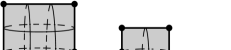
Figure 14. Pillowcase cover (on the left) over the pillowcase orbifold (on the right). A general pillowcase cover it is not necessarily glued from two identical polygons.

Consider a connected ramified cover $\hat{\mathcal{P}}$ over $\mathcal{P}$ of degree $N$ having ramification points only over the corners of the pillowcase. Clearly, $\hat{\mathcal{P}}$ is tiled by $2N$ squares of the size $(1/2)\times(1/2)$ in such way that the squares do not superpose and the vertices are glued to the vertices. Coloring the two squares of the pillowcase $\mathcal{P}$ one in black and the other in white, we get a chessboard coloring of the square tiling of the cover $\hat{\mathcal{P}}$: the white squares are always glued to the black ones and vice versa.

Lemma B.1.

Let $S$ be a flat surface in the stratum ${\mathcal{Q}}(d_{1},\dots,d_{k})$. The following properties are equivalent:

1. The surface $S$ represents a lattice point in ${\mathcal{Q}}(d_{1},\dots,d_{k})$;

2. $S$ is a cover over $\mathcal{P}$ ramified only over the corners of the pillow;

3. $S$ is tiled by black and white $(1/2)\times(1/2)$ squares respecting the chessboard coloring.

Proof.

We have just proved that (2) implies (3). To prove that (1) implies (2) we define the following map from $S$ to $\mathcal{P}$. Fix a zero or a pole $P_{0}$ on $S$. For any $P\in S$ consider a path $\gamma(P)$ joining $P_{0}$ to $P$ having no self-intersections and having no zeroes or poles inside. The restriction of the quadratic differential $q$ to such $\gamma(P)$ admits a well-defined square root $\omega=\pm\sqrt{q}$, which is a holomorphic form on the interior of $\gamma$. Define

(B.2) $$P\mapsto\left(\int_{\gamma(P)}\omega\mod\mathbb{Z}\oplus i\mathbb{Z}\right)/\pm\,.$$

Of course, the path $\gamma(P)$ is not uniquely defined. However, since the flat surface $S$ represents a lattice point (see the definition in  §4.1), the difference of the integrals of $\omega$ over any two such paths $\gamma_{1}(P)$ and $\gamma_{2}(P)$ belongs to $\mathbb{Z}\oplus i\mathbb{Z}$, so taking the quotient over the integer lattice and over $\pm$ we get a well-defined map. By definition of the pillowcase $\mathcal{P}$ we have, $\mathcal{P}=\left({\mathbb{C}}/(\mathbb{Z}\oplus i\mathbb{Z})\right)/\pm$. Thus, we have defined a map $S\to\mathcal{P}$. It follows from the definition of the map, that it is a ramified cover, and that all regular points of the flat surface $S$ are regular points of the cover. Thus, all ramification points are located over the corners of the pillowcase.

A similar consideration shows that (3) implies (1). ∎

Let $\operatorname{Sq}_{N}(d_{1},\dots,d_{k})$ be the number of surfaces in the stratum ${\mathcal{Q}}(d_{1},\dots,d_{k})$ tiled with at most $N$ black and $N$ white squares respecting the chessboard coloring. Lemma B.1 allows us to rewrite formula (B.1) as follows:

$$\mu(C({\mathcal{Q}}_{1}(d_{1},\dots,d_{k}))=\lim_{N\to+\infty}N^{-\dim_{{\mathbb{C}}}{\mathcal{Q}}(d_{1},\dots,d_{k})}\cdot\operatorname{Sq}_{N}(d_{1},\dots,d_{k})\,.$$

Taking into consideration (4.5) we get

(B.3) $$\operatorname{Vol}{\mathcal{Q}}_{1}(d_{1},\dots,d_{k})=2\dim_{\mathbb{C}}{\mathcal{Q}}(d_{1},\dots,d_{k})\,\cdot\\ \lim_{N\to+\infty}N^{-\dim_{{\mathbb{C}}}{\mathcal{Q}}(d_{1},\dots,d_{k})}\cdot\operatorname{Sq}_{N}(d_{1},\dots,d_{k})\,.$$

We now state and prove two Lemmas which we use in the proof of Theorem 1.3.

Lemma B.2.

For any $\eta,\nu$ as above the following asymptotic relation is valid:

(B.4) $$\lim_{N\to+\infty}\frac{\sum_{d=1}^{N}\operatorname{Cov}^{0}_{4d}(\eta,\nu)}{\sum_{d=1}^{N}\operatorname{Cov}^{0,{\scriptscriptstyle\boxplus}}_{4d}(\eta,\nu)}=2^{\ell(\eta)}\,,$$

where $\ell(\eta)$ is the number of entries in $\eta$.

Proof.

Let $P$ be a zero of even degree of a quadratic differential, and $U_{\varepsilon}(P)$ a multidisc of flat radius $\varepsilon$ centered at $P$. Choosing $\varepsilon$ sufficiently small, we can assume that $U_{\varepsilon}(P)$ is embedded into the ambient flat surface. (For example, for the flat surface $\hat{\mathcal{P}}$ induced from the standard $\frac{1}{2}\times\frac{1}{2}$ square pillowcase $\mathcal{P}$ by means of the cover $\pi_{\scriptscriptstyle\boxplus}:\hat{\mathcal{P}}\to\mathcal{P}$ one can choose any $\varepsilon$ satisfying $0<\varepsilon<\frac{1}{2}$.) Choose an orientation of the vertical direction in $U_{\varepsilon}(P)$. For any vector $\vec{v}\in{\mathbb{R}}^{2}$ such that $\|\vec{v}\|<\varepsilon$ there is a unique way to move the zero $P$ in direction $\vec{v}$ by the distance $\|\vec{v}\|$ via a local move inside $U(P)$ keeping the flat metric outside of $U(P)$ unchanged. The corresponding local surgery (called,

Figure 15. Cartoon of a local move of a zero of even degree.

depending on the author and the context Schiffer variation, or deformation along the kernel (or Rel) foliation, etc) is represented in Figure 15, where the separatrix rays (“prongs”) adjacent to $P$ are chosen to be parallel to the vector $\vec{v}$. This local deformation can be performed as follows. Make short slits along all prongs in direction $\vec{v}$ and open them. The original conical point of a cone angle $\pi\cdot 2k$ gives rise to $2k$ marked points on the sides of the slits. Move the marked points along the sides of the slit by the distance $\|\vec{v}\|$ in direction $\vec{v}$ and zip the slits back up to the new marked points. All new marked points get identified into a single conical singularity with the cone angle $\pi\cdot 2k$. Note that usually, the flat surfaces obtained after deformations along vectors $\vec{v}$ and $-\vec{v}$ are generically non-isomorphic.

Consider now a pillowcase cover $\pi_{\scriptscriptstyle\boxplus}:\hat{\mathcal{P}}\to\mathcal{P}$ as above. As the base sphere choose the standard pillowcase $\mathcal{P}$ endowed with the quadratic differential $q_{0}=(dz)^{2}$. It has four simple poles at the corners of the pillow and no other singularities. Pulling back $(dz)^{2}$ via $\pi_{\scriptscriptstyle\boxplus}$ gives a quadratic differential on the covering ${\mathbb{C}}\!\operatorname{P}^{1}$ with zeros and simple poles of degrees $\{\nu_{i}-2\}$ and $\{2\eta_{j}-2\}$ and with no other singularities. Thus, by construction the pillowcase cover $\hat{\mathcal{P}}:=({\mathbb{C}}\!\operatorname{P}^{1},\pi^{\ast}q_{0})$ belongs to ${\mathcal{Q}}(\eta,\nu)$.

Move the zero $P_{1}$ of degree $2\eta_{1}-2$ in direction $\vec{v}$ as above. The deformed flat surface inherits a structure of a ramified cover over the pillowcase orbifold $\mathcal{P}$. The corresponding cover can be defined by a formal construction as equation (B.2), or can be seen in plain terms as follows. We have deformed our flat structure only inside a neighborhood $U(P_{1})$, so we let the projection of the complement of $U(P_{1})$ to the pillowcase orbifold $\mathcal{P}$ unchanged. The neighborhood $U(P_{1})$ is glued from even number $2k$ of half-disks as in Figure 15; we define the projection of each half-disk to the pillowcase orbifold $\mathcal{P}$ unchanged.The definition matches on the common boundaries of the half-discs. By construction, the deformed cover $\pi^{\prime}:\hat{\mathcal{P}}^{\prime}\to\mathcal{P}$, has the ramification profile $(2\eta_{2},\dots,2\eta_{\ell(\eta)},\nu,2^{2d-|\eta|+\eta_{1}-|\nu|/2})$ over $0\in\mathcal{P}$, profile $(\eta_{1},1^{4d-\eta_{1}})$ over the projection of the deformed zero $P_{1}^{\prime}$, and profile $(2^{2d})$ over the other three corners of $\mathcal{P}$. The cover $\pi^{\prime}$ is unramified elsewhere.

Consider now the same pillowcase cover $\pi_{\scriptscriptstyle\boxplus}:\hat{\mathcal{P}}\to\mathcal{P}$ as above and move the zero $P_{1}$ of degree $2\eta_{1}-2$ of the initial quadratic differential $q$ in direction $-\vec{v}$. Clearly we get a pillowcase cover $\pi^{\prime\prime}:\hat{\mathcal{P}}^{\prime\prime}\to\mathcal{P}$ with exactly the same profile as $\pi^{\prime}:\hat{\mathcal{P}}^{\prime}\to\mathcal{P}$. Moreover, since the zero $P_{1}$ of $q$ on the original cover $\hat{\mathcal{P}}$ was projected to a conical singularity of the pillowcase orbifold $\mathcal{P}$ with the cone angle $\pi$, moving from the corresponding corner of the pillow in directions $\vec{v}$ and $-\vec{v}$ we get to the same point of the pillowcase orbifold $\mathcal{P}$. In other words, the zero $P_{1}^{\prime}$ of the deformed quadratic differential $q^{\prime}$ on $\hat{\mathcal{P}}^{\prime}$ obtained by moving the zero $P_{1}$ of $q$ in direction $\vec{v}$ is projected to the same point of the pillowcase orbifold $\mathcal{P}$ as the zero $P_{1}^{\prime\prime}$ of $q^{\prime\prime}$ on $\hat{\mathcal{P}}^{\prime\prime}$ obtained by moving the zero $P_{1}$ of $q$ in direction $-\vec{v}$. The number of covers $\hat{\mathcal{P}}$ for which the resulting covers $\hat{\mathcal{P}}^{\prime}$ and $\hat{\mathcal{P}}^{\prime\prime}$ are isomorphic has asymptotics of lower order in $N$ than $\sum_{d=1}^{N}\operatorname{Cov}^{0}_{4d}(\eta,\nu)$.

Moving all even-order zeroes $P_{1},\dots,P_{\ell(\eta)}$ in directions of pairwise-distinct vectors $\pm\vec{v}_{1},\dots,\pm\vec{v}_{\ell(\eta)}$ we establish a $2^{\ell(\eta)}$-to-one correspondence (up to a term of lower order asymptotics in $N$) between covers $\pi$ and $\pi_{\scriptscriptstyle\boxplus}$. ∎

Quadratic differentials induced from $dz^{2}$ on the standard pillowcase orbifold via the pillowcase covers (1.5) constructed in §1.2 have the following structure. All zeroes of odd degrees of such differentials are projected to the same corner of the pillow, while all zeroes of even degrees are projected to pairwise distinct non-corner points. Quadratic differentials induced from $dz^{2}$ on the standard pillowcase orbifold via the pillowcase covers $\pi_{\scriptscriptstyle\boxplus}:\hat{\mathcal{P}}\to\mathcal{P}$ as above have slightly different structure. Namely, all their zeroes (no matter of odd or even degree) project to the same corner of the pillowcase orbifold, so they are really square-tiled. Moreover, since all preimages under $\pi_{\scriptscriptstyle\boxplus}$ of the three remaining corners of the pillowcase orbifold are regular points of the flat metric, the resulting flat surface $\hat{\mathcal{P}}$ can be tiled with $1\times 1$ squares (compared to $\frac{1}{2}\times\frac{1}{2}$ squares of the pillowcase orbifold). Our next Lemma proves, that (in genus zero) this new square tiling with larger squares admits a chessboard coloring.

Lemma B.3.

Any pillowcase cover $\pi_{\scriptscriptstyle\boxplus}:\hat{\mathcal{P}}\to\mathcal{P}$ of genus zero with a ramification profile as above decomposes into two consecutive covers

$$\pi:\hat{\mathcal{P}}\rightarrow\mathcal{P}_{4}\rightarrow\mathcal{P}\,,$$

where $\mathcal{P}_{4}\rightarrow\mathcal{P}$ is a cover of order $4$ of a pillowcase orbifold of size $1\times 1$ over the standard pillowcase of size $\frac{1}{2}\times\frac{1}{2}$.

Remark B.4.

Without the condition that the genus of $\hat{\mathcal{P}}$ as above is equal to zero the assertion of Lemma B.3 is no longer true in general.

Proof of Lemma B.3.

Consider the decomposition of $\hat{\mathcal{P}}$ into maximal horizontal cylinders. We associate to this decomposition a finite graph. The edges of the graph are in one-to-one correspondence with the cylinders. The vertices of the graph are in one-to-one correspondence with connected components of singular horizontal layers. Two edges have common vertex if the corresponding maximal cylinders are adjacent to the same connected component of the critical horizontal layer.

Note, that for square-tiled surfaces of genus zero the resulting graph is, actually, a tree which we denote by $\operatorname{T}$. To prove the Lemma we first prove that perimeters of all horizontal cylinders are even integer numbers. The proof is an induction in the number of horizontal cylinders.

The base of induction corresponds to the case when $\hat{\mathcal{P}}$ has a single horizontal cylinder. Then $\hat{\mathcal{P}}$ has only two singular layers, one on each side of the cylinder. Consider one of the horizontal singular layers as a graph of horizontal saddle connections. Since $\hat{\mathcal{P}}$ is a sphere, the corresponding graph is, actually, a tree. By construction each saddle connection has integer length. The waist curve of the cylinder follows each saddle connection twice, so its perimeter is twice the sum of lengths of all saddle connections in the layer, and hence the perimeter is an even number.

When the number of horizontal cylinders is greater than one, analogous consideration shows that perimeters of all cylinders represented by the extremity edges (leaves) of the tree $\operatorname{T}$ have even perimeters. Chopping one of these cylinders out from the initial flat surface $\hat{\mathcal{P}}$ and isometrically identifying the parts of the boundary in the natural way we get a new pillowcase cover $\tilde{\mathcal{P}}$ satisfying the same properties as before. By induction all its horizontal cylinders have even perimeters.

Having proved that the perimeters of all horizontal cylinders are even integers we apply the induction in the number of cylinders one more time proving now that the tiling of $\hat{\mathcal{P}}$ with $1\times 1$ squares admits chessboard coloring. ∎

Now everything is ready to prove Theorem 1.3.

Proof of Theorem 1.3.

By Lemma B.3 a pillowcase cover $\pi_{\scriptscriptstyle\boxplus}:\hat{\mathcal{P}}\to\mathcal{P}$ of genus zero and of degree $4d$ with ramification data $(\eta,\nu)$ as above uniquely defines a square-tiled pillowcase cover of degree $d$ in ${\mathcal{Q}}(\eta,\nu)$.

Reciprocally, consider an arbitrary square-tiled surface $S$ as in Lemma B.1 above in the stratum ${\mathcal{Q}}(\eta,\nu)$, and let $d$ be the degree of the corresponding cover over $\mathcal{P}$. Subdividing each square into four; considering the underlying pillowcase as $\mathcal{P}_{4}$ and postcomposing the initial cover $S\to\mathcal{P}_{4}$ with the cover $\mathcal{P}_{4}\to\mathcal{P}$ we get a pillowcase cover with singularity pattern $(\eta,\nu)$. This implies that

$$\sum_{d=1}^{N}\operatorname{Cov}^{0,{\scriptscriptstyle\boxplus}}_{4d}(\eta,\nu)=\operatorname{Sq}_{N}(\nu_{1}-2,\nu_{2}-2,\dots,2\eta_{1}-2,2\eta_{2}-2,\dots)\,.$$

Applying equation (B.4) from Lemma B.2, taking into consideration that

$$\dim_{{\mathbb{C}}}{\mathcal{Q}}(\nu_{1}-2,\nu_{2}-2,\dots,2\eta_{1}-2,2\eta_{2}-2,\dots)=\ell(\nu)+\ell(\eta)-2$$

and applying equation (B.3) we complete the proof of Theorem 1.3. ∎

C. Equidistribution of Circle Translates
by Jon Chaika

We use a variation of an argument of G. A. Margulis to obtain equidistribution of circles from exponential mixing of the Teichmüller geodesic flow on ${\mathcal{Q}}_{1}$. The strategy is similar in spirit to [EMaMo98, Section 3.6].

C.1. Notation

As in §1.3, let ${\mathcal{B}}={\mathcal{B}}(k_{1},\dots,k_{n})$ be the space of directional billiard tables, that is, billiard tables with interior angles $(\tfrac{\pi}{2}k_{1},\dots,\tfrac{\pi}{2}k_{n})$ and a distinguished direction. ${\mathcal{B}}$ has the natural the measure $\mu_{\mathcal{B}}$ which is the product measure of the Lebesgue measure arising from the side lengths and the angular measure $d\phi$.

Given $\Pi\in{\mathcal{B}}$, let $q_{\Pi}$ be the meromorphic quadratic differential given by gluing together two copies of $\Pi$. Recall that $\Pi\mapsto q_{\Pi}$ from ${\mathcal{B}}$ to ${\mathcal{Q}}={\mathcal{Q}}(k_{1}-2,\dots,k_{n}-2)$ is a local embedding where ${\mathcal{Q}}(d_{1},\dots,d_{n})$ is the stratum of quadratic differentials with zeros of order $d_{1},\dots,d_{n}$. Using this map, we may view ${\mathcal{B}}$ as a subset of ${\mathcal{Q}}$. Let ${\mathcal{Q}}_{1}\subset{\mathcal{Q}}$ denote the subset of surfaces of flat area $1/2$ (see Convention 4.1), and let $\mu_{1}=\mu_{{\mathcal{Q}}_{1}}$ denote the Masur-Veech measure on ${\mathcal{Q}}_{1}$. Let ${\mathcal{B}}_{1}$ denote the intersection of ${\mathcal{B}}\subset{\mathcal{Q}}$ with ${\mathcal{Q}}_{1}$. We abuse notation by denoting the restriction of the measure $\mu_{\mathcal{B}}$ to ${\mathcal{B}}_{1}$ again by $\mu_{{\mathcal{B}}}$. Let $\tilde{{\mathcal{B}}}_{1}$ denote the subset of ${\mathcal{B}}_{1}$ where the direction of the flow is parallel to one of the sides, and let $\mu_{\tilde{{\mathcal{B}}}}$ be the restriction of the measure to $\tilde{{\mathcal{B}}}_{1}$. We recall notation for important one-parameter subgroups of $SL(2,{\mathbb{R}})$:

$$g_{t}=\left(\begin{array}[]{cc}e^{t}&0\\ 0&e^{-t}\end{array}\right)\mbox{ and }r_{\theta}=\left(\begin{array}[]{cc}\cos\theta&\sin\theta\\ -\sin\theta&\cos\theta\end{array}\right)$$

C.2. Equidistribution

We define the function space

$$\mathcal{L}_{c}^{0}:=\left\{f\in C_{c}({\mathcal{Q}}_{1}):f\mbox{ is }1\mbox{-Lipschitz },\int_{{\mathcal{Q}}_{1}}fd\mu_{1}=0\right\}$$

with respect to the Euclidean metric induced by local coordinates on ${\mathcal{Q}}_{1}$ (see, for example [AG, §5] for a formal definition of this distance). We denote $\mathcal{L}_{c}$ the space without the mean $0$ condition.

Theorem C.1.

Let $f\in\mathcal{L}_{c}^{0}$. Then for $\mu_{\mathcal{B}}$-almost every right angled billiard $q_{\Pi}$ we have

$$\underset{T\to\infty}{\lim}\frac{1}{2\pi}\int_{0}^{2\pi}f(g_{T}r_{\theta}q_{\Pi})\,d\theta=\frac{1}{\mu_{1}({\mathcal{Q}}_{1})}\int_{{\mathcal{Q}}_{1}}f\,d\mu_{1}=0\,.$$

C.3. Small arcs and strategy

The strategy to prove Theorem C.1 is to break the integral over the circle into (exponentially) small arcs so that the limit converges as desired. Let $\mathcal{M}_{\varepsilon}\subset{\mathcal{Q}}_{1}$ be the $\varepsilon$-thick part of the stratum, that is, the set of $q\in{\mathcal{Q}}_{1}$ so that all saddle connections on $q$ have length at least $\varepsilon$.

Proposition C.2.

Let $f\in\mathcal{L}_{c}^{0}$ and $\delta>0$. Define

$$S_{\delta}:=\left\{\theta\in[0,2\pi)\setminus\left(B\left(0,\delta\right)\cup B\left(\frac{\pi}{2},\delta\right)\cup B\left(\pi,\delta\right)\cup B\left(\frac{3\pi}{2},\delta\right)\right)\right\}.$$

$S_{\delta}$ avoids neighborhoods of directions parallel to the sides. There exists an exponentially decaying function $v:\mathbb{R}^{+}\to[0,\pi)$ such that for any $\varepsilon>0$

$$\lim_{N\rightarrow\infty}\frac{1}{2v(\varepsilon N)}\int_{-v(\varepsilon N)}^{v(\varepsilon N)}f(g_{\varepsilon N}r_{\theta+\phi}q_{\Pi})d\phi=\frac{1}{\mu_{1}({\mathcal{Q}}_{1})}\int_{{\mathcal{Q}}_{1}}fd\mu_{1}$$

for $\mu_{\mathcal{B}}$-almost every $q_{\Pi}\in\tilde{{\mathcal{B}}_{1}}\cap\mathcal{M}_{\delta}$, Lebesgue almost every $\theta\in S_{\delta}$.

We prove Theorem C.1 assuming Proposition C.2 in §C.7. To prove Proposition C.2, we estimate the $L^{2}$-norms of the functions

$$F_{N}(q)=\frac{1}{2v(N)}\int_{-v(N)}^{v(N)}f(g_{N}r_{\theta}q)d\theta,$$

on $\mathcal{M}_{\delta}\cap r_{\theta}\tilde{\mathcal{B}_{1}}$, the $\delta$-thick part of the rotated billiard subvariety. To estimate

$$\int_{r_{\theta}\tilde{{\mathcal{B}}_{1}}\cap\mathcal{M}_{\delta}}(F_{N}(q))^{2}\,d\mu_{r_{\theta}\mathcal{B}}=\int_{r_{\theta}\tilde{{\mathcal{B}}_{1}}\cap\mathcal{M}_{\delta}}\frac{1}{4v(N)^{2}}\int_{-v(N)}^{v(N)}\int_{-v(N)}^{v(N)}(g_{N}r_{x}q)f(g_{N}r_{y}q)\,dx\,dy\,d\mu_{r_{\theta}\mathcal{B}},$$

we separate the domain of integration into two pieces: one where $x$ and $y$ are very close, and another when they are sufficiently separated. Heuristically, for $x$ and $y$ sufficiently separated, the translates $g_{N}r_{x}q$ and $g_{N}r_{y}q$ move away from each other exponentially in $N$, and thus become uncorrelated due to exponential mixing of the Teichmüller flow. This is made precise in Proposition C.10. For $x$ and $y$ sufficiently close, we estimate trivially by the measure of the set.

C.4. Exponential recurrence, mixing, and contraction

To implement the above strategy, we need three crucial technical results on Teichmüller geodesic flow.

C.4.1. Exponential Recurrence

Athreya [At06] showed that most (in an exponential sense) trajectories spend at least half their life in the thick part of a stratum. Precisely, let

$$G_{L}(\varepsilon)=\left\{q\in{\mathcal{Q}}_{1}:\left|\left\{0\leq t<T:g_{t}q\in\mathcal{M}_{\varepsilon}\right\}\right|>\frac{T}{2}\text{ for all }T>L\right\}$$

denote the set of $q\in{\mathcal{Q}}_{1}$ so that the $g_{t}$-trajectory of $q$ eventually (after time $L$) spends at least half its life in $\mathcal{M}_{\varepsilon}$.

Theorem C.3 ([At06, Theorem 2.3]).

For all small enough $\varepsilon>0$, there exists $C,\xi>0$ such that for all $L>0$

$$\mu_{1}(G_{L}(\varepsilon))>(1-Ce^{-\xi L})\mu_{1}({\mathcal{Q}}_{1}).$$

C.4.2. Exponential Mixing

Avila-Resende [AR12], building on work of Avila-Gouezel-Yoccoz [AGY], showed that the Teichmüller geodesic flow is exponentially mixing. Let $d$ be the Riemannian distance on $\operatorname{SL}(2,{{\mathbb{R}}})$ induced by the Killing form. For functions $f,g$ on ${\mathcal{Q}}_{1}$, and $M\in SL(2,{\mathbb{R}})$, define the $M$-correlation

$$\mathcal{C}(f,g,M)=\left|\int_{\mathcal{Q}_{1}}f(Mq)g(q)d\mu_{1}-\int_{\mathcal{Q}_{1}}fd\mu_{1}\int_{\mathcal{Q}_{1}}gd\mu_{1}\right|$$

Theorem C.4.

([AR12], [AGY, Theorem 2.14]) There exists constants $C,\lambda$ so that if $h_{1},h_{2}$ are Lipshitz and compactly supported then there exists $C_{K}$ that depend only on the smallest systole of a surface in the compact support such that for any $M\in SL(2,{\mathbb{R}})$,

$$\mathcal{C}(h_{1},h_{2},M)\leq\\ C\left(C_{K}+\|h_{1}\|_{\infty}+\|h_{1}\|_{Lip}\right)\left(C_{K}+\|h_{2}\|_{\infty}+\|h_{2}\|_{Lip}\right)e^{-\lambda d(M,id)}.$$

C.4.3. Exponential Contraction

Eskin-Mirzakhani-Rafi [EMR], following Forni [Fo01], proved an important result on the hyperbolicity of the Teichmüller flow. For a subset $A\subset{\mathbb{R}}^{n}$ we use $|A|$ to denote its Lebesgue measure.

Theorem C.5 ([EMR, Lemma 8.3]).

Given a fixed compact part $\mathcal{M}_{\frac{\varepsilon}{2}}$ there exists $c,\tilde{C}>0$ such that if $q$ and $q^{\prime}$ differ only along a stable manifold for $g_{t}$ (that is, if they share the same horizontal foliation) then

$$d_{S}(g_{t}q,g_{t}q^{\prime})<\tilde{C}d_{S}(q,q^{\prime})e^{-c\left|\left\{t>0:g_{t}q\in\mathcal{M}_{\frac{\varepsilon}{2}}\right\}\right|}.$$

$d_{S}$ denotes Hodge distance along the stable manifold. See [EMR, Section 8.2].

C.5. Mixing on open sets

In this section we state and prove our first key lemma Proposition C.6, which will play a crucial role in the proof of Proposition C.2. Proposition C.6 uses exponential mixing (Theorem C.4) in a crucial fashion.

Given an open set $U\subset\mathcal{M}_{\delta}$, let $\partial_{\varepsilon}U$ denote the $\varepsilon$-neighborhood of the boundary $\partial U$. We say $U$ is polynomially regular with regularity polynomial $P$ if there is a polynomial $P$ so that

$$\mu_{1}(\partial_{\varepsilon}U)\leq P(\varepsilon).$$

Proposition C.6.

Let $\delta>0$ and let $U\subset\mathcal{M}_{\delta}$ be polynomially regular. Let $f,h\in\mathcal{L}_{c}^{0}$. Then there exist $\hat{\lambda},D>0$ and $\ell_{0}<1$ so that for all $0<\ell<\ell_{0}$

$$\left|\int_{U}f(g_{t}q)h(g_{(1+\ell)t}q)d\mu_{1}(q)\right|\leq De^{-\hat{\lambda}\ell}.$$

Moreover, the constants only depend on $\delta$, $\|f\|_{\infty}$, $\|h\|_{\infty}$ and the regularity polynomial of $U$.

The first step in the proof is the following effective equidistribution lemma for translates of polynomially regular sets.

Lemma C.7.

Let $\delta>0$, $U\subset\mathcal{M}_{\delta}$ be polynomially regular and $f\in\mathcal{L}^{c}_{0}$. There exist $E,\lambda_{f}>0$ so that

$$\left|\frac{1}{\mu_{1}(U)}\int_{U}f(g_{t}q)d\mu_{1}(q)\right|\leq Ee^{-\lambda_{f}t}.$$

The constants depend only on $\delta,f$ and the regularity polynomial of $U$.

Proof.

Let $U_{r}=\{q\in U:B(q,r)\subset U\}$ and

$$h_{\varepsilon}(q)=\chi_{U}(q)\left(1-\frac{1}{\varepsilon}d(q,U_{\varepsilon})\right).$$

Notice that $h_{\varepsilon}$ is $\varepsilon^{-1}$-Lipshitz. We will obtain the lemma by applying exponential mixing (Theorem C.4) to the functions $f$ and $h_{\varepsilon}$.

$$\left|\int_{U}f(g_{t}q)d\mu_{1}\right|\leq\left|\int_{\mathcal{Q}_{1}}h_{\varepsilon}(q)f(g_{t}q)d\mu_{1}\right|+\|\chi_{U}-h_{\varepsilon}\|_{\infty}\mu_{1}\left\{q:\chi_{U}(q)\neq h_{\varepsilon}(q)\right\}\|f\|_{\infty}.$$

By Theorem C.4 we have that there exists $C_{3}$ (subsuming the various constants)

$$\left|\int_{\mathcal{Q}_{1}}h_{\varepsilon}(q)f(g_{t}q)d\mu_{1}\right|\leq C_{3}\frac{1}{\varepsilon}e^{-\lambda t}.$$

By our assumption on $U$ there exists $C,d$ (essentially the leading coefficient and degree of the regularity polynomial) so that

$$\|\chi_{U}-h_{\varepsilon}\|_{\infty}\mu_{1}\left\{q:\chi_{U}(q)\neq h_{\varepsilon}(q)\right\}\|f\|_{\infty}\leq C\varepsilon^{d}.$$

Letting $\varepsilon=e^{-\frac{\lambda}{4}t}$ we obtain

$$\int_{U}f(g_{t}q)d\mu_{1}\leq C_{\varepsilon,f}e^{\frac{\lambda}{4}t}e^{-\lambda t}+Ce^{-\frac{\lambda d}{4}t}.$$

To complete the lemma, let $\lambda_{f}=\min\left\{\frac{\lambda}{2},\frac{d\lambda}{4}\right\}$. ∎

Applying this to small balls, we obtain

Corollary C.8.

Let $\varepsilon>0$, $q_{0}\in\mathcal{M}_{\varepsilon+e^{-k}}$ and $f\in\mathcal{L}_{c}^{0}$. Then there exists $C_{k,\varepsilon,f}>0$ so that for all $k>0$,

$$\left|\frac{1}{\mu_{1}(B(q_{0},e^{-k})))}\int_{B(q_{0},e^{-k})}f(g_{t}q)d\mu_{1}(q)\right|\leq C_{k,\varepsilon,f}e^{-\lambda_{f}t}.$$

Moreover, $C_{k,\varepsilon,f}$ can be chosen to be $C_{\varepsilon,f}e^{kL_{\varepsilon,f}}$ where $L_{\varepsilon,f}$ depends only on $\varepsilon,f$.

Applying this corollary to $f=\chi_{U}-\mu_{1}(U)$ for a polynomially regular set, we obtain

Corollary C.9.

Let $\delta>0$. Let $U\subset\mathcal{M}_{\delta}$ be polynomially regular. There exist $k_{2},D_{2},\lambda_{2}$ so that for any $q_{0}\in\mathcal{M}_{\delta}$ we have, for all $r>0$

$$\left|\frac{1}{\mu_{1}(B(q_{0},e^{-r}))}\int_{B(q_{0},e^{-r})}\chi_{U}(g_{k_{2}r}q)d\mu_{1}(q)-\mu_{1}(U)\right|<D_{2}e^{-\lambda_{2}r}.$$

$k_{2}$ can be chosen to be either positive or negative and the corollary holds for all large enough (in absolute value) $k_{2}$. The constants can be chosen to only depend on $\delta$ and the regularity polynomial of $U$.

Proof.

Let

$$H_{r,q_{0}}(q)=\left(e^{2r}-1\right)d\left(q,B(q_{0},e^{-r})\right)\chi_{B\left(q_{0},e^{-r}+e^{-2r}\right)}\left(q\right).$$

By the regularity of $U$ and using period coordinates on the stratum we have that there exist $C^{\prime}_{1},d_{1}$ and $C_{2}^{\prime},d_{2}$ so that

$$\left|\int_{B(q_{0},e^{-r})}\chi_{U}(g_{kr}q)d\mu_{1}-\int_{{\mathcal{Q}}_{1}}h_{\varepsilon}(q)H_{r,q_{0}}(q)d\mu_{1}\right|<C^{\prime}_{1}\varepsilon^{d_{1}}+C^{\prime}_{2}e^{-2rd_{2}}.$$

By Theorem C.4, since

$$\|H_{r,q_{0}}\|_{Lip}\leq e^{2r}\mbox{ and }\|h_{\varepsilon}\|_{Lip}\leq\frac{1}{\varepsilon}$$

we have that there exists $C_{3}$ (subsuming the various constants) so that

$$\left|\int_{{\mathcal{Q}}_{1}}h_{\varepsilon}(g_{kr}q)H_{q_{0},r}(q)d\mu_{1}-\int H_{q,r}d\mu_{1}\int h_{\varepsilon}d\mu_{1}\right|<C_{3}\frac{1}{\varepsilon}e^{2r}e^{-\lambda k}.$$

Combining these two estimates the corollary follows. ∎

Note that if $f\in\mathcal{L}_{c}^{0}$ then $f\circ g_{t}$ is $Ce^{3t}$-Lipshitz. We use this observation to prove Proposition C.6 by splitting $U$ into balls of size $e^{-4t}$ where $f\circ g_{t}$ is basically constant. Then we apply Lemma C.8 to these balls. This gives us the required independence.

Proof of Proposition C.6.

We want to estimate

$$\left|\int_{U}f(g_{t}q)h(g_{t+s}q)d\mu_{1}(q)\right|=\left|\int_{{\mathcal{Q}}_{1}}f(q)h(g_{s}q)\chi_{U}(g_{-t}q)d\mu_{1}(q)\right|$$

By doing an extra integration over small balls, we rewrite this as

$$\left|\int_{{\mathcal{Q}}_{1}}\frac{1}{\mu_{1}(B(q_{0},e^{-4s}))}\int_{B(q_{0},e^{-4s})}f(q)h(g_{s}q)\chi_{U}(g_{-t}q)d\mu_{1}(q)d\mu_{1}(q_{0})\right|$$

Since $f,h\in\mathcal{L}_{c}^{0}$ we can estimate their values in small balls by values at the center points, allowing us to bound from above the previous integral by

$$\left|\int_{{\mathcal{Q}}_{1}}\frac{1}{\mu_{1}(B(q_{0},e^{-4s}))}\int_{B(q_{0},e^{-4s})}\left(f(q_{0})h(g_{s}q_{0})+O(e^{-4s})\|f\|_{Lip}\|h\circ g_{s}\|_{Lip}\right)\chi_{U}(g_{-t}q)d\mu_{1}(q)d\mu_{1}(q_{0})\right|$$

Integrating the error term out, we derive the further estimate

$$\left|\int_{{\mathcal{Q}}_{1}}\frac{1}{\mu_{1}(B(q_{0},e^{-4s}))}f(q_{0})h(g_{s}q_{0})\int_{B(q_{0},e^{-4s})}\chi_{U}(g_{-t}q)d\mu_{1}(q)d\mu_{1}(q_{0})\right|+O\left(e^{-\frac{3s}{4}}\right).$$

By Corollary C.9 if $s<\frac{t}{k_{2}}$ then for any $q_{0}$ in the support of $f$ (which is assumed to be compact)

$$\left|\frac{1}{\mu_{1}(B(q_{0},e^{-4s}))}\int_{B(q_{0},e^{-4s})}\chi_{U}(g_{-t}q)d\mu_{1}(q)-\mu_{1}(U)\right|<D_{2}e^{-\lambda_{2}s}.$$

So we obtain

(C.1) $$\left|\int_{{\mathcal{Q}}_{1}}\frac{1}{\mu_{1}(B(q_{0},e^{-4s}))}f(q_{0})h(g_{s}q_{0})\int_{B(q_{0},e^{-4s})}\chi_{U}(g_{-t}q)d\mu_{1}(q)d\mu_{1}(q_{0})\right|=\\ \left|\mu(U)\int_{{\mathcal{Q}}_{1}}f(q_{0})h(g_{s}q_{0})d\mu_{1}(q_{0})\right|+O\left(D_{2}e^{-\lambda_{2}s}\right)\|f\|_{\infty}\|h\|_{\infty}.$$

Applying Theorem C.4 Proposition C.6 follows. ∎

C.6. Correlation of translates

In this subsection, we state our other key lemma Proposition C.10, which estimates the correlation of $f\in\mathcal{L}_{c}^{0}$ with a translate of $f$ along a thickened $g_{t}$-translate of the billiard manifold $\tilde{\mathcal{B}_{1}}$. Fix $\varepsilon>0$ so that Theorem C.3 holds.

Proposition C.10.

If $f\in\mathcal{L}_{c}^{0}$, $\delta,a>0$ and $\theta\notin\{0,\frac{\pi}{2},\pi,3\frac{\pi}{2}\}$ then there exist constants $C_{1}^{\prime},\lambda^{\prime}$ and $C_{2,\theta}<1$ such that for any $M\in\operatorname{SL}(2,{{\mathbb{R}}})$ with $d(M,Id)\leq e^{tC_{2,\theta}}$ we have

$$\left|\int_{-a}^{a}\int_{r_{\theta}\tilde{\mathcal{B}_{1}}\cap\mathcal{M}_{\delta}}f(Mg_{t+\ell}q)f(g_{t+\ell}q)\,d\mu_{r_{\theta}\tilde{\mathcal{B}_{1}}}(q)d\ell\right|<C_{\theta}e^{-\lambda^{\prime}_{\theta}d(M,Id)}.$$

Here, and below, $\mu_{r_{\theta}{\mathcal{B}}_{1}}$ denotes $(r_{\theta})_{*}\mu_{\tilde{{\mathcal{B}}_{1}}}$. $C_{\theta},C_{2,\theta}$ and $\lambda^{\prime}_{\theta}$ depend on $f$, $\delta$, $a$ and $\theta$. Moreover fixing $f,a,\delta$ the dependence on $\theta$ is continuous.

The proof of Proposition C.10 relies on all of the technical ingredients from the previous sections: exponential recurrence (Theorem C.3) exponential mixing (Theorem C.4) and exponential contraction (Theorem C.5) as well as Proposition C.6. Our key lemma is:

Lemma C.11.

Let $\delta>0$ and $U\subset\mathcal{M}_{\delta}$ be polynomially regular. Let $f,h\in\mathcal{L}_{c}^{0}$. Then there exist constants $\hat{C},C_{2},\lambda$ such that for any $M\in\operatorname{SL}(2,{{\mathbb{R}}})$ with $\|M\|<C_{2}t$ we have

$$\left|\int_{U}f(g_{t}q)h(Mg_{t}q)\,d\mu_{1}(q)\right|<\hat{C}e^{-\lambda d(M,Id)}.$$

As in Proposition C.6, $\hat{C}$ and $\lambda$ depend on $f,h,\delta$ and the regularity polynomial of $U$.

Proof.

There exist $\theta,\phi\in S^{1}$, $s\in\mathbb{R}$ with $e^{s}=\|M\|$ so that $M=r_{\theta}g_{s}r_{\phi}$.

$$\int_{U}f(g_{t}q)h(Mg_{t}q)\,d\mu_{1}(q)=\int_{Q}f(q)h(r_{\theta}g_{s}r_{\phi}q)\chi_{U}(g_{-t}q)d\mu_{1}(q)=\\ \int_{{\mathcal{Q}}_{1}}(f\circ r_{-\phi}(q))(h\circ r_{\theta}(g_{s}q))\chi_{U}(g_{-t}r_{-\phi}q)d\mu_{1}(q).$$

We now follow the approach of the proof of Proposition C.6 and for convenience introduce $h_{\theta}=h\circ r_{\theta},f_{\phi}=f\circ r_{-\phi}\in\mathcal{L}_{c}^{0}$.

$$\left|\int_{{\mathcal{Q}}_{1}}\frac{1}{\mu_{1}(B(q,e^{-4s}))}\int_{B(q,e^{-4s})}f_{\phi}(\omega)h_{\theta}(g_{s}\omega)\chi_{U}(g_{-t}r_{-\phi}\omega)d\mu_{1}(\omega)d\mu_{1}(q)\right|=\\ \left|\int_{{\mathcal{Q}}_{1}}\frac{1}{\mu_{1}(B(q,e^{-4s}))}f_{1}(q)h_{1}(g_{s}q)\int_{B(q,e^{-4s})}\chi_{U}(g_{-t}r_{-\phi}\omega)d\mu_{1}(\omega)d\mu_{1}(q)\right|+O\left(e^{-\frac{3s}{4}}\right).$$

Now

$$\left|\frac{1}{\mu_{1}(B(q,e^{-4s}))}\int_{B(q,e^{-4s})}\chi_{U}(g_{-t}r_{-\phi}\omega)d\mu_{1}(\omega)-\mu_{1}(U)\right|=\\ \left|\frac{1}{\mu_{1}(B(q,e^{-4s}))}\int_{r_{-\phi}B(q,e^{-4s})}\chi_{U}(g_{-t}\omega)d\mu_{1}(\omega)-\mu_{1}(U)\right|<D_{2}e^{-\lambda_{2}s}$$

since $r_{-\phi}B(q,e^{-4s})$ has the same regularity polynomial as $B(q,e^{-4s})$. This implies the lemma. ∎

Proof of Proposition C.10.

Let $\theta\notin\{0,\frac{\pi}{2},\pi,\frac{3\pi}{2}\}$. Intersect $r_{\theta}\tilde{\mathcal{B}}_{1}$ with $\mathcal{M}_{\varepsilon}$ and flow it by a small interval $\{g_{\ell},|\ell|<a\}$, and consider

$$\bigcup_{|\ell|<a}g_{\ell}r_{\theta}\tilde{\mathcal{B}}_{1}\cap\mathcal{M}_{\varepsilon}.$$

Thicken it by $c^{\prime}>0$ along the stable manifold for $g_{t}$, and call the resulting set $V$. We pick $a$ and $c^{\prime}$ small enough so that the intersection of $V$ with the support of $f$ has a local product structure (as stable $\times$ unstable $\times$ flow) with respect to the Teichmüller flow $g_{t}$. By the continuity of the trigonometric functions in the proof of Proposition 3.2 $a$ and $c^{\prime}$ can be chosen to depend continuously on $\theta$. Let $\Phi$ denote the local projection from $V$ to the $a$-thickened and $\theta$-rotated billiard subvariety

$$\bigcup_{|\ell|<a}g_{\ell}r_{\theta}\tilde{\mathcal{B}_{1}}.$$

By Proposition 3.2,

$$\mu_{1}(V)>0.$$

By Corollary C.11, if $\|M\|_{op}<\hat{C}_{2,\theta}$ we have that

$$\left|\int_{V\cap G_{t}}f(Mg_{t}q)f(g_{t}q)\,d\mu_{1}\right|\leq\hat{C}_{\theta}e^{-\lambda_{\theta}d(M,Id)}+\mu_{1}(G_{t}^{c}).$$

By the continuity of $r_{\theta}$ and the construction of $V$ the polynomial that bounds the decay of an $\varepsilon$ neighborhood of the boundary of $V$ can be chosen to depend continuously on $\theta$. So $\hat{C}_{\theta}$ and $\lambda_{\theta}$ depend continuously on $\theta$. By exponential recurrence (Theorem C.3) $\mu_{1}(G_{t}^{c})$ decays exponentially in $t$ and so there exists $C^{\prime\prime}_{\theta},\lambda^{\prime\prime}_{\theta}$ such that

$$\left|\int_{V\cap G_{t}}f(Mg_{t}q)f(g_{t}q)\,d\mu_{1}\right|\leq C^{\prime\prime}_{\theta}e^{-\lambda^{\prime\prime}_{\theta}d(M,Id)}.$$

Now for each $q\in V$ there exists $q^{\prime}\in r_{\theta}\tilde{\mathcal{B}_{1}}$ on the same stable manifold which is distance at most $c^{\prime}$ away. It follows from the exponential contraction of $g_{t}$ (Theorem C.5) that for $t$ large enough and $q^{\prime}\in G_{t}$ then

$$d(g_{t}q,g_{t}q^{\prime})<\tilde{C}c^{\prime}e^{-\frac{c}{2}t}.$$

By our assumption that $f\in\mathcal{L}_{c}^{0}$ it follows that

$$\left|f(g_{t}q)-f(g_{t}q^{\prime}\right)|<\tilde{C}c^{\prime}e^{-\frac{c}{2}t}$$

and

$$|f(Mg_{t}q)-f(Mg_{t}q^{\prime})|\leq\|M\|_{op}\tilde{C}c^{\prime}e^{-\frac{c}{2}t},$$

where $\|\cdot\|_{op}$ denotes the operator norm of $\operatorname{SL}(2,{{\mathbb{R}}})$ acting linearly on ${\mathbb{R}}^{2}$. By our assumption on $V$ and the fact that $f$ is 1-Lipschitz it follows that

$$\left|\int_{V\cap G_{t}}f(Mg_{t}q)f(g_{t}q)d\mu_{1}(q)\right|\geq\\ \left|\int_{V\cap G_{t}}f\left(Mg_{t}\Phi(q)+e_{q}\right)\left(f(g_{t}\Phi(q)+e^{\prime}_{q}\right)d\mu_{1}(q)\right|\geq\\ \left|\int_{[0,c^{\prime}]^{k}}\int_{-a}^{a}\int_{r_{\theta}\tilde{\mathcal{B}_{1}}\cap\mathcal{M}_{\frac{\varepsilon}{2}}}\left(f(Mg_{\ell+t}q^{\prime})+e_{q^{\prime},\ell,s}\right)\left(f(g_{t+\ell}q^{\prime})+e^{\prime}_{q^{\prime},\ell,s}\right)d\mu_{r_{\theta}\tilde{\mathcal{B}}}(q^{\prime})d\ell d\lambda^{k}(s)\right|+\zeta e^{-\xi t}\,,$$

where

$$|e^{\prime}_{q}|,|e^{\prime}_{q^{\prime},s}|<\tilde{C}c^{\prime}e^{-\frac{c}{2}t}\mbox{ and }|e_{q}|,|e_{q^{\prime},s}|<\|M\|_{op}\tilde{C}c^{\prime}e^{-\frac{c}{2}t}.$$

In the last inequality of the integral estimate, $\zeta e^{-\xi t}$ comes from the exponential recurrence result Theorem C.3. This establishes the Proposition. ∎

C.7. Proof of Theorem C.1

We prove our main Theorem C.1 assuming our key tool Proposition C.2. By Proposition C.2, for every $\delta>0$ there exists a $T_{0}$ such that for any $T>T_{0}$, $T\in\varepsilon\mathbb{N}$ and set $S$ with

$$\mu_{\mathcal{B}}(S)\geq\mu_{\mathcal{B}}(\mathcal{B}_{1}\cap\mathcal{M}_{\delta})-\delta$$

we have that for each $q\in S$ a subset $G_{q}$ of $S_{\delta}$ with

$$\lambda(G_{q})\geq 2\pi-8\delta-\delta$$

such that for each $\theta\in G_{q}$ we have

$$\left|\frac{1}{2v(T)}\int_{-v(T)}^{v(T)}f(g_{T}r_{\theta+\phi}q)d\phi\right|<\delta.$$

It follows that for $q\in S$ and $T>T_{0}$ we have

$$\left|\frac{1}{2\pi}\int_{0}^{2\pi}f(g_{T}r_{\phi}q)\,d\phi\right|=\left|\frac{1}{2\pi}\int_{0}^{2\pi}\frac{1}{2v(T)}\int_{-v(T)}^{v(T)}f(g_{T}r_{\theta+\phi}q)d\phi d\theta\right|$$

We break this integral into two pieces, over $G_{q}$ and its complement. We have

$$\left|\frac{1}{2\pi}\int_{G_{q}}\frac{1}{2v(T)}\int_{-v(T)}^{v(T)}f(g_{T}r_{\theta+\phi}q)d\phi d\theta\right|\leq\delta$$

and

$$\left|\int_{G_{q}^{c}}\frac{1}{2v(T)}\int_{-v(T)}^{v(T)}f(g_{T}r_{\theta+\phi}q)d\phi d\theta\right|\leq 9\delta\|f\|_{\infty}$$

So we have

$$\left|\frac{1}{2\pi}\int_{0}^{2\pi}f(g_{T}r_{\phi}q)\,d\phi\right|\leq\delta+9\delta\|f\|_{\infty}\leq 10\delta\max\left(1,\|f\|_{\infty}\right).$$

Because $f$ is $1$-Lipschitz we have that if

$$\underset{T\to\infty}{\limsup}\,\left|\frac{1}{2\pi}\int_{0}^{2\pi}f(g_{T}r_{\phi}q)d\phi\right|\leq\varepsilon+\underset{N\in\mathbb{N}\varepsilon}{\limsup}\,\left|\frac{1}{2\pi}\int_{0}^{2\pi}f(g_{N}r_{\phi}q)d\phi\right|.$$

Since $\delta$ and $\varepsilon$ are arbitrary Theorem C.1 follows.

∎

C.7.1. Proof of Proposition C.2

To prove Proposition C.2, we estimate the $L^{2}$-norms of the integrals

$$F_{N}(q)=\frac{1}{2v(N)}\int_{-v(N)}^{v(N)}f(g_{N}r_{\theta}q)d\theta,$$

where we define $v(N)$ below. We have

$$\int_{r_{\theta}\tilde{{\mathcal{B}}_{1}}\cap\mathcal{M}_{\delta}}(F_{N}(q))^{2}\,d\mu_{r_{\theta}\tilde{\mathcal{B}}}=\int_{r_{\theta}\tilde{{\mathcal{B}}_{1}}\cap\mathcal{M}_{\delta}}\frac{1}{4v(N)^{2}}\int_{-v(N)}^{v(N)}\int_{-v(N)}^{v(N)}(g_{N}r_{x}q)f(g_{N}r_{y}q)\,dx\,dy\,d\mu_{r_{\theta}\mathcal{B}}.$$

Changing the order of integration, we obtain

$$\int_{-v(N)}^{v(N)}\int_{g_{N}r_{x}(r_{\theta}\tilde{{\mathcal{B}}_{1}}\cap\mathcal{M}_{\delta})}\frac{1}{4v(N)^{2}}\int_{-v(N)}^{v(N)}f(g_{N}r_{x-y}g_{-N}q)f(q)\,dy\,d((g_{N})_{*}\mu_{r_{x+\theta}\tilde{\mathcal{B}}})\,dx$$

To ease notation, $\mu_{\mathcal{B}}$ will denote $(g_{N})_{*}\mu_{r_{x+\theta}\tilde{{\mathcal{B}}}}$ for the remainder of this proof. We note that

$$r_{\theta}=(h_{-\tan\theta})^{\tau}g_{\log\cos\theta}h_{\tan\theta}\,.$$

where

$$h_{s}=\left(\begin{array}[]{cc}1&s\\ 0&1\end{array}\right),h_{s}^{\tau}=\left(\begin{array}[]{cc}1&0\\ s&1\end{array}\right),$$

so the previous expression is

$$\int_{-v(N)}^{v(N)}\int_{g_{N}r_{x+\theta}(\tilde{{\mathcal{B}}_{1}}\cap\mathcal{M}_{\delta})}\frac{1}{4v(N)^{2}}\int_{-v(N)}^{v(N)}f(h^{\tau}_{e^{-2N}\tan(x-y)}g_{\log(\cos(x-y))}h_{e^{2N}\tan(x-y)}q)f(q)\,dy\,d\mu_{\mathcal{B}}\,dx.$$

Now consider $C_{2,\theta}$ from Proposition C.10. Recall that we defined

$$S_{\delta}=[0,2\pi)\setminus\left(B\left(0,\frac{\delta}{2}\right)\cup B\left(\frac{\pi}{2},\frac{\delta}{2}\right)\cup B\left(\pi,\frac{\delta}{2}\right)\cup B\left(\frac{3\pi}{2},\frac{\delta}{2}\right)\right),$$

and

$$C_{2}=\min_{\theta\in S_{\delta}}C_{2,\theta}.$$

Observe that this is defined and greater than zero because $C_{2,\theta}$ is continuous in $\theta$ and $S_{\delta}$ is compact. Let

$$v(N)=\min\left\{e^{\left(-2+\frac{C_{2}}{3}\right)N},\frac{\delta}{2}\right\}.$$

Then

$$\left|h^{\tau}_{e^{-2N}\tan(x-y)}g_{\log(\cos(x-y))}\right|<e^{-N}\mbox{ for }x,y\in[-v(N),v(N)].$$

Since $f$ is $1$-Lipschitz we can dominate the integral by

$$e^{-N}+\int_{-v(N)}^{v(N)}\int_{g_{N}r_{x+\theta}(\tilde{{\mathcal{B}}_{1}}\cap\mathcal{M}_{\delta})}\frac{1}{4v(N)^{2}}\int_{-v(N)}^{v(N)}f(h_{e^{2N}\tan(x-y)}q)f(q)\,dy\,d\mu_{\mathcal{B}}\,dx$$

We break the domain of integration into pieces, and we estimate the integral on each separately. Let

$$\Delta_{N}:=\left\{x,y\in\left[-v(N),v(N)\right],|x-y|\leq e^{\left(-2+\frac{C_{2}}{6}\right)N}\right\}$$

be a small neighborhood of the diagonal in $[-v(N),v(N)]^{2}$. The first piece $P_{1}$ is when $(x,y)\notin\Delta_{N}$:

$$P_{1}:=\left\{(x,y,q):(x,y)\notin\Delta_{N},q\in g_{N}\left(r_{x+\theta}{\mathcal{B}}_{1}\cap\mathcal{M}_{\delta}\right)\right\}$$

We add an integral over time so we can estimate the integral over $P_{1}$ using Proposition C.10, yielding

$$\frac{1}{4v(N)^{2}}\left(\int_{-a}^{a}\int_{P_{1}}f(h_{e^{2N}\tan(x-y)}g_{\ell}q)f(q)\,dy\,d\mu_{\mathcal{B}}\,dxd\ell\right)=\\ \frac{1}{4v(N)^{2}}\int_{(x,y)\notin\Delta_{N}}\int_{-a}^{a}\int_{r_{\theta}\tilde{\mathcal{B}_{1}}\cap\mathcal{M}_{\delta}}f(h_{e^{2N}\tan(x-y)}g_{N+\ell}q)f(g_{N+\ell}q)d\mu_{\mathcal{B}}\,d\ell\,dx\,dy\\ \leq\frac{1}{4v(N)^{2}}\int_{(x,y)\notin\Delta_{N}}C_{1}e^{-\lambda^{\prime}\frac{C_{2}}{6}N}dx\,dy\leq C_{1}e^{-\lambda^{\prime}\frac{C_{2}}{6}N}.$$

To see this is justified, first observe that the domain of integration is appropriate because for all large enough $N$, $\theta+x\in S_{\delta}$. Second, the size the matrices is appropriate because by our choice of $v(N)$ we have

$$e^{2N}2v(N)+1<e^{C_{2}N}$$

for all $N$ sufficiently large and and so

$$\|h_{e^{2N}\tan(x-y)}\|<2e^{C_{2}N}\mbox{ for all }x,y\in[-v(N),v(N)],$$

since $\tan$ is $2$-Lipschitz on $[-\frac{\pi}{4},\frac{\pi}{4}]$. Moreover, since

$$|\tan(x-y)|\geq\frac{1}{2}|x-y|\mbox{ and }x,y\notin\Delta_{N}$$

we have

$$\|h_{e^{2N}\tan(x-y)}\|>\frac{1}{2}e^{\frac{C_{2}}{6}N}.$$

Our second piece, $P_{2}$, is when $x$ and $y$ are close:

$$P_{2}:=\left\{(x,y,q):(x,y)\in\Delta_{N},q\in g_{N}\left(r_{x+\theta}\tilde{{\mathcal{B}}_{1}}\cap\mathcal{M}_{\delta}\right)\right\}$$

We have, via naive (measure and $\|\cdot\|_{\infty}$) estimates

$$\frac{1}{4v(N)^{2}}\left(\int_{P_{2}}f(h_{e^{2N}\tan(x-y)}q)f(q)\,d\mu_{\mathcal{B}}\,dy\,dx\right) \leq \frac{\|f\|_{\infty}^{2}|\Delta_{N}|}{4v(N)^{2}}$$

$$\leq e^{-\frac{C_{2}}{6}N}\|f\|_{\infty}^{2}.$$

Combining the estimates on the integrals over $P_{1}$ and $P_{2}$ we obtain

$$\int_{r_{\theta}\tilde{{\mathcal{B}}_{1}}\cap\mathcal{M}_{\delta}}(F_{N}(q))^{2}\,d\mu_{r_{\theta}\mathcal{B}}\leq C_{1}^{\prime}e^{-\lambda^{\prime}\frac{C_{2}}{6}N}+e^{-\frac{C_{2}}{6}N}\|f\|_{\infty}^{2}+e^{-N}.$$

So there exists $\delta>0$ such that for all large enough $N$.

$$\int_{-a}^{a}\int_{r_{\theta}\tilde{{\mathcal{B}}_{1}}\cap\mathcal{M}_{\delta}}\left(F_{N}(g_{\ell}q)\right)^{2}d\mu_{r_{\theta}\tilde{\mathcal{B}}}(q)d\ell\leq e^{-\delta N}.$$

Let

$$m_{N}(q,a)=\min_{\ell\in[-a,a]}\left|F_{N}(g_{\ell}q)\right|.$$

We have, for any $\eta>0$, that

$$\mu_{\mathcal{B}}\left\{q\in r_{\theta}\tilde{{\mathcal{B}}_{1}}\cap\mathcal{M}_{\delta}:m_{N}(q,a)>\eta\right\}\leq\frac{1}{2a\eta^{2}}e^{-\delta N}.$$

Indeed,

$$2a\eta^{2}\mu_{\mathcal{B}}\left\{q\in r_{\theta}\tilde{{\mathcal{B}}_{1}}\cap\mathcal{M}_{\delta}:m_{N}(q,a)>\eta\right\}\leq\\ \int_{-a}^{a}\int_{r_{\theta}\tilde{{\mathcal{B}}_{1}}\cap\mathcal{M}_{\delta}}\left(F_{N}(g_{\ell}q)\right)^{2}d\mu_{r_{\theta}\mathcal{B}}(q)d\ell.$$

Since for any $\eta>0$, we have that

$$\sum_{N=1}^{\infty}\frac{1}{\eta^{2}}e^{-\delta N}<\infty,$$

the easy half of the Borel-Cantelli lemma implies that for $\mu_{\mathcal{B}}$-almost every $q\in\tilde{\mathcal{B}_{1}}\cap\mathcal{M}_{\delta}$, the set

$$\{N\geq 1:m_{N}(q,a)>\eta\}$$

is finite. Because $F$ is 1-Lipshitz, for any such $q$ we have that there exists $N_{0}$ so that

$$|F_{N}(q)|<2a+\eta\mbox{ for all }N>N_{0}.$$

Since $\eta$ and $a$ are arbitrary and our estimates hold for all $\theta\in S_{\delta}$ the proposition follows.

∎

References

- [At06] J. Athreya. Quantitative recurrence and large deviations for Teichmüller geodesic flow. Geom. Dedicata 119 (2006), 121–140.
- [AEZ13] J. Athreya, A. Eskin, and A. Zorich, Counting generalized Jenkins–Strebel differentials. Geom. Dedicata, 170:1 (2014), 195–217.
- [AG] A. Avila and S. Gouëzel, Small eigenvalues of the Laplacian for algebraic measures in moduli space, and mixing properties of the Teichmüller flow. Annals of Mathematics. 178 (2013), no. 2, 385–442.
- [AGY] A. Avila, S. Gouëzel, J.C. Yoccoz, Exponential mixing of the Teichmüller flow. Publications de l’IHES 104:143-211 (2006)
- [AR12] A. Avila and M. J. Resende, Exponential Mixing for the Teichmuller flow in the Space of Quadratic Differentials. Comment. Math. Helv. 87 (2012), no. 3, 589–638.
- [Ba07] M. Bainbridge, Euler characteristics of Teichmüller curves in genus two. Geom. Topol. 11 (2007), 1887–2073.
- [Ba10] M. Bainbridge, Billiards in L-Shaped Tables with Barriers. GAFA, 20, Number 2 (2010), 299-356.
- [Bo09] C. Boissy. Configurations of saddle connections of quadratic differentials on and on hyperelliptic Riemann surfaces. Comment. Math. Helv. 84 (2009), no. 4, 757–791.
- [C04] K. Calta, Veech surfaces and complete periodicity in genus two. J. Amer. Math. Soc. 17 (2004), 871–908.
- [CW10] K. Calta, K. Wortman. On unipotent flows in H(1,1). Ergodic Theory Dynam. Systems 30 (2010), no. 2, 379–398.
- [DGZZ14] V. Delecroix, E. Goujard, P. Zograf, A. Zorich, Integer square-tiled surfaces and interval exchanges of fixed combinatorial type: equidistribution, counting, volumes, in progress.
- [DHL14] V. Delecroix, P. Hubert, S. Lelivre, Diffusion for the periodic wind-tree model, Annales de l’ENS 47:6 (2014), 1085–1110.
- [DZ15] V. Delecroix, A. Zorich, Cries and Whispers in Windtree Forests, arXiv:1502.06405 (2015).
- [EMaMo98] A. Eskin, G. Margulis, and S. Mozes. Upper bounds and asymptotics in a quantitative version of the Oppenheim conjecture. Ann. of Math. (2) 147 (1998), no. 1, 93–141.
- [EMcM93] A. Eskin, C. McMullen. Mixing, counting, and equidistribution in Lie groups. Duke Math. J. 71 (1993), no. 1,181–209.
- [EKZ14] A. Eskin, M. Kontsevich, A. Zorich, Sum of Lyapunov exponents of the Hodge bundle with respect to the Teichmüller geodesic flow. Publications de l’IHES, 120:1 (2014), 207–333.
- [EMM06] A. Eskin, J. Marklof, D. Morris. Unipotent flows on the space of branched covers of Veech surfaces. Ergodic Theory Dynam. Systems 26 (2006), no. 1, 129–162.
- [EM00] A. Eskin, H. Masur. Pointwise asymptotic formulas on flat surfaces. Ergodic Th. Dyn Syst. 20 (2000)
- [EMS03] A. Eskin, H. Masur, M. Schmoll, Billiards in rectangles with barriers. Duke Math. J. 118 (2003), no. 3, 427–463.
- [EMZ03] A. Eskin, H. Masur, A. Zorich, Moduli spaces of abelian differentials: the principal boundary, counting problems, and the Siegel–Veech constants. Publ. Math. Inst. Hautes Etudes Sci. 97 (2003), 61–179.
- [EMi] A. Eskin and M. Mirzakhani, Invariant and stationary measures for the action on moduli space, arXiv:1302.3320 (2013).
- [EMiMo] A. Eskin, M. Mirzakhani, A. Mohammadi, Isolation, equidistribution, and orbit closures for the -action on Moduli space, arXiv:1305.3015 (2013).
- [EMR] A. Eskin, M. Mirzakhani, K. Rafi, Counting closed geodesics in strata. Preprint http://arxiv.org/pdf/1206.5574.pdf.
- [EO01] A. Eskin, A. Okounkov. Asymptotics of numbers of branched coverings of a torus and volumes of moduli spaces of holomorphic differentials. Invent. Math. 145 (2001), no. 1, 59–103.
- [EO06] A. Eskin, A. Okounkov, Pillowcases and quasimodular forms. Algebraic geometry and number theory, 1–25, Progr. Math., 253, Birkhäuser Boston, Boston, MA, 2006.
- [EOP] A. Eskin, A. Okounkov, R. Pandharipande, The theta characteristic of a branched covering. Adv. Math., 217 (2008), no. 3, 873–888.
- [Fo01] G. Forni, Deviation of ergodic averages for area-preserving flows on surfaces of higher genus. Annals of Mathematics, 154 (2001), 1–103.
- [Gj15] E. Goujard, Volumes of strata of moduli spaces of quadratic differentials: getting explicit values, arXiv:1501.01611 (2015).
- [GJ00] E. Gutkin, C. Judge. Affine mappings of translation surfaces: geometry and arithmetic. Duke Math. J., 103 (2000), no. 2, 191–213.
- [KMS86] S. Kerckhoff, H. Masur and J. Smillie. Ergodicity of Billiard flows and quadratic differentials. Annals of Math. 124 (1986), 293–311.
- [K92] M. Kontsevich. Intersection Theory on the Moduli Space of Curves and the Matrix Airy Function Commun. Math. Phys. 147, 1-23 (1992)
- [KZ00] M. Kontsevich, A. Zorich. Connected components of the moduli spaces of Abelian differen- tials with prescribed singularities. Invent. Math., 153(2003), no.3, 631-678.
- [M82] H. Masur. Interval exchange transformations and measured foliations. Annals of Math. 115(1982), 169–200.
- [M88] H. Masur. Lower bounds for the number of saddle connections and closed trajectories of a quadratic differential. In Holomorphic Functions and Moduli, vol. 2 Springer-Verlag, Berlin, New York 1988
- [M90] H. Masur. The growth rate of trajectories of a quadratic differential. Ergodic Th. and Dynam. Syst. 10 (1990), 151–176.
- [MS93] H. Masur and J.Smillie. Quadratic differentials with prescribed singularities and pseudo-Anosov diffeomorphisms. Comment. Math. Helvetici 68 (1993), 289–307.
- [MT99] H. Masur and S. Tabachnikov, Rational Billiards and Flat Structures, Handoook of Dynamical Systems, v. 1A, 1015–1089, 2002.
- [MZ08] H. Masur and A. Zorich, Multiple saddle connections on flat surfaces and the principal boundary of the moduli space of quadratic differentials Geom. Funct. Anal. 18 (2008) no. 3, 919–987.
- [Mar70] G. A. Margulis. On some aspects of the theory of Anosov flows, Ph.D. Thesis, 1970, Springer, 2003.
- [Mc03] C. McMullen. Billiards and Teichmüller curves on Hilbert modular surfaces. J. Amer. Math. Soc. 16 (2003), 857–885.
- [Mc07] C. McMullen. Dynamics of over moduli space in genus two. Ann. of Math. (2) 165 (2007), no. 2, 397–456.
- [Mh66] S. G. Mohanty, Some convolutions with multinomial coefficients and related probability distributions, SIAM Review, 8, no. 4 (1966), 501–509.
- [Nevo94] A. Nevo. Pointwise ergodic theorems for radial averages on simple Lie groups. I. Duke Math. J. 76 (1994), no. 1, 113–140.
- [OP06] A. Okounkov, R. Pandharipande. Gromov-Witten theory, Hurwitz theory, and completed cycles. Ann. of Math. (2) 163 (2006), no. 2, 517–560.
- [R-Z12] R. Rios-Zertuche. The Pillowcase Distribution and Near-Involutions arXiv:1211.0735 [math.AG]
- [S08] R. Schwartz, Obtuse Triangular Billiards II: 100 Degrees Worth of Periodic Trajectories. Journal of Experimental Math. 18 (2008), no 2, 137–171.
- [Str84] K. Strebel, Quadratic differentials. Berlin, Heidelberg, New York: Springer 1984
- [Ve82] W. Veech. Gauss measures for transformations on the space of interval exchange maps. Ann. of Math. (2) 115 (1982), no. 1, 201–242.
- [Ve89] W. Veech, Teichmüller curves in moduli space, Eisenstein series and an application to triangular billiards. Invent. Math. 97 (1989), no. 3, 553–583.
- [Ve98] W. Veech, Siegel Measures Annals of Mathematics, 148 (1998), 895–944
- [Vo05] Y. Vorobets. Periodic geodesics on generic translation surfaces. Algebraic and topological dynamics, 205–258, Contemp. Math., 385, Amer. Math. Soc., Providence, RI, 2005.
- [Z00] A. Zorich. Square tiled surfaces and Teichmüller volumes of the moduli spaces of abelian differentials. Rigidity in dynamics and geometry (Cambridge, 2000), 459–471, Springer, Berlin, 2002.
- [Z03] A. Zorich, Flat surfaces. In collection “Frontiers in Number Theory, Physics and Geometry. Vol. 1: On random matrices, zeta functions and dynamical systems”; Ecole de physique des Houches, France, March 9–21 2003, P. Cartier; B. Julia; P. Moussa; P. Vanhove (Editors), Springer-Verlag, Berlin, (2006), 439–586.