Achieving Optimal Throughput and Near-Optimal Asymptotic Delay Performance in Multi-Channel Wireless Networks with Low Complexity: A Practical Greedy Scheduling Policy
Abstract
In this paper, we focus on the scheduling problem in multi-channel wireless networks, e.g., the downlink of a single cell in fourth generation (4G) OFDM-based cellular networks. Our goal is to design practical scheduling policies that can achieve provably good performance in terms of both throughput and delay, at a low complexity. While a class of -complexity hybrid scheduling policies are recently developed to guarantee both rate-function delay optimality (in the many-channel many-user asymptotic regime) and throughput optimality (in the general non-asymptotic setting), their practical complexity is typically high. To address this issue, we develop a simple greedy policy called Delay-based Server-Side-Greedy (D-SSG) with a lower complexity , and rigorously prove that D-SSG not only achieves throughput optimality, but also guarantees near-optimal asymptotic delay performance. Specifically, we define the delay-violation probability as the steady-state probability that the largest packet waiting time in the system exceeds a certain fixed integer threshold , and we study the rate-function (or decay-rate) of such delay-violation probability when the number of channels or users, , goes to infinity. We show that the rate-function attained by D-SSG for any such threshold , is no smaller than the maximum achievable rate-function by any scheduling policy for threshold . Thus, we are able to achieve a reduction in complexity (from of the hybrid policies to ) with a minimal drop in the delay performance. More importantly, in practice, D-SSG generally has a substantially lower complexity than the hybrid policies that typically have a large constant factor hidden in the notation. Finally, we conduct numerical simulations to validate our theoretical results in various scenarios. The simulation results show that in all scenarios we consider, D-SSG not only guarantees a near-optimal rate-function, but also empirically has a similar delay performance to the rate-function delay-optimal policies.
I Introduction
In this paper, we consider the scheduling problem in a multi-channel wireless network, where the system has a large bandwidth that can be divided into multiple orthogonal sub-bands (or channels). A practically important example of such a multi-channel network is the downlink of a single cell of a fourth generation (4G) OFDM-based wireless cellular system (e.g., LTE and WiMax). In such a multi-channel system, a key challenge is how to design efficient scheduling policies that can simultaneously achieve high throughput and low delay. This problem becomes extremely critical in OFDM systems that are expected to meet the dramatically increasing demands from multimedia applications with more stringent Quality-of-Service (QoS) requirements (e.g., voice and video applications), and thus look for new ways to achieve higher data rates, lower latencies, and a much better user experience. Yet, an even bigger challenge is how to design such high-performance scheduling policies at a low complexity. For example, in the OFDM-based LTE systems, the Transmission Time Interval (TTI), within which the scheduling decisions need to be made, is only one millisecond. On the other hand, there are hundreds of orthogonal channels that need to be allocated to hundreds of users. Hence, the scheduling decision has to be made within a very short scheduling cycle.
We consider a single-cell multi-channel system consisting of channels and a proportionally large number of users, with intermittent connectivity between each user and each channel. We assume that the Base Station (BS) maintains a separate First-in First-out (FIFO) queue associated with each user, which buffers the packets for the user to download. A series of works studied the delay performance of scheduling policies in the large-queue asymptotic regime, where the buffer overflow threshold tends to infinity (see [1, 2, 3, 4] and references therein). One potential difficulty of the large-queue asymptotic is that the estimates become accurate only when the queue-length or the delay becomes large. However, for a practical system that aims to serve a large number of users with more stringent delay requirements (as anticipated in the 4G systems), it is more important to ensure small queue-length and small delay [5]. Note that even in the wireline networks, there was a similar distinction between the large-buffer asymptotic and the many-source asymptotic [6, 7]. It was shown that the many-source asymptotic provides sharper estimates of the buffer violation probability when the queue-length threshold is not very large. Hence, the delay metric that we focus on in this paper is the decay-rate (or called the rate-function in large-deviations theory) of the steady-state probability that the largest packet waiting time in the system exceeds a certain fixed threshold when the number of users and the number of channels both go to infinity. (See Eq. (2) for the formal definition of rate-function.) We refer to this setting as the many-channel many-user asymptotic regime.
A number of recent works have considered a multi-channel system similar to ours, but looked at delay from different perspectives. A line of works focused on queue-length-based metrics: average queue length [8] or queue-length rate-function in the many-channel many-user asymptotic regime [5, 9, 10, 11]. In [8], the authors focused on minimizing cost functions over a finite horizon, which includes minimizing the expected total queue length as a special case. The authors showed that their goal can be achieved in two special scenarios: 1) a simple two-user system, and 2) systems where fractional server allocation is allowed. In [5, 9, 10, 11], delay performance is evaluated by the queue violation probability, and its associated rate-function, i.e., the asymptotic decay-rate of the probability that the largest queue length in the system exceeds a fixed threshold in the many-channel many-user asymptotic regime. Although [5] and [11] proposed scheduling policies that can guarantee both throughput optimality and rate-function optimality, there are still a number of important dimensions that have space for improvement. First, although the decay-rate of the queue violation probability may be mapped to that of the delay-violation probability when the arrival process is deterministic with a constant rate [4], this is not true in general, especially when the arrivals are correlated over time. Further, [12, 13, 14] have shown through simulations that good queue-length performance does not necessarily imply good delay performance. Second, their results on rate-function optimality strongly rely on the assumptions that the arrival process is i.i.d. not only across users, but also in time, and that per-user arrival at any time is no greater than the largest channel rate. Third, even under this more restricted model, the lowest complexity of their proposed rate-function-optimal algorithms is . For more general models, no algorithm with provable rate-function optimality is provided.
Similar to this paper, another line of work [12, 13, 15] proposed delay-based scheduling policies111Delay-based policies were first introduced in [16] for scheduling problems in Input-Queued switches, and were later studied for wireless networks [17, 18, 19, 20, 21, 22, 14]. Please see [14] and references therein for more discussions on the history and the recent development of delay-based scheduling policies. and directly focused on the delay performance rather than the queue-length performance. The performance of delay is often harder to characterize, because the delay in a queueing system typically does not admit a Markovian representation. The problem becomes even harder in a multi-user system with fading channels and interference constraints, where the service rate for individual queues becomes more unpredictable. In [12, 13], the authors developed a scheduling policy called Delay Weighted Matching (DWM), which maximizes the sum of the delay of the scheduled packets in each time-slot. It has been shown in [12, 13, 15] that DWM is not only throughput-optimal, but also rate-function delay-optimal (i.e., maximizing the delay rate-function, rather than the queue-length rate-function as considered in [5, 9, 10, 11]). Moreover, the authors of [13] used the derived rate-function of DWM to develop a simple threshold policy for admission control when the number of users scales linearly with the number of channels in the system. However, DWM incurs a high complexity , which renders it impractical for modern OFDM systems with many channels and users (e.g., on the order of hundreds). In [15], the authors proposed a class of hybrid scheduling policies with a much lower complexity , while still guaranteeing both throughput optimality and rate-function delay optimality (with an additional minor technical assumption). However, the practical complexity of the hybrid policies is still high as the constant factor hidden in the notation is typically large due to the required two-stage scheduling operations and the operation of computing a maximum-weight matching in the first stage. Hence, scheduling policies with an even lower (both theoretical and practical) complexity are needed in the multi-user multi-channel systems.
This leads to the following natural but important questions: Can we find scheduling policies that have a significantly lower complexity, with comparable or only slightly worse performance? How much complexity can we reduce, and how much performance do we need to sacrifice? In this paper, we answer these questions positively. Specifically, we develop a low-complexity greedy policy that achieves both throughput optimality and rate-function near-optimality.
We summarize our main contributions as follows.
First, we propose a greedy scheduling policy, called Delay-based Server-Side-Greedy (D-SSG). D-SSG, in an iterative manner, allocates servers one-by-one to serve a connected queue that has the largest head-of-line (HOL) delay. We rigorously prove that D-SSG not only achieves throughput optimality, but also guarantees a near-optimal rate-function. Specifically, the rate-function attained by D-SSG for any fixed integer threshold , is no smaller than the maximum achievable rate-function by any scheduling policy for threshold . We obtain this result by comparing D-SSG with a new Greedy Frame-Based Scheduling (G-FBS) policy that can exploit a key property of D-SSG. We show that G-FBS policy guarantees a near-optimal rate-function, and that D-SSG dominates G-FBS in every sample-path. To the best of our knowledge, this is the first work that shows a near-optimal rate-function in the above form, and hence we believe that our proof technique is of independent interest. Also, we remark that the gap between the near-optimal rate-function attained by D-SSG and the optimal rate-function is likely to be quite small. (See Section IV-C for detailed discussion.)
D-SSG is a very simple policy and has a low complexity . Note that the queue-length-based counterpart of D-SSG, called Q-SSG, has been studied in [9, 10]. However, there the authors were only able to prove a positive (queue-length) rate-function for restricted arrival processes that are i.i.d. not only across users, but also in time. In contrast, we show that D-SSG achieves a rate-function that is not only positive but also near-optimal, for more general arrival processes. Thus, we are able to achieve a reduction in complexity (from of the hybrid policies [15] to ) with a minimal drop in the delay performance. More importantly, the practical complexity of D-SSG is substantially lower than that of the hybrid policies since we can precisely bound the constant factor in its complexity.
Further, we conduct simulations to validate our analytical results in various scenarios. The simulation results show that in all scenarios we consider, D-SSG not only guarantees a near-optimal rate-function, but also empirically has a similar delay performance to the rate-function delay-optimal policies.
The remainder of the paper is organized as follows. In Section II, we describe the details of our system model and performance metrics. In Section III, we derive an upper bound on the rate-function that can be achieved by any scheduling policy. Then, in Section IV, we present our main results on throughput optimality and near-optimal rate-function for our proposed low-complexity greedy policy. Further, we conduct numerical simulations in Section V. Finally, we make concluding remarks in Section VI.
II System Model
We consider a discrete-time model for the downlink of a single-cell multi-channel wireless network with orthogonal channels and users. In each time-slot, a channel can be allocated only to one user, but a user can be allocated with multiple channels simultaneously. As in [5, 9, 10, 11, 12, 13, 15], for ease of presentation, we assume that the number of users is equal to the number of channels. (If the number of users scales linearly with the number of channels, the rate-function delay analysis follows similarly. However, an admission control policy needs to be carefully designed if the number of users becomes too large [13].) We let denote the FIFO queue associated with the -th user, and let denote the -th server222Throughout this paper, we use the terms “user” and “queue” interchangeably, and use the terms “channel” and “server” interchangeably.. We consider the i.i.d. ON-OFF channel model under which the connectivity between each queue and each server changes between ON and OFF from time to time. We also assume unit channel capacity, i.e., at most one packet from can be served by when and are connected. Let denote the connectivity between queue and server in time-slot . Then, can be modeled as a Bernoulli random variable with a parameter , i.e.,
We assume that all the random variables are i.i.d. across all the variables and . Such a network can be modeled as a multi-queue multi-server system with stochastic connectivity, as shown in Fig. 1. Further, we assume that the perfect channel state information (i.e., whether each channel is ON or OFF for each user in each time-slot) is known at the BS. This is a reasonable assumption in the downlink scenario of a single cell in a multi-channel cellular system with dedicated feedback channels.
As in the previous works [8, 5, 9, 12, 13, 15], the above i.i.d. ON-OFF channel model is a simplification, and is assumed only for the analytical results. The ON-OFF model is a good approximation when the BS transmits at a fixed achievable rate if the SINR level is above a certain threshold at the receiver, and does not transmit successfully otherwise. The sub-bands being i.i.d. is a reasonable assumption when the channel width is larger than the coherence bandwidth of the environment. Moreover, we believe that our results obtained for this channel model can provide useful insights for more general models. Indeed, we will show through simulations that our proposed greedy policies also perform well in more general models, e.g., accounting for heterogeneous (near- and far-)users and time-correlated channels. Further, we will briefly discuss how to design efficient scheduling policies in general scenarios towards the end of this paper.

We present more notations used in this paper as follows. Let denote the number of packet arrivals to queue in time-slot . Let denote the cumulative arrivals to the entire system in time-slot , and let denote the cumulative arrivals to the system from time to . We let denote the mean arrival rate to queue , and let denote the arrival rate vector. We assume that packets arrive at the beginning of a time-slot, and depart at the end of a time-slot. We use to denote the length of queue at the beginning of time-slot immediately after packet arrivals. Queues are assumed to have an infinite buffer capacity. Let denote the delay (or waiting time) of the -th packet at queue at the beginning of time-slot , which is measured from the time when the packet arrived to queue until the beginning of time-slot . Note that at the end of each time-slot, the packets that are still present in the system will have their delays increased by one due to the elapsed time. Further, let (or if ) denote the HOL delay of queue at the beginning of time-slot . Finally, we define , and use to denote the indicator function.
We now state the assumptions on the arrival processes. The throughput analysis is carried out under Assumption 1 only, which is mild and has also been used in [19, 15].
Assumption 1
For each user , the arrival process is an irreducible and positive recurrent Markov chain with countable state space, and satisfies the Strong Law of Large Numbers: That is, with probability one,
| (1) |
We also assume that the arrival processes are mutually independent across users (which can be relaxed for throughput analysis as discussed in [19]).
The rate-function delay analysis is carried out under the following two assumptions, which have also been used in the previous works [12, 13, 15].
Assumption 2
There exists a finite such that for any and , i.e., instantaneous arrivals are bounded.
Assumption 3
The arrival processes are i.i.d. across users, and for any user . Given any and , there exist , , and a positive function independent of and such that
for all and .
Assumption 2 requires that the arrivals in each time-slot have bounded support, which is indeed true for practical systems. Assumption 3 is also very general, and can be viewed as a result of the statistical multiplexing effect of a large number of sources. Assumption 3 holds for i.i.d. arrivals and arrivals driven by two-state Markov chains (that can be correlated over time) as two special cases (see Lemmas 2 and 3 of [13]).
II-A Performance Objectives
In this paper, we consider two performance metrics: 1) the throughput and 2) the steady-state probability that the largest packet delay in the system exceeds a certain fixed threshold, and its associated rate-function in the many-channel many-user asymptotic regime.
We first define the optimal throughput region (or stability region) of the system for any fixed integer under Assumption 1. As in [19], a stochastic queueing network is said to be stable if it can be described as a discrete-time countable Markov chain and the Markov chain is stable in the following sense: The set of positive recurrent states is nonempty, and it contains a finite subset such that with probability one, this subset is reached within finite time from any initial state. When all the states communicate, stability is equivalent to the Markov chain being positive recurrent [23]. The throughput region of a scheduling policy is defined as the set of arrival rate vectors for which the network remains stable under this policy. Then, the optimal throughput region is defined as the union of the throughput regions of all possible scheduling policies, which is denoted by . A scheduling policy is throughput-optimal, if it can stabilize any arrival rate vector strictly inside . For more discussions on the optimal throughput region in our multi-channel systems, please refer to [15].
Next, we consider the steady-state probability that the largest packet delay in the system exceeds a certain fixed threshold, and its associated rate-function in the many-channel many-user asymptotic regime. Assuming that the system is stationary and ergodic, let denote the largest HOL delay over all the queues (i.e., the largest packet delay in the system) in the steady state, and then we define rate-function as the decay-rate of the probability that exceeds any fixed integer threshold , as the system size goes to infinity, i.e.,
| (2) |
Note that once we know this rate-function, we can then estimate the delay-violation probability using . The estimate tends to be more accurate as becomes larger. Clearly, for systems with a large , a larger value of the rate-function implies a better delay performance, i.e., a smaller probability that the largest packet delay in the system exceeds a certain threshold. As in [12, 13, 15], we define the optimal rate-function as the maximum achievable rate-function over all possible scheduling policies, which is denoted by . A scheduling policy is rate-function delay-optimal if it achieves the optimal rate-function for any fixed integer threshold .
III An Upper Bound on The Rate-Function
In this section, we derive an upper bound of the rate-function for all scheduling policies.
Let denote the asymptotic decay-rate of the probability that in any interval of time-slots, the total number of arrivals is greater than , as tends to infinity, i.e.,
Let be the infimum of over all , i.e.,
Also, we define .
Theorem 1
Given the system model described in Section II, for any scheduling algorithm, we have
Theorem 1 can be shown by considering two types of events that lead to the delay-violation event no matter how packets are scheduled, and computing their probabilities and decay-rates. In the above expression of , the first term is due to sluggish services, which corresponds to the event that a queue with at least one packet is disconnected from all of the servers for consecutive time-slots. The second term is due to both bursty arrivals and sluggish services, where corresponds to the event that the arrivals are too bursty during the interval of such that at the beginning of time-slot for , there exists at least one packet remaining in the system, say queue . Then, the term corresponds to the event that the services are too sluggish such that queue is disconnected from all of the servers for the following consecutive time-slots. Clearly, both of the above events will lead to the delay-violation event under all scheduling policies. We provide the detailed proof in Appendix A.
Remark: Theorem 1 implies that is an upper bound on the rate-function that can be achieved by any scheduling policy. Hence, even for the optimal rate-function , we must have for any fixed integer threshold .
Note that our derived upper bound is strictly positive in the cases of interest. For example, when , it has been shown in [15] that the optimal rate-function is , and thus for all integer . This holds for general arrival processes under Assumptions 2 and 3, including two special cases of i.i.d. Bernoulli arrivals and two-state Markov chain driven arrivals. When , in Appendix B we show that is strictly positive for the special case of i.i.d. 0- arrivals with feasible arrival rates; further, in Section V, our simulation results (Fig. 2) also demonstrate that the rate-function attained by D-SSG is strictly positive under two-state Markov chain driven arrivals.
IV Delay-based Server-Side-Greedy (D-SSG)
In [15], it has been shown that a class of two-stage hybrid policies can achieve both throughput optimality and rate-function delay optimality at a lower complexity (compared to of DWM). The hybrid policies are constructed by combining certain throughput-optimal policies with a rate-function delay-optimal policy DWM- (where is the number of users or channels), which in each time-slot maximizes the sum of the delay of the scheduled packets among the oldest packets in the system. For example, DWM- combined with the Delay-based MaxWeight Scheduling (D-MWS) policy [15, 19, 20] yields a complexity hybrid policy, called the DWM--MWS policy.
The above result leads to the following important questions: Is it possible to develop scheduling policies with an even lower complexity, while achieving comparable or only slightly worse performance? If so, how much complexity can we reduce, and how much performance do we need to sacrifice? In this section, we answer these questions positively. We first develop a greedy scheduling policy called Delay-based Server-Side-Greedy (D-SSG) with an even lower complexity . Under D-SSG, each server iteratively chooses to serve a connected queue that has the largest HOL delay. Then, we show that D-SSG not only achieves throughput optimality, but also guarantees a near-optimal rate-function. Hence, D-SSG achieves a reduction in complexity (from of the hybrid policies to ) with a minimal drop in the delay performance. More importantly, the practical complexity of D-SSG is substantially lower than that of the hybrid policies.
IV-A Algorithm Description
Before we describe the detailed operations of D-SSG, we would like to remark on the D-MWS policy in our multi-channel system, due to the similarity between D-MWS and D-SSG. Under D-MWS, each server chooses to serve a queue that has the largest HOL delay (among all the queues connected to this server). Note that D-MWS is not only throughput-optimal, but also has a low complexity . However, in [15] it has been shown that D-MWS suffers from poor delay performance. (Specifically, D-MWS yields a rate-function of zero in certain scenarios, e.g., with i.i.d. 0-1 arrivals). The reason is that under D-MWS, each server chooses to serve a connected queue that has the largest HOL delay without accounting for the decisions of the other servers. This way of allocating servers leads to an unbalanced schedule. That is, only a small fraction of the queues get served in each time-slot. This inefficiency leads to poor delay performance.
Now, we describe the operations of our proposed D-SSG policy. D-SSG is similar to D-MWS, in the sense that it also allocates each server to a connected queue that has the largest HOL delay. However, the key difference is that, instead of allocating the servers all at once as in D-MWS, D-SSG allocates the servers one-by-one, accounting for the scheduling decisions of the servers that are allocated earlier. We will show that this critical difference results in a substantial improvement in the delay performance.
We present some additional notations, and then specify the detailed operations of D-SSG. In each time-slot, there are rounds, and in each round, one of the remaining servers is allocated. Let , and (or if ) denote the length of queue , the delay of the -th packet of , and the HOL delay of after rounds of server allocation in time-slot , respectively. In particular, we have , , and . Let denote the set of queues being connected to server in time-slot , i.e., . Let denote the set of indices of the queues that are connected to server in time-slot and that have the largest HOL delay at the beginning of the -th round in time-slot , i.e., . Let denote the index of queue that is served by server in time-slot under D-SSG.
Delay-based Server-Side-Greedy (D-SSG) policy: In each time-slot ,
-
1.
Initialize .
-
2.
In the -th round, allocate server to serve queue , where . That is, in the -th round, the -th server is allocated to serve the connected queue that has the largest HOL delay, breaking ties by picking the queue with the smallest index if there are multiple such queues. Then, update the length of to account for service, i.e., set and for all . Also, update the HOL delay of to account for service, i.e., set if , and otherwise, and set for all .
-
3.
Stop if equals . Otherwise, increase by 1 and repeat step 2.
Remark: From the above operations, it can be observed that in each round, D-SSG aims to allocate the available server with the smallest index. Further, when there are multiple queues that are connected to the considered server and that have the largest HOL delay, D-SSG favors the queue with the smallest index. We specify such tie-breaking rules for ease of analysis only. In practice, we can break ties arbitrarily.
We highlight that D-SSG has a low complexity of due to the following operations. Assume that each packet contains the information of its arriving time. At the beginning of each time-slot, it requires addition operations to update the HOL delay of each of the queues (i.e., increasing it by one). In each round , it takes time to check the connectivity between server and the queues, another up to time to find the connected queue with the largest HOL delay, and one more basic operation to update the HOL delay of the queue chosen by server . Since there are rounds, the overall complexity is .
Note that the queue-length-based counterpart of D-SSG, called Q-SSG, has been studied in [9, 10]. Under Q-SSG, each server iteratively chooses to serve a connected queue that has the largest length. It has been shown that Q-SSG not only achieves throughput optimality, but also guarantees a positive (queue-length) rate-function. However, their results have the following limitations: 1) a positive rate-function may not be good enough, since the gap between the guaranteed rate-function and the optimal is unclear; 2) good queue-length performance does not necessarily translate into good delay performance; 3) their analysis was only carried out for restricted arrival processes that are not only i.i.d. across users, but also in time. In contrast, in this section we will show that D-SSG achieves a rate-function that is not only positive but also near-optimal (in the sense of (3)) for more general arrival processes, while guaranteeing throughput optimality.
IV-B Throughput Optimality
We first establish throughput optimality of D-SSG in general non-asymptotic settings with any fixed value of . Note that in Section IV-C, we will analyze the delay performance of D-SSG in the asymptotic regime, where goes to infinity. Hence, even if the convergence rate of the delay rate-function is fast (as is typically the case), the throughput performance may still be poor for small to moderate values of . As a matter of fact, for a fixed , a rate-function delay-optimal policy (e.g., DWM-) may not even be throughput-optimal [15]. To this end, we first focus on studying the throughput performance of D-SSG in general non-asymptotic settings.
We remark that the throughput performance of scheduling policies have been extensively studied in various settings, including the multi-channel systems that we consider in this paper. Specifically, for such multi-channel systems, [15] proposed a class of Maximum Weight in the Fluid limit (MWF) policies and proved throughput-optimality of the MWF policies in very general settings (under Assumption 1). The key insight is that to achieve throughput-optimality in such multi-channel systems, it is sufficient for each server to choose a connected queue with a large enough weight (i.e., queue-length or delay) such that this queue has the largest weight in the fluid limit [24].
Next, we prove that D-SSG is throughput-optimal in general non-asymptotic settings (for a system with any fixed value of ) by showing that D-SSG is an MWF policy.
Theorem 2
D-SSG policy is throughput-optimal under Assumption 1.
We provide the detailed proof in Appendix G.
IV-C Near-optimal Asymptotic Delay Performance
In this subsection, we present our main result on the near-optimal rate-function. We first define near-optimal rate-function, and then evaluate the delay performance of D-SSG.
A policy is said to achieve near-optimal rate-function if the delay rate-function attained by policy for any fixed integer threshold , is no smaller than , the optimal rate-function for threshold . That is,
| (3) |
We next present our main result of this paper in the following theorem, which states that D-SSG achieves a near-optimal rate-function.
Theorem 3
We prove Theorem 3 by the following strategy: 1) motivated by a key property of D-SSG (Lemma 1), we propose the Greedy Frame-Based Scheduling (G-FBS) policy, which is a variant of the FBS policy [12, 13] that has been shown to be rate-function delay-optimal in some cases; 2) show that G-FBS achieves a near-optimal rate-function (Theorem 4); 3) prove a dominance property of D-SSG over G-FBS. Specifically, in Lemma 2, we show that for any given sample path, by the end of each time-slot, D-SSG has served every packet that G-FBS has served.
We now present a crucial property of D-SSG in Lemma 1, which is the key to proving a near-optimal rate-function for D-SSG.
Lemma 1
Consider a set of packets satisfying that no more than packets are from the same queue, where is any integer constant independent of . Consider any strictly increasing function such that and . Suppose that D-SSG is applied to schedule these packets. Then, there exists a finite integer such that for all , with probability no smaller than , D-SSG schedules at least packets, including the oldest packets among the packets.
To prove Lemma 1 and thus near-optimal rate-function of D-SSG (Theorem 3), we introduce another greedy scheduling policy called Delay-based Queue-Side-Greedy (D-QSG) and a sample-path equivalence property between D-QSG and D-SSG (Lemma 3). Please refer to Appendix C for details.
We provide the proof of Lemma 1 in Appendix D, and explain the importance of Lemma 1 as follows. We first recall how DWM is shown to be rate-function delay-optimal (for some cases) in [12, 13]. Specifically, the authors of [12, 13] compare DWM with another policy FBS. In FBS, packets are filled into frames with size in a First-Come First-Serve (FCFS) manner such that no two packets in the same frame have a delay difference larger than time-slots, where is a suitably chosen constant independent of and . The FBS policy attempts to serve the entire HOL frame whenever possible. The authors of [12, 13] first establish the rate-function optimality of the FBS policy. Then, by showing that DWM dominates FBS (i.e., DWM will serve the same packets in the entire HOL frame whenever possible), the delay optimality of DWM then follows.
However, this comparison approach will not work directly for D-SSG. In order to serve all packets in a frame whenever possible, one would need certain back-tracking (or rematching) operations as in a typical maximum-weight matching algorithm like DWM. For a simple greedy algorithm like D-SSG that does not do back-tracking, it is unlikely to attain the same probability of serving the entire frame. In fact, even if we reduce the maximum frame size to , we are still unable to show that D-SSG can serve the entire frame with a sufficiently high probability. Thus, we cannot compare D-SSG with FBS as in [12, 13].
Fortunately, Lemma 1 provides an alternate avenue. Specifically, for a set of packets, even though D-SSG may not serve any given subset of packets with a sufficiently high probability, it will serve some subset of packets with a sufficiently high probability. Further, this subset must contain the oldest packets for a large , if we choose in Lemma 1 such that for large . Note that D-SSG still leaves (at most) packets to the next time-slot. If we can ensure that in the next time-slot, D-SSG serves all of these leftover packets, we would then at worst suffer an additional one-time-slot delay. Indeed, Lemma 1 guarantees this with high probability. Intuitively, we would then be able to show that D-SSG attains a near-optimal delay rate-function as given in Eq. (3).
To make this argument rigorous, we next compare D-SSG with a new policy called Greedy Frame-Based Scheduling (G-FBS). Note that G-FBS is only for assisting our analysis, and will not be used as an actual scheduling algorithm. We first fix a properly chosen parameter . In the G-FBS policy, packets are grouped into frames satisfying the following requirements: 1) No two packets in the same frame have a delay difference larger than time-slots. This guarantees that in a frame, no more than packets from the same queue can be filled into a single frame; 2) Each frame has a capacity of packets, i.e., at most packets can be filled into a frame; 3) As packets arrive to the system in each time-slot, the frames are created by filling the packets sequentially. Specifically, packets that arrive earlier are filled into the frame with a higher priority, and packets from queues with a smaller index are filled with a higher priority when multiple packets arrive in the same time-slot. Once any of the above requirements is violated, the current frame will be closed and a new frame will be open. We also assume that there is a “leftover” frame, called L-frame for simplicity, with a capacity of packets. The L-frame is for storing the packets that were not served in the previous time-slot and were carried over to the current time-slot. At the beginning of each time-slot, we combine the HOL frame and the L-frame into a “super” frame, called S-frame for simplicity, with a capacity of packets. It is easy to see that in the S-frame, no more than packets are from the same queue. Note that if there are less than packets in the S-frame, we can artificially add some dummy packets with a delay of zero at the end of the S-frame so that the S-frame is fully filled, but still need to guarantee that no more than packets from the same queue can be filled into the S-frame. In each time-slot, G-FBS runs the D-SSG policy, but restricted to only the packets of the S-frame. We call it a success, if D-SSG can schedule at least packets, including the oldest packets, from the S-frame, where is any function that satisfies that and . In each time-slot, if a success does not occur, then no packets will be served. When there is a success, the G-FBS policy serves all the packets that are scheduled by D-SSG restricted to the S-frame in that time-slot. Lemma 1 implies that in each time-slot, a success occurs with probability at least . A success serves all packets from the S-frame, except for at most packets, and these served packets include the oldest packets. The packets that are not served will be stored in the L-frame, and carried over to the next time-slot (except for the dummy packets, which will be discarded).
Remark: Although G-FBS is similar to FBS policy [12, 13], it exhibits a key difference from FBS. In the FBS policy, in each time-slot, either an entire frame (i.e., all the packets in the frame) will be completely served or none of its packets will be served. Hence, it does not allow packets to be carried over to the next time-slot. In contrast, G-FBS allows leftover packets and is thus more flexible in serving frames. This property is the key reason that we can use lower-complexity policies like D-SSG. On the other hand, it leads to a small gap between the rate-functions achieved by G-FBS and delay-optimal policies (e.g., DWM and the hybrid policies). Nonetheless, this gap can be well characterized. Specifically, in the G-FBS policy, an L-frame contains at most packets that are not served whenever there is a success. Further, these (at most) leftover packets will be among the oldest packets (in the S-frame) in the next time-slot for large , due to our choice of . Hence, another success will serve all the leftover packets. This implies that at most successes are needed to completely serve frames, for any finite integer . In fact, this property is the key reason for a one-time-slot shift in the guaranteed rate-function by G-FBS, which leads to the near-optimal delay rate-function, as we show in the following theorem.
Theorem 4
The proof of Theorem 4 follows a similar line of argument as in the proof for rate-function delay optimality of FBS (Theorem 2 in [13]). We consider all the events that lead to the delay-violation event , which can be caused by two factors: bursty arrivals and sluggish service. On the one hand, if there are a large number of arrivals in certain period, say of length time-slots, which exceeds the maximum number of packets that can be served in a period of time-slots, then it unavoidably leads to a delay-violation. On the other hand, suppose that there is at least one packet arrival at certain time, and that under G-FBS, a success does not occur in any of the following time-slots (including the time-slot when the packet arrives), then it also leads to a delay-violation. Each of these two possibilities has a corresponding rate-function for its probability of occurring. Large-deviations theory then tells us that the rate-function for delay-violation is determined by the smallest rate-function among these possibilities (i.e., “rare events occur in the most likely way”). We can then show that for any integer , where is the rate-function attained by G-FBS, is the upper bound that we derived in Section III, and is the optimal rate-function, respectively. We provide the detailed proof of Theorem 4 in Appendix E.
Remark: Note that the gap between the optimal rate-function and the above near-optimal rate-function is likely to be quite small. For example, in the case where the arrival is either 1 or 0, the near-optimal rate-function implies , since we have for this case [15].
Finally, we make use of the following dominance property of D-SSG over G-FBS.
Lemma 2
For any given sample path and for any value of , by the end of any time-slot , D-SSG has served every packet that G-FBS has served.
We prove Lemma 2 by contradiction. The proof follows a similar argument as in the proof of Lemma 7 in [13], and is provided in Appendix F. Then, the near-optimal rate-function of D-SSG (Theorem 3) follows immediately from Lemma 2 and Theorem 4.
Remark: Note that D-SSG combined with DWM- policy, can also yield an -complexity hybrid policy that is both throughput-optimal and rate-function delay-optimal. We omit the details since the treatment follows similarly as that for hybrid DWM--MWS policy [15].
So far, we have shown that our proposed low-complexity D-SSG policy achieves both throughput optimality and near-optimal delay rate-function. In the next section, we will show through simulations that in all scenarios we consider, D-SSG not only exhibits a near-optimal delay rate-function, but also empirically has a similar delay performance to the rate-function delay-optimal policies such as DWM and the hybrid DWM--MWS policy.
V Simulation Results
In this section, we conduct simulations to compare scheduling performance of our proposed D-SSG policy with DWM, hybrid DWM--MWS (called Hybrid for short), D-MWS, and Q-SSG. We simulate these policies in Java and compare the empirical probabilities that the largest HOL delay in the system in any given time-slot exceeds an integer threshold , i.e., .
Same as in [15], we consider bursty arrivals that are driven by a two-state Markov chain and that are correlated over time. (We obtained similar results for i.i.d. 0- arrivals, and omit them here.) For each user, there are 5 packet-arrivals when the Markov chain is in state 1, and there is no arrivals when it is in state 2. The transition probability of the Markov chain is given by the matrix , and the state transitions occur at the end of each time-slot. The arrivals for each user are correlated over time, but they are independent across users. For the channel model, we first assume i.i.d. ON-OFF channels with unit capacity, and set . We later consider more general scenarios with heterogeneous users and bursty channels that are correlated over time. We run simulations for a system with servers and users, where . The simulation period lasts for time-slots for each policy and each system.

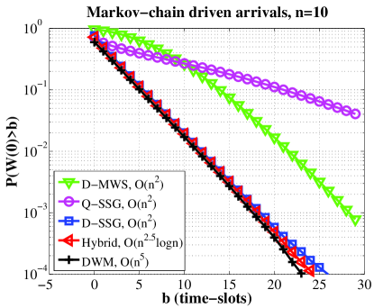
The results are summarized in Fig. 2, where the complexity of each policy is also labeled. In order to compare the rate-function as defined in Eq. (2), we plot the probability over the number of channels or users, i.e., , for a fixed value of threshold . The negative of the slopes of the curves can be viewed as the rate-function for each policy. In Fig. 2, we report the results only for , and the results are similar for other values of threshold . From Fig. 2, we observe that D-SSG has a similar delay performance to that of DWM and Hybrid, which are both known to be rate-function delay-optimal. This not only supports our theoretical results that D-SSG guarantees a near-optimal rate-function, but also implies that D-SSG empirically performs very well while enjoying a lower complexity. Further, we observe that D-SSG consistently outperforms its queue-length-based counterpart, Q-SSG, despite the fact that in [9], it has been shown through simulations that Q-SSG empirically achieves near-optimal queue-length performance. This provides a further evidence that good queue-length performance does not necessarily translate into good delay performance. The results also show that D-MWS yields a zero rate-function, as expected.
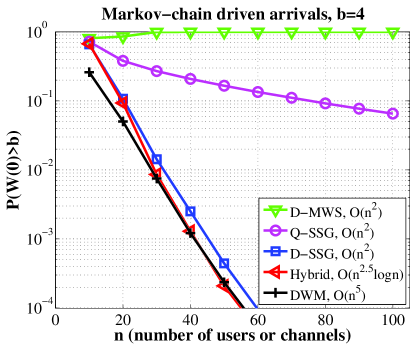
We also plot the probability for delay threshold as in [5, 9, 10, 12, 13, 15] to investigate the performance of different policies for fixed . In Fig. 3, we report the results for , and the results are similar for other values of . From Fig. 3, we observe that D-SSG consistently performs closely to DWM and Hybrid for almost all values of that we consider. We also observe that D-SSG consistently outperforms its queue-length-based counterpart, Q-SSG.
In addition, we compute the average time required for the operations of each policy within one scheduling cycle, when . Running simulations in a PC with Intel Core i7-2600 3.4GHz CPU and 8GB memory, D-SSG requires roughly 0.3 millisecond to finish all of the required operations within one scheduling cycle (which, for example, is 1 millisecond in LTE systems), while the two-stage Hybrid policy needs 7-10 times more. This, along with the above simulation results, implies that in practice D-SSG is more suitable for actual implementations than the hybrid policies, although D-SSG does not guarantee rate-function delay optimality.
Further, we evaluate scheduling performance of different policies in more realistic scenarios, where users are heterogeneous and channels are correlated over time. Specifically, we consider channels that can be modeled as a two-state Markov chain, where the channel is “ON” when the Markov chain is in state 1, and is “OFF” when it is in state 2. We assume that there are two classes of users: users with an odd index are called near-users, and users with an even index are called far-users. Different classes of users see different channel conditions: near-users see better channel condition, and far-users see worse channel condition. We assume that the transition probability matrices of channels for near-users and far-users are and , respectively. The arrival processes are assumed to be the same as in the previous case.
The results are summarized in Fig. 4. We observe similar results as in the previous case with homogeneous users and i.i.d. channels in time. In particular, D-SSG exhibits a rate-function that is similar to that of DWM and Hybrid, although its delay performance is slightly worse. Note that in this scenario, a rate-function delay-optimal policy is not known yet. Hence, for future work, it would be interesting to understand how to design rate-function delay-optimal or near-optimal policies in general scenarios.
VI Conclusion
In this paper, we developed a practical and low-complexity greedy scheduling policy (D-SSG) that not only achieves throughput optimality, but also guarantees a near-optimal delay rate-function, for multi-channel wireless networks. Our studies reveal that throughput optimality is relatively easier to achieve in such multi-channel systems, while there exists an explicit trade-off between complexity and delay performance. If one can bear a minimal drop in the delay performance, lower-complexity scheduling policies can be exploited.
The analytical results in this paper are derived for the i.i.d. ON-OFF channel model with unit channel capacity. An interesting direction for future work is to study general multi-rate channels that can be correlated over time. We note that this problem will become much more challenging. For example, even for an i.i.d. 0- channel model with channel capacity , it is still unclear whether there exists a scheduling policy that can guarantee both optimal throughput and optimal/near-optimal asymptotic delay performance. Another direction for future work is to consider heterogeneous users with different arrival processes and different delay requirements. In these more general scenarios, it may be worth exploring how to find efficient schedulers that can guarantee a nontrivial lower bound of the optimal rate-function, if it turns out to be too difficult to achieve or prove the optimal asymptotic delay performance itself. Nonetheless, we believe that the results derived in this paper will provide useful insights for designing high-performance scheduling policies for more general scenarios.
Appendix A Proof of Theorem 1
We consider event and a sequence of events implying the occurrence of event .
Event : Suppose that there is a packet that arrives to the network in time-slot . Without loss of generality, we assume that the packet arrives to queue . Further, suppose that is disconnected from all the servers in all the time-slots from to .
Then, at the beginning of time-slot 0, this packet is still in the network and has a delay of . This implies . Note that the probability that event occurs can be computed as
Hence, we have
and thus
Event : Consider any fixed . Fix any , and choose such that . Suppose that from time-slot to , the total number of packet arrivals to the system is greater than , and let denote the probability that this event occurs. Then, from the definitions of and , we know
Clearly, the total number of packets that are served in any time-slot is no greater than . Hence, at the end of time-slot , there are at least packets remaining in the system. Moreover, at the end of time-slot , the system contains at least one packet that arrived before time-slot . Without loss of generality, we assume that this packet is in . Now, assume that is disconnected from all the servers in the next time-slots, i.e., from time-slot to . This occurs with probability , independently of all the past history. Hence, at the beginning of time-slot 0, there is still a packet that arrived before time-slot . Hence, we have in this case. This implies . Note that the probability that event occurs can be computed as
Hence, we have
and thus
Since the above inequality holds for any and all , by letting tend to 0 and taking the minimum over all , we have
Considering both event and events , we have
Appendix B Strictly Positive Rate-function
Consider i.i.d. 0- arrivals: in each time-slot, there are packet arrivals with probability , and no arrivals otherwise. Clearly, the mean arrival rate must be smaller than 1, otherwise the system is not stabilizable and thus the rate-function of the delay-violation probability becomes zero under any scheduling policy. Hence, we want to show that our derived upper bound is strictly positive in the case of i.i.d. 0- arrivals with mean arrival rate .
Recall that , where , , and . It is easy to see that and for all . Hence, in order to show it suffices to show that . Also, note that is a non-decreasing function of , and thus is also non-decreasing. Therefore, it suffices to show . Let denote the number of queues that have arrivals in time-slot , and let . Also, let . Then, we have
where the last inequality is from the Chernoff bound, and , is the Kullback-Leibler divergence. Hence, , and . This completes the proof.
Appendix C Delay-based Queue-Side-Greedy (D-QSG) And Sample-Path Equivalence
Delay-based Queue-Side-Greedy (D-QSG) policy, in an iterative manner too, schedules the oldest packets in the system one-by-one whenever possible. In this sense, D-QSG can be viewed as an intuitive approximation of the Oldest Packet First (OPF) policies333A scheduling policy is said to be an OPF policy if in any time-slot, policy can serve the oldest packets in that time-slot for the largest possible value of . [15] that have been shown to be rate-function delay-optimal. We later prove an important sample-path equivalence result (Lemma 3) that will be used in proving Lemma 1 and thus the main result of this paper (Theorem 3).
We start by presenting some additional notations. In the D-QSG policy, there are at most rounds in each time-slot . By slightly abusing the notations, we let , and denote the length of queue , the delay of the -th packet of , and the HOL delay of after the -th round in time-slot under D-QSG, respectively. Let denote the set of indices of the available servers at the beginning of the -th round, and let denote the set of queues that have the largest HOL delay among all the queues that are connected to at least one server in at the beginning of the -th round, i.e., . Also, let be the index of the queue that is served in the -th round of time-slot , and let be the index of the server that serves in that round. We then specify the operations of D-QSG as follows.
Delay-based Queue-Side-Greedy (D-QSG) policy: In each time-slot ,
-
1.
Initialize and .
-
2.
In the -th round, allocate server to , where
That is, in the -th round, we consider the queues that have the largest HOL delay among those that have at least one available server connected (i.e., the queues in set ), and break ties by picking the queue with the smallest index (i.e., ). We then choose an available server that is connected to queue , and break ties by picking the server with the smallest index (i.e., server ), to serve . At the end of the -th round, update the length of to account for service, i.e., set and for all . Also, update the HOL delay of , by setting if , and otherwise, and setting for all .
-
3.
Stop if equals . Otherwise, increase by 1, set , and repeat step 2.
Remark: Note that D-QSG is only used for assisting the rate-function delay analysis of D-SSG and may not be suitable for practical implementation due to its complexity. This is because there are at most rounds, and in each round, it takes time to find a queue that has at least one connected and available server (which takes time to check for all queues) and that has the largest HOL delay (which takes time to compare).
The following lemma states the sample-path equivalence property between D-QSG and D-SSG under the tie-breaking rules specified in this paper.
Lemma 3
For the same sample path, i.e., same realizations of arrivals and channel connectivity, D-QSG and D-SSG pick the same schedule in every time-slot.
Proof:
We prove Lemma 3 by induction. It suffices to prove that for any given system, i.e., for any given set of packets after arrivals and for any channel realizations, both D-SSG and D-QSG pick the same schedule. Suppose that there are packets in the system. Let denote the -th oldest packet in the system. We want to show that packet is either served by the same server under both D-SSG and D-QSG, or is not served by any server under both D-SSG and D-QSG. We denote the set of the oldest packets by , and denote the set of the first servers by . Let denote the server allocated to serve the -th oldest packet under D-QSG. We prove it by induction method.
Base case: Consider packet , i.e., the oldest packet, and consider two cases: under D-QSG, 1) packet is served by ; 2) packet is not served by any server.
In Case 1), we want to show that packet is also served by the same server under D-SSG. Note that packet is the oldest packet in the system and is the first packet to be considered under D-QSG. Since it is served by , from the tie-breaking rule of D-QSG, we know that the queue that contains packet is disconnected from all the servers in set except server . Now, we consider the server allocation under D-SSG, which allocates servers one-by-one in an increasing order of the server index. Since all the servers in set except for server are disconnected from the queue containing packet , these servers cannot be allocated to packet in the first rounds under D-SSG. While in the -th round, D-SSG must allocate server to packet , since the queue that contains packet is the queue that has the largest HOL among the queues that are connected to server .
In Case 2), packet is the first packet to be considered under D-QSG, but is not served by any server. This implies that no servers are connected to the queue that contains packet . Hence, packet cannot be served under D-SSG either.
Combining the above two cases, we prove the base case.
Induction step: Consider an integer . Suppose that every packet in set is either served by the same server under both D-QSG and D-SSG, or is not served by any server under both D-QSG and D-SSG. We want to show that this also holds for every packet in set . Clearly, it suffices to consider only packet (i.e., the -th oldest packet in the system), as the other packets all satisfy the condition from the induction hypothesis. We next consider two cases: under D-QSG, 1) packet is scheduled by a server under D-QSG; 2) is not served by any server.
In Case 1), suppose that packet is served by server under D-QSG. We want to show that packet is also served by server under D-SSG. We first show that under D-SSG, packet cannot be served in the first rounds. Note that under D-QSG, packet is served by server . This implies that any server in set is either disconnected from the queue that contains packet or has already been allocated to packets in set under D-QSG. This, along with the induction hypothesis, further implies that under D-SSG, in the first rounds, the servers under consideration are either disconnected from the queue that contains packet or allocated to packets in set . Hence, packet cannot be scheduled in the first rounds under D-SSG. Next, we want to show that packet must be served by server in the -th round under D-SSG. Let denote the set of packets among the oldest packets that are not served under both D-QSG and D-SSG. Then, all the queues that contain packets in set must be disconnected from server , otherwise some packet should be served by server under D-QSG. On the other hand, the induction hypothesis implies that any packet must be served by some server , under D-SSG, where . Hence, D-SSG does not allocate server to any packet in set . Therefore, in the -th round, D-SSG must allocate server to packet , since the queue that contains packet has the largest HOL delay among the queues that are connected to server .
In Case 2), packet is not served by any server under D-QSG. This implies that the queue that contains packet is disconnected from all the servers in set , i.e., the set of available servers when considering packet . On the other hand, the induction hypothesis implies that under D-SSG, all the servers in set are also allocated to packets in set . Hence, packet cannot be served by any server under D-SSG either.
Combining the above two cases, we prove the induction step. This completes the proof. ∎
Note that under D-SSG, in each round, when a server has multiple connected queues that have the largest HOL delay, we break ties by picking the queue with the smallest index. Presumably, one can take other arbitrary tie-breaking rules. However, it turns out to be much more difficult to directly analyze the rate-function performance for a greedy policy from the server side (like D-SSG) without using the above equivalence property. For example, as we mentioned earlier, the authors of [9, 10] were only able to prove a positive (queue-length) rate-function for Q-SSG in more restricted scenarios. Hence, our choice of the above simple tie-breaking rule is in fact quite important for proving the above sample-path equivalence result, which in turn plays a critical role in proving a key property of D-SSG (Lemma 1) and thus near-optimal rate-function of D-SSG (Theorem 3). Nevertheless, we would expect that one can choose arbitrary tie-breaking rules for D-SSG in practice.
Appendix D Proof of Lemma 1
Lemma 4
Consider a set of packets. Consider any function , which is strictly increasing with . The D-SSG policy is applied to schedule these packets. Then, there exists a finite integer such that for all , with probability no smaller than , D-SSG schedules all the oldest packets among the packets.
Proof:
Since Lemma 4 is focused on the oldest packets in the set, it is easier to consider the D-QSG policy instead, which in an iterative manner schedules the oldest packets first. Due to the sample-path equivalence between D-SSG and D-QSG (Lemma 3), it is sufficient to prove that the result of Lemma 4 holds for D-QSG.
Suppose that the oldest packets among the packets are from different queues, where . It is easy to see that if each of the queues is connected to no less than servers, then all of these oldest packets will be served. Specifically, because D-QSG gives a higher priority to an older packet, the above condition guarantees that when D-QSG schedules any of the oldest packets, there will always be at least one available server that is connected to the queue containing this packet.
Now, consider any queue . We want to compute the probability that is connected to no less than servers. We first compute the probability that is connected to less than servers:
Next, choose such that and for all . Such an exists because and , hence, we have and thus for large enough ; and similarly, because and , hence, we have and thus for large enough . Then, the probability that each of the queues is connected to no less than servers is:
for all , where (a) is from our choice of and the fact that , (b) is from our choice of and Bernoulli’s inequality (i.e., for every real number and every integer ), and (c) is from our choice of . This completes the proof. ∎
Lemma 5
Consider a set of packets satisfying that no more than packets are from the same queue, where is any integer constant independent of . The D-SSG policy is applied to schedule these packets. Then, there exists a finite integer such that for all , with probability no smaller than , D-SSG schedules at least packets among the packets.
Proof:
Consider the D-SSG policy. We first compute the probability that some packets are not scheduled by D-SSG, which is equivalent to the event that some servers are not allocated to any packet by D-SSG.
Consider any arbitrary set of servers , where if . Clearly, we have for all . Consider the -th server . Then, the number of remaining packets is at least at the beginning of the -th round. Since no more than packets are from the same queue, there are at least queues that are non-empty at the beginning of the -th round. Then, the probability that server is not allocated to any packet is no greater than . Hence,
Since , there exists an such that for all . Such an exists because and , hence, and thus for large enough . Then, we can compute the probability that some servers are not allocated as
for all , where the last inequality is due to our choice of .
Therefore, we have
for all . ∎
Appendix E Proof of Theorem 4
The proof follows a similar argument for the proof of Theorem 2 in [13].
We start by defining . Consider any fixed , and define . Then, we have .
We then choose the value of parameter for G-FBS based on the statistics of the arrival process. We fix and . Then, from Assumption 3, there exists a positive function such that for all and , we have
for any integer . We then choose
The reason for choosing the above value of will become clear later on. Recall from Assumption 2 that is the maximum number of packets that can arrive to a queue in any time-slot . Then, is the maximum number of packets that can arrive to a queue during an interval of time-slots, and is thus the maximum number of packets from the same queue in a frame. This also implies that in the S-frame, no more than packets are from the same queue.
Next, we define the following notions associated with the G-FBS policy. Let denote the number of unserved frames in time-slot , and let denote the remaining available space (where the unit is packet) in the end-of-line frame at the end of time-slot . Also, let denote the indicator function of whether a success occurs in time-slot . That is, if there is a success, and otherwise. Recall that . Then, we can write a recursive equation for :
| (4) | ||||
| (5) |
Let denote the number of packets in the L-frame at the beginning of time-slot , and let denote the number of packets in the HOL frame at the beginning of time-slot . Then, at the beginning of time-slot , the number of packets in the S-frame is equal to . Let denote the number of packets served from the S-frame if a success occurs in time-slot . Then, we have the following recursive equation for :
Also, we let
denote the the total number of successes in the interval from time-slot to when the S-frame is non-empty (i.e., the number of unserved frames is greater than zero or the L-frame is non-empty).
Note that the arriving time of a frame is the time when its first packet arrives. Let denote the available space in the end-of-line frame at the end of time-slot . Then, we let denote the number of new frames that arrive from time-slot to . When , we use to denote for notational convenience.
Let be the last time before , when the number of unserved frames is equal to zero. Then, given that , where , the number of unserved frames never becomes zero during interval . Let denote the indicator function of whether at time-slot 0 the L-frame contains a packet that arrives before time-slot , i.e., if at time-slot 0 the L-frame contains a packet that arrives before time-slot , and , otherwise. Let denote the event that the number of frames that arrive during interval is greater than the total number of successes during interval when the S-frame is non-empty, i.e.,
Let denote the event that the number of frames that arrive during interval is equal to the total number of successes during interval when the S-frame is non-empty, and at time-slot the L-frame contains a packet that arrives before time-slot , i.e.,
Letting , we have
| (6) |
By taking the union over all possible values of and applying the union bound, we have
| (7) |
We divide the proof into two parts. In Part 1, we show that there exist a constant and a finite such that for all , we have
where is a function satisfying that and . And in Part 2, we show that there exists a finite such that for all , we have
Finally, combining both Parts, we have
for all . By letting tend to 0, and taking logarithm and limit as goes to infinity, we obtain , and thus the desired results.
We next present Lemma 6 that will be used in the proof.
Lemma 6
Consider the G-FBS policy. Let be an arrival process. Consider the interval , and recall that is the available space in the end-of-line frame at the end of time-slot . Suppose the following two conditions are satisfied:
-
1.
The number of unserved frames never becomes zero during interval , i.e., for all .
-
2.
For any consecutive time-slots in the interval, the cumulative arrivals are greater than or equal to , i.e., , for any .
Then the following holds,
Remarks: The result of the above lemma implies that every frame that arrives in interval (except for the last frame) has exactly packets. The proof follows an inductive argument for the proof of Lemma 9 in [13], and is thus omitted.
Part 1: Consider any . Let be the set of sample paths in which and occurs, let be the set of sample paths in which , and let denote the set of sample paths in which there are at least packet arrivals to the system during every consecutive time-slots in the interval of . Let be such that for all .
First, we want to show that for all , we have
| (11) |
In the following, we will show that , and then it is easy to see that .
For every sample path in set , is the last time before , when the number of unserved frames is equal to zero. Then, the number of unserved frames never becomes empty during interval , i.e.,
| (12) |
Also, there are at least packet arrivals to the system during every consecutive time-slots in the interval of . The above implies that the conditions of Lemma 6 hold, and hence,
| (13) |
Moreover, we have or for all . Otherwise, there must exist one time-slot such that and , which implies and thus contradicts with (6). This, along with (12), implies
| (14) |
Hence, for any sample path in set , we have . Let denote the number of packets in the -th frame that arrives in the interval . We want to show that for any sample path in the set , we have
| (15) |
Now, recall that for every sample path in set , there are two cases: either or occurs. We consider these two cases separately.
Case 1) Suppose occurs, i.e., . Then, from (13) and (14), we have . Eq. (13) also implies that all the frames that arrive in the interval , except the last frame, are fully filled (with packets). Since the -th frame is not the last frame, we have .
Case 2) Suppose occurs, i.e., and . Then, from (13) and (14), we have . This implies that the -th frame is the last frame. Now, suppose that . Then, the last success in the interval of would have completely cleared the packets as they are among the oldest packets. This implies , which contradicts with the assumption that occurs. Therefore, we must have .
Combining both cases, we show that (15) holds for any sample path in set .
Recall that for any sample path in set of , all the frames that arrive in the interval of , except the last frame, are fully filled (with packets), and that . Hence, we have
for all , where the last inequality is from (15), our choice of such that for all , and . Hence, we have . This implies for all , and thus (11) holds. Therefore,
Along with the choice of (as chosen earlier), we can show that there exist and such that for all ,
| (16) |
Here, we do not duplicate the detailed proof for (16), and refer the interested readers to [13] for details.
Next, we calculate the probability that event occurs. Specifically, we want to show that there exists a finite such that for all and for all , we have
Recall that and . Hence, for any fixed , there exists a finite such that for all , we have
| (17) |
We next calculate an upper bound on the probability that during interval , there are exactly successes, for some . Recall from Lemma 1 that for all , the probability of a success in each time-slot is no smaller than . Hence, we have
| (18) |
It is easy to observe that the right hand side is a monotonically increasing function in .
We choose such that for all , and choose . Using the results from (17) and (18), we have that for all ,
where (a) is from the monotonicity of the right hand side of (18), (b) is from (17) and (18), (c) is from changing variable by setting , and (d) is from our choice of .
Summing over to , we have
for all .
Part 2: We want to show that there exists a finite such that for all , we have
As in the proof for Theorem 2 of [13], for any fixed real number , we consider the arrival process , by adding extra dummy arrivals to the original arrival process . The resulting arrival process is simple, and has the following property:
Hence, if we can find an upper bound on , by our construction, then it is also an upper bound on .
Consider any . Let be the set of time-slots in the interval from to when . Given , from Lemma 6, we have that,
From Assumption 3 on the arrival process we know that for large enough and , can be made less than an arbitrarily small fraction of . Further, we can show that for and , we have . This is derived by substituting the values of and in the equation above,
Then, it follows that
| (19) |
for all and , where the last inequality is from Assumption 3 and (9).
We now state a lemma that will be used in the proof.
Lemma 7
Let be a sequence of binary random variables satisfying
where is a polynomial in of finite degree. Let be such that for all . Then, for any real number , we have
for all .
Proof:
The proof follows immediately from Lemma 1 of [13]. ∎
Moreover, we know from Lemma 1 that for each , with probability less than for all . Choose such that for all . Hence, choosing and using Lemma 7, we have
| (20) |
for all and .
Then, summing over all , we have that for all ,
where (a) is from our choice of , and (b) is from (8).
Combining both parts, the result of the theorem then follows.
Appendix F Proof of Lemma 2
Consider two queueing systems, and , both of which have the same arrival and channel realizations. We assume that adopts the D-SSG policy and adopts the G-FBS policy (with any value of ). We define the weight of a packet in time-slot as its delay, i.e., , where denotes the time when packet arrives to the system. Note that different packets (in the same queue or in different queues) may have the same delay. In order to make each packet in the system have a unique weight, we redefine the weight of a packet as , where denotes the index of the queue that contains packet and denotes that packet is the -th arrival to queue in time-slot . For two packets and , we say is older than if . Note that as in [12, 13], we use weight instead of for ease of analysis only.
Let denote the set of packets present in system at the end of time-slot , for . Then, it suffices to show that for all time-slot . We let denote the set of packets that arrive in time-slot . Let denote the set of packets that depart system at time , for . Hence, we have
We then proceed our proof by contradiction. Suppose that for some time-slot . Without loss of generality, we assume that time-slot is the first time such that occurs. Hence, there must exist a packet, say , such that but . Because is the first time when such an event occurs, packet must depart from system in time-slot while it is not served in system , i.e., and . Let denote the set of packets in with weight greater than , for . Clearly, we have for all , as by assumption. Let denote the set of servers that are chosen to serve packets in , for .
Now, consider time-slot . Given that packet is not served in system , we want to show that packet cannot be served in system either. From the hypothesis, we know that packet must be disconnected from any server in set , otherwise due to the operations of D-SSG, packet must be served by some server in set in system . Note that both systems have the same channel realizations. Hence, packet cannot be served by any server in set in system either. Next, we show that packet is not served by any server in set in system . Consider any server , which serves some packet in system (under D-SSG). Then, one of the following must occur in system (under G-FBS, which runs D-SSG over the oldest packets): either server also serves packet , or server is allocated to serve some packet with a larger weight than packet due to the operations of D-SSG and the fact that . This implies that packet is not served by any server in set in system . Therefore, packet is not served by any server in system . This leads to a contradiction that packet departs from system in time-slot , and thus completes the proof.
Appendix G Proof of Theorem 2
We first restate the definition of a class of throughput-optimal MWF policies, and then show that D-QSG is an MWF policy.
Recall that denotes the length of queue at the beginning of time-slot immediately after packet arrivals, denotes the delay of the -th packet of at the beginning of time-slot , denotes the delay of the HOL packet of at the beginning of time-slot , and denotes the connectivity between and in time-slot . Also, let denote the set of queues being connected to server in time-slot , i.e., , and let denote the subset of queues in that have the largest weight in time-slot , i.e., . Let be the index of the queue that is served by server in time-slot , under a scheduling policy . Policy is said to be an MWF policy if there exists a constant such that, in any time-slot and for all , queue satisfies that for all such that . It has been proven that any MWF policy is throughput-optimal [15].
Then, it remains to show that D-SSG is an MWF policy. Let . We want to show that in any time-slot and for all , D-SSG allocates server to serve queue , which satisfies that for all such that .
Consider any round in any time-slot , where server needs to be allocated. Also, consider any such that . Suppose that server is allocated to serve queue , then we have that , where the first inequality is because the HOL packet of queue at the beginning of time-slot must have a delay no smaller than the HOL packet of queue at the beginning of the -th round, the second inequality is due to the operations of D-SSG, and the last inequality is because the HOL packet of queue at the beginning of the -th round must have a delay no smaller than the -th packet in queue at the beginning of time-slot . This implies that the sufficient condition is satisfied under D-SSG. Therefore, D-SSG is an MWF policy and is thus throughput-optimal.
References
- [1] L. Ying, R. Srikant, A. Eryilmaz, and G. Dullerud, “A large deviations analysis of scheduling in wireless networks,” IEEE Transactions on Information Theory, vol. 52, no. 11, pp. 5088–5098, 2006.
- [2] A. Stolyar, “Large deviations of queues sharing a randomly time-varying server,” Queueing Systems, vol. 59, no. 1, pp. 1–35, 2008.
- [3] S. Shakkottai, “Effective capacity and QoS for wireless scheduling,” IEEE Transactions on Automatic Control, vol. 53, no. 3, pp. 749–761, 2008.
- [4] V. Venkataramanan and X. Lin, “On wireless scheduling algorithms for minimizing the queue-overflow probability,” IEEE/ACM Transactions on Networking, vol. 18, no. 3, pp. 788–801, 2010.
- [5] S. Bodas, S. Shakkottai, L. Ying, and R. Srikant, “Scheduling in multi-channel wireless networks: Rate function optimality in the small-buffer regime,” in ACM Proceedings of the eleventh international joint conference on Measurement and modeling of computer systems (SIGMETRICS), 2009, pp. 121–132.
- [6] C. Courcoubetis and R. Weber, “Buffer overflow asymptotics for a buffer handling many traffic sources,” Journal of Applied Probability, pp. 886–903, 1996.
- [7] S. Shakkottai and R. Srikant, “Many-sources delay asymptotics with applications to priority queues,” Queueing Systems, vol. 39, no. 2, pp. 183–200, 2001.
- [8] S. Kittipiyakul and T. Javidi, “Delay-optimal server allocation in multiqueue multiserver systems with time-varying connectivities,” IEEE Transactions on Information Theory, vol. 55, no. 5, pp. 2319–2333, 2009.
- [9] S. Bodas, S. Shakkottai, L. Ying, and R. Srikant, “Low-complexity scheduling algorithms for multi-channel downlink wireless networks,” in The IEEE International Conference on Computer Communications (INFOCOM). IEEE, 2010, pp. 1–9.
- [10] ——, “Scheduling for small delay in multi-rate multi-channel wireless networks,” in The IEEE International Conference on Computer Communications (INFOCOM). IEEE, 2011, pp. 1251–1259.
- [11] S. Bodas and T. Javidi, “Scheduling for multi-channel wireless networks: Small delay with polynomial complexity,” in 2011 International Symposium on Modeling and Optimization in Mobile, Ad Hoc and Wireless Networks (WiOpt). IEEE, 2011, pp. 78–85.
- [12] M. Sharma and X. Lin, “OFDM downlink scheduling for delay-optimality: Many-channel many-source asymptotics with general arrival processes,” in The IEEE Information Theory and Applications Workshop (ITA), 2011.
- [13] ——, “OFDM downlink scheduling for delay-optimality: Many-channel many-source asymptotics with general arrival processes,” Purdue University, Tech. Rep., 2011. [Online]. Available: https://engineering.purdue.edu/%7elinx/papers.html
- [14] B. Ji, C. Joo, and N. B. Shroff, “Delay-Based Back-Pressure Scheduling in Multihop Wireless Networks,” IEEE/ACM Transactions on Networking, vol. 21, no. 5, pp. 1539–1552, 2013.
- [15] B. Ji, G. R. Gupta, X. Lin, and N. B. Shroff, “Low-complexity scheduling policies for achieving throughput and asymptotic delay optimality in multi-channel wireless networks,” IEEE/ACM Transactions on Networking, 2013, accepted for publication.
- [16] A. Mekkittikul and N. McKeown, “A starvation-free algorithm for achieving 100% throughput in an input-queued switch,” in Proc. of the IEEE International Conference on Communication Networks (ICCCN), 1996.
- [17] M. Andrews, K. Kumaran, K. Ramanan, A. Stolyar, P. Whiting, and R. Vijayakumar, “Providing quality of service over a shared wireless link,” IEEE Communications magazine, vol. 39, no. 2, pp. 150–154, 2001.
- [18] S. Shakkottai and A. Stolyar, “Scheduling for multiple flows sharing a time-varying channel: The exponential rule,” Translations of the American Mathematical Society-Series 2, vol. 207, pp. 185–202, 2002.
- [19] M. Andrews, K. Kumaran, K. Ramanan, A. Stolyar, R. Vijayakumar, and P. Whiting, “Scheduling in a queuing system with asynchronously varying service rates,” Probability in the Engineering and Informational Sciences, vol. 18, pp. 191–217, 2004.
- [20] A. Eryilmaz, R. Srikant, and J. Perkins, “Stable scheduling policies for fading wireless channels,” IEEE/ACM Transactions on Networking, vol. 13, no. 2, pp. 411–424, 2005.
- [21] B. Sadiq and G. de Veciana, “Throughput optimality of delay-driven MaxWeight scheduler for a wireless system with flow dynamics,” in Proceedings of the 47th Annual Conference on Communication, Control and Computing (Allerton), 2009.
- [22] M. Neely, “Delay-based network utility maximization,” in The 29th IEEE International Conference on Computer Communications (INFOCOM), 2010.
- [23] M. Bramson, “Stability of queueing networks,” Probability Surveys, vol. 5, no. 1, pp. 169–345, 2008.
- [24] J. Dai, “On positive Harris recurrence of multiclass queueing networks: a unified approach via fluid limit models,” The Annals of Applied Probability, pp. 49–77, 1995.