Inferring Attitude in Online Social Networks Based On Quadratic Correlation

Abstract

The structure of an online social network in most cases cannot be described just by links between its members. We study online social networks, in which members may have certain attitude, positive or negative toward each other, and so the network consists of a mixture of both positive and negative relationships. Our goal is to predict the sign of a given relationship based on the evidences provided in the current snapshot of the network. More precisely, using machine learning techniques we develop a model that after being trained on a particular network predicts the sign of an unknown or hidden link. The model uses relationships and influences from peers as evidences for the guess, however, the set of peers used is not predefined but rather learned during the training process. We use quadratic correlation between peer members to train the predictor. The model is tested on popular online datasets such as Epinions, Slashdot, and Wikipedia. In many cases it shows almost perfect prediction accuracy. Moreover, our model can also be efficiently updated as the underlaying social network evolves.

Keywords: Signed Networks, positive link, negative link, machine learning, quadratic optimization

1 Introduction

Online social networks provide a convenient and ready to use model of relationships between individuals. Relationships representing a wide range of different social interactions in online communities are useful for understanding and analyzing individual attitude and behaviour as a part of a larger society.

While the bulk of research in the structure on social networks tries to analyze a network using the topology of links (relationships) in the network [23], relationships between members of a network are much richer, and this additional information can be used in many areas of social networks analysis. In this paper we consider signed social networks, which consist of a mixture of both positive and negative relationships. This type of networks has attracted attention of researchers in different fields [7, 12, 19]. Understanding the interplay of relationships of different signs in the online social network setting is crucial for the design and function of many social computing applications, where we concern about the attitude of their members, trust or distrust they feel, known similarities and dissimilarities. For example, recommending new connections to their users is a common task in many online social networks. Yet, without the understanding of the type of relationships, an enemy can be introduced to a user as a friend. This framework is also quite natural in recommender systems [4, 25] where we can exploit similarities as well as dissimilarities between users and products.

Over the last several years there has been a substantial amount of work done studying signed networks, see, e.g. [17, 8, 10, 6, 15]. Some of the studies focused on a specific online network, such as Epinions [10, 21], where users can express trust or distrust to others, a technology news site Slashdot [15, 16], whose users can declare others ‘friends’ or ‘foes’, and voting results for adminship of Wikipedia [6]. Others develop a general model that fits several different networks [8, 17]. We build upon these works and attempt to combine the best in the two approaches by designing a general model that nevertheless can be tuned up for specific networks.

Edge sign prediction

Following Guha et al. [10] and Kleinberg et al. [17], [19] we consider a signed network as a directed (or undirected) graph, every edge of which has a sign, either positive to indicate friendship, support, approval, or negative to indicate enmity, opposition, disagreement. The edge sign prediction problem, in which given a snapshot of the signed network, the goal is to predict the sign of a given link using the information provided in the snapshot. Thus, the edge sign problem is similar to the much studied link prediction problem [18, 13], only we need to predict the sign of a link rather than the link itself.

Several different approaches have been taken to tackle this problem. Kunegis et al. [5] studies the friends and foes on Slashdot using network characteristics such as clustering coefficient, centrality and PageRank; Guha et al. [10] used propagation algorithms based on exponentiating the adjacency matrix to study how trust and distrust propagate in Epinion. Later Kleinberg et al. [17] took a machine learning approach to identify features, such as local relationship patterns and degree of nodes, and their relative weight and build a general model to predict the sign of a given link. They would train their predictor on some dataset, to learn the weights of these features by logistic regression. Once trained, the model can be used on different networks. Clearly, one of the most important measures of an approach is the accuracy of prediction it provides. Remarkably, in many cases (where comparable) the network independent approach from [17] provides more accurate predictions than that of previous network specific studies. This shows certain potential of machine learning techniques. Interestingly, this study is also related to the status and balance theories from social psychology [7, 14], as they rely on configurations similar to the features exploited in [17].

In this paper we also take the machine learning approach, only instead of focusing on a particular network or building a general model across different networks, we build a model that is unique to each individual network, yet can be trained automatically on different networks. Such an approach intuitively should be capable of more accurate predictions than network independent methods, and it remain practically feasible.

Trusted peers and influence

The basic assumption of our model is that users’ attitude can be determined by the opinions of their peers in the network (compare to the balance and status theories [7, 14] from social psychology discussed in [17]). Intuitively speaking, peer opinions are guesses from peers on the sign of the link from a source node to a target node. Also, we assume that peer opinions are only partially known, some of them are hidden. We introduce three new components into the model: set of trusted peers, influence, and quadratic correlation technique.

When we try to count on peer opinions, not all such opinions are equally reliable, and we therefore choose a set of trusted peers whose opinions are important in determining the user’s action. The set of trusted peers is one of the features our algorithm learns during the training phase. Ideally, it would be good to have a set of trusted peers for each link in the network. However, considering the sparsity and the enormous size of the network, we cannot always afford to determine a set of trusted peers for every possible relationships. Instead, we find a set of trusted peers for each individual node. The optimal composition of such a set is not quite trivial, because even trusted peers may disagree, and sometimes it is beneficial to have trusted peers who disagree. Thus, to make reliable estimations on all relationships starting at the individual nodes, its set of trusted peers has to form a wide knowledge base on other nodes in the network.

While peer opinions provide very important information, this knowledge is sometimes incomplete. Relying solely on peer opinions implies that the attitude of a user would always agree with the attitude of a peer. However, in reality, there are often exceptions. What also matters is how this opinion correlates with the opinion of the user we are evaluating. To take this correlation into account we introduce another feature into the model, influence. Suppose the goal is to learn the sign of the link between user $A$ and user $B$, and $C$ is a peer of $A$. Then if $A$ tends to disagree with $C$, then positive attitude of $C$ towards $B$ should be taken as indication that $A$’s attitude towards $B$ is less likely to be positive. The opinion of $C$ is then considered to be the product of his attitude towards $B$ and his influence on $A$. Usually, influence is not given in the snapshot of the network. For example in the Wikipedia adminship dataset the explicit information is a collection of results of voting, while the correlation between the ways members vote is hidden and has to be learned together with other unknown parameters. We experimented with different ways of defining peer opinion, and found that using relationships and influences together to approximate peer opinions is more effective than using relationships along.

To learn the weights of features providing the best accuracy we have chosen to use the standard quadratic correlation technique from machine learning [11]. This method involves finding the optimum of a quadratic polynomial, and while being relatively computationally costly, tends to provide very good accuracy. Therefore to solve quadratic programs we resort to three approaches. Firstly, we used an available Max-SAT solver METSLib [2] based on the Tabu search heuristics. Secondly, we also attempted to find the exact optimal solution using the brute force approach. Third, we use off-the-shelf solver Cplex [1]. Clearly, in the latter two approaches it is not feasible to solve the quadratic program arising from a large network, therefore we also used a number of heuristics to split such a program, as described later. An interesting use of our approach is to apply the quantum annealing devise developed by D-Wave [20] to run our algorithm. This devise solves large instances of the Quadratic Unconstrained Binary Optimization problem (QUBO) with (supposedly) high accuracy and high speed. However, such experimentation is yet to be done because the device is currently unavailable for experimenting.

Comparison to other work

Similar to [17, 8] we also use a machine learning approach to build a prediction model based on local features. However, unlike their generalized features, such as the degree of nodes, and local relationship patterns, we use peer opinions from trusted peers which are personalized features. There are two main advantages for using personalized features. First of all, our model tolerates differences in individual personalities. Unlike existing approach, two nodes with the same local features can behave differently by selecting different sets of trusted peers. Yet the model of Kleinberg et al. [17] treats nodes with the same feature values as the same. Secondly, our model accommodates the dynamic nature of online social networks. Personalized features allow us to train a predictor separately for each individual node. As the network evolves over time, we only need to update individual predictors separately instead of rebuilding the whole model. Although our model does not generalize across different datasets, a new model can be easily trained for different datasets without changing the algorithm.

We build and test our model on three different datasets studied before, Epinions, Slashdot and Wikipedia. It is difficult, however, to compare our results against the results in other works such as [10, 5, 17, 8]. For example [10] and [17] use certain (different!) normalization techniques to eliminate the bias of the datasets above toward positive links. We therefore tried to test our model in all regimes used in the previous papers. The results shows similar or better prediction accuracy in almost all cases. When tested on unchanged (biased) datasets our model shows nearly perfect prediction. In spite of this, fair comparison is still problematic, because of the lack of data about other approaches. For example, even the experiment results show that our model has a better prediction accuracy than the model in  [8] statistically, we couldn’t simply conclude our model is better because they used some normalization technique on the dataset, and also, it was not specified which edge embeddedness threshold (widely used in [17]) was used for the experiment.

Also, we test the model on a different dataset, MovieLens [3], used to recommend users movies to rent. Experiments show that we achieve good prediction accuracy on this dataset as well.

2 Approach

We now describe our method. We start with the underlying model of a network, then proceed to the machine learning formulation of the edge sign prediction problem, and finally describe the method to solve the resulting quadratic optimization problem.

2.1 Underlying Model

We are given a snapshot of the current state of a network. A snapshot of a network is represented by a directed graph $G=(V,E)$, where nodes represent the members of the network and edges the known or explicit links (relationships). Some of the links are signed to indicate positive or negative relationships. Let $s_{a,b}$ denote the sign of the relationship from $a$ to $b$ in the network. It may take two different values, $\{-1,1\}$, indicating negative and positive relationships respectively. Note that nodes of $G$ may represent entities of different kinds. For example, a signed relationship can also indicate the like or dislike of a product from a user, or the vote from a voter to a candidate.

To estimate the sign $s_{a,b}$ of a relationship from $a$ to $b$, we collect peer opinions. By a peer we understand a node in the network that we use to estimate $s_{a,b}$. In different versions of the models a peer can be any node of the network, or any node linked to $a$. Peer opinion is an important unknown parameter of the model. It is an estimation on the type of the relationship from a peer based on its own knowledge. Let $p^{c}_{a,b}\in\{-1,0,1\}$ denote the peer opinion of peer $c$ on the sign $s_{a,b}$. When $p^{c}_{a,b}=1$ or $p^{c}_{a,b}=-1$, it indicates that the $c$ believes that $s_{a,b}=1$ or $s_{a,b}=-1$ respectively. When $p^{c}_{a,b}=0$ that means $c$ does not have enough knowledge to make a valid estimation.

Another assumption made in our model is that not every peer can make a reliable estimation. Therefore we divide all peers of a node into two categories, and count the opinions only of the peers from the first category, trusted peers. The problem of how to select a set of trusted peers and use their opinions for the estimation will be addressed later. Let $P_{a}$ denote the set of trusted peers of $a$. We estimate the sign $s_{a,b}$ of a relationship from $a$ to $b$ by collecting the opinions of peers $c\in P_{a}$. If the sum of the opinions is nonnegative, then we say $s_{a,b}$ should be $1$, otherwise, it should be $-1$. This can be expressed by a simple equation as,

$$s_{a,b}=sign(\sum_{c\in P_{a}}p^{c}_{a,b})$$ (1)

Notice that the set of trusted peers $P_{a}$ for each node $a$ is also an unknown parameter. Determining the set of nodes in the set of trusted peers is a nontrivial task. Observe, for example, that the prediction accuracy does not necessarily increase as we add nodes, even nodes of higher trust into the set. Since the estimation are made by collecting opinions from all peers in the set, a correct estimation from one peer can be canceled by the wrong estimation of another. Also, it is beneficial to select a set of peers with more diversity without compromising accuracy. As mentioned earlier, the set of trusted peers of a node $a$ is crucial for the estimation of all relationships starting from $a$. Hence, having a set of peers that make good individual estimation on relationships to different sets of target nodes rather than nodes that make good individual estimation for the same set of target nodes will likely improve the accuracy of prediction.

2.2 Machine learning approach

Our approach to selecting an optimal set of trusted peers is to consider the quadratic correlations between each pair of peers. The overall performance of a set of peers is determined by the sum of the individual performance of each of them together with the sum of their performance in pairs. The individual performance measures the accuracy of individual estimations, while the pairwise performance measures the degree of difference between the estimations of the pair of peers. We want to maximize the accuracy of each individual and the diversity of each pair at the same time.

The loss function

Our goal is to use the information in $G$ to build a predictor $S(x,y)$ that predicts the sign $s_{x,y}$ of an unknown relationship from $x$ to $y$ with high accuracy. At the same time, we would also determine the unknown parameters used in the model. Our goal can be expressed by the objective function below,

$$min_{S}\{\sum_{x,y}(S(x,y)-s_{x,y})^{2}\}.$$ (2)

Least square loss function is the standard loss function used in measuring the prediction error. Another important reason for us to pick the square loss function is that it helps to capture quadratic correlations between all pairs of nodes in $V$. The quadratic correlation becomes more clear when the term gets expanded later in the next section.

Function $S(x,y)$ is defined as the sign of the sum of peer opinions as follows. Let

$$F_{x}(y)=\sum_{z\in P_{x}}p^{z}_{x,y}$$ (3)

denote the sum of individual peer opinions. Then we set

$$S(x,y)=\left\{\begin{array}[]{l l}1&\quad\mbox{if $F_{x}(y)\geq 0$ }\\ -1&\quad\mbox{if $F_{x}(y)<0$}\\ \end{array}\right.$$ (4)

Since $P_{x}$ is unknown, we introduce a new variable $w_{z,x}\in\{0,1\}$ which indicates if a node $z\in V$ should be included into set $P_{x}$. Hence, we rewrite Equation (3) using the characteristic function $w_{z,x}$ as,

$$F_{x}(y)=\sum_{z\in V}w_{z,x}p^{z}_{x,y}$$ (5)

Quadratic optimization problem

We are now ready to set the machine learning problem. A training dataset (a subset of $G$) is given. Every entry of the training dataset is a known edge along with its sign. Let a training dataset be $D=\{(x_{i},y_{i},s_{x_{i},y_{i}})|i=1,...,M\}$. The goal is to minimize the objective function, finding the optimal weight vector $w=\{w_{x}|x\in V\}$, where $w_{x}=\{w_{z,x}|z\in V\}$. We use machine learning methods [11] to train the predictor $S(x,y)$ and learn an optimal weight vector such that the objective function (2) is minimized. Substituting $S(x,y)$ and $F_{x}(y)$ into the objective function (2) we obtain quadratic unconstrained binary optimization (QUBO) problem described by equation (6).

$$w^{opt}=argmin_{w}\left(\sum_{(x,y,s_{x,y})\in D}(\frac{1}{N}\sum_{z\in V}(w_{z,x}p^{z}_{x,y}-s_{x,y})^{2})\right)$$ (6)

We want to minimize the amount of error made by $S(x,y)$, yet at the same time, we could also want to avoid overfitting. So we introduce the second term which is the regularization function based on the $L0$-norm. It ensures that the size of $P_{x}$ is not too large. The parameter $\lambda$ controls the trade off between the accuracy of the prediction and the complexity of the set $P_{x}$. Thus, the final form of the objective function is as follows

$$w^{opt}=argmin_{w}\left(\sum_{(x,y,s_{x,y})\in D}\left(\frac{1}{N}\sum_{z\in V}(w_{z,x}p^{z}_{x,y}-s_{x,y})^{2}+\lambda|w|\right)\right)$$ (7)

Note that there will be more details on peer opinion terms $p^{z}_{x,y}$.

2.3 Peer opinion variants

As mentioned earlier, we are going to test our model using different peer opinion formulations. First, let $s^{\prime}_{x,y}$ be extension of $s_{x,y}$ to edges with unknown sign and also to pairs of nodes that are not edges defined by

$$s^{\prime}_{x,y}=\left\{\begin{array}[]{ll}s_{x,y}&\mbox{if $s_{x,y}$ exists},\\ 0,&\mbox{otherwise}.\end{array}\right.$$

Simple-adjacent

The simplest option, later referred to as Simple-adjacent, is, based on the given information, to formulate peer opinions using existing relationships from peers to the target node. In other words, in this case we set $p^{z}_{x,y}$ to be $s^{\prime}_{z,y}$.

However, we also understand that the relationship from a peer to the target node does not always agree with the relationship from the source node to the target node. Yet, peers whose attitudes always disagree with the sources node are as important as these whose attitudes agree with the source node. In order to take the advantage of these disagreements, we introduced a second parameter, influence, which can be either positive, negative, or neutral.

Standard-pq

The second and third options differ in who is considered as a peer. In the Standard-pq option the influences $r_{x,y}\in\{-1,0,1\}$ associated with each pair of vertices $x,y$ is an unknown parameter in the model. In a sense every pair of nodes is assumed to be linked, thus turning $G$ into a complete graph. A positive influence, $r_{x,y}=1$, indicates that the attitude of $x$ affects $y$ positively, while a negative influence, $r_{x,y}=-1$ indicates that the attitude of $x$ affects $y$ negatively. Then the we obtain the standard formulation,

$$p^{z}_{x,y}=s^{\prime}_{z,y}r_{z,x}$$ (8)

Since the standard formulation gives us the best result in experiments, we use it throughout our discussion. Using the standard formulation, we rewrite Equation (5) as

$$F_{x}(y)=\sum_{z\in V}w_{z,x}s^{\prime}_{z,y}r_{z,x}.$$ (9)

Standard-adjacent

Finally, in the Standard-adjacent option peers of $x$ are restricted to the neighbours of $x$.

$$F_{x}(y)=\sum_{z\in N(x)}w_{z,x}s^{\prime}_{z,y}r_{z,x}.$$

The rest is defined in the same way as for the Standard-pq option.

2.4 Simplifying the model

In our model, we are given a directed complete graph $G=(V,E)$. In Equation (9), both $w_{z,x}$ and $r_{z,x}$ are unknown parameters. Since $r_{z,x}\in\{-1,0,1\}$, we can reduce the number of unknown parameters by considering all possible values of $r_{z,x}$, and rewriting $F_{x}(y)$ as,

$$F_{x}(y)=\sum_{z\in V}w_{z,x}^{+}s^{\prime}_{z,y}-w_{z,x}^{-}s^{\prime}_{z,y}$$ (10)

where $w_{z,x}=w_{z,x}^{+}+w_{z,x}^{-}$ for $w_{z,x}^{+},w_{z,x}^{-}\in\{0,1\}$. If $w_{z,x}^{+}=1$, then $z\in P_{x}$ and $r_{z,x}=1$. Similarly, $w_{z,x}^{-}=1$ indicates that $z\in P_{x}$ and $r_{z,x}=-1$. When both $w_{z,x}^{-}=0$ and $w_{z,x}^{+}=0$, then $z\not\in P_{x}$. Although $r_{z,x}$ can take three possible values, there are only two terms in Equation (9) since when $r_{z,x}=0$, the term is also zero regardless of the value of $s^{\prime}_{z,y}$.

Now to minimize the objective function, we need to determine the optimal weight vector $w=\{w_{x}|x\in V\}$ where $w_{x}=\{w_{z,x}^{+},w_{z,x}^{-}|z\in V\}$ such that

$$w^{opt}=argmin_{w}\left(\sum_{(x,y,s_{x,y})\in D}\left(\frac{1}{N}\sum_{z\in V}(w_{z,x}^{+}-w_{z,x}^{-})s^{\prime}_{z,y}-s_{x,y}\right)^{2}+\lambda|w|\right)$$ (11)

To find the optimal solution of $w$, we need to solve a QUBO of $2n^{2}$ variables which is very difficult since there are usually millions of nodes in a social network. Luckily, from the definition, we know $w_{x}$ and $w_{y}$ are independent for different nodes $x$ and $y$. Instead of solving for $w^{opt}$ directly, we can solve $w_{x}^{opt}$ for each $x\in V$ separately, and then combine their values to get $w^{opt}=\{w_{x}^{opt}|x\in V\}$.

$$w_{x}^{opt} = argmin_{w_{x}}\left(\sum_{(x,y,s_{x,y})\in D}\left(\frac{1}{N}\sum_{z\in V}(w_{z,x}^{+}-w_{z,x}^{-})s^{\prime}_{z,y}-s_{x,y}\right)^{2}+\lambda|w_{x}|\right)$$

$$= argmin_{w_{x}}\left(\frac{1}{N^{2}}\sum_{v\in V}\sum_{u\in V}(w_{v,x}^{+}-w_{v,x}^{-})(w_{u,x}^{+}-w_{u,x}^{-})\left(\sum_{(x,y,s_{x,y})\in D}s^{\prime}_{v,y}s^{\prime}_{u,y}\right)\right.$$

$$\ \ +\sum_{z\in V}(w_{z,x}^{+}-w_{z,x}^{-})\left(\lambda-\frac{2}{N}\sum_{(x,y,s_{x,y})\in D}s^{\prime}_{z,y}s^{\prime}_{x,y}\right)\Bigg{)}$$

Now, instead of solving a QUBO of size $2n^{2}$, we could solve $n$ QUBOs of size $2n$ separately. It can be solved approximately by a Max-SAT solver

If we use a different approach (similar to [22]), the problem should be further simplified, as it is still challenging to solve each of these size $2n$ QUBOs exactly.

Breaking down the problem

In order to find a good approximation of the optimal solution to the QUBO defined by Equation (2.4), we could break it down to much smaller QUBOs. Given a subset $U\subset V$, let $w_{x,U}=\{w_{z,x}^{+},w_{z,x}^{-}|z\in U\}$, and define a restricted optimization problem as follows

$$w_{x,U}^{opt}=argmin_{w_{x,U}}\left(\sum_{(x,y,s_{x,y})\in D}\left(\frac{1}{N}\sum_{z\in U}(w_{z,x}^{+}-w_{z,x}^{-})s_{z,y}-s_{x,y}\right)^{2}+\lambda|w_{x,u}|\right)$$

By the definition when $U=V$, Equation (2.4) is exactly the same as  (2.4), However, if we allow $U$ to be a subset of much smaller size, then the QUBO we need to solve is a much smaller size as well. By decreasing the size of $U$, we are trading the solution accuracy with the computational efficiency. Our intuition is to arrange nodes in $V$ according to some order, and then, we break $V$ into several smaller subsets. By solving Equation (2.4) on each of the subsets $U$, and combining their solutions, we can get a good approximation to the optimal solution of Equation (2.4). In the next section, we are going to explain the method used to approximate the optimal value of $w_{x}$ in detail.

2.5 Method

The optimization problem defined by Equation (2.4) is a quadratic unconstrained binary optimization problem which is NP-hard in general. To solve the optimization problem, we use two approaches. First, we solve problems of the form (2.4) separately using an open source Max-SAT solver METSLib based on the Tabu search heuristics. Second, we apply a similar method as described in [22] to reduce the size of the problem dramatically.

Under the second approach we break the original problem into even smaller subproblems and we obtain an approximate solution by combining the solutions of each subproblems. Algorithm 1 describes the method we used to solve each subproblems. Algorithm 2 uses Algorithm 1 as a subroutine and explains how the problem is broken down into subproblems and also how to combine the solutions of subproblems to obtain an approximate solution. During the training process, we need to use graph $G$ and dataset $D$. Moreover, $D$ is randomly split into two parts, training dataset $TD$ and validation dataset $VD$. We use $TD$ to train the predictor $S(x,y)$ and we use $VD$ to validate the predictors obtained at each step to select the optimal one.

According to Algorithm 2, we split $V$ into smaller subsets in two steps. First of all, for each $a\in V$ and for each $v\in V$, we compute the individual prediction error of $v$ for $a$ on the dataset $TD$ as follows: For each data point $(a,u,s_{a,u})\in TD$, we count $e_{v_{-}}$, the number of instances $p^{v}_{a,u}\neq s_{a,u}$ when $r_{v,a}=-1$, and $e_{v_{+}}$, the number of instances $p^{v}_{a,u}\neq s_{a,u}$ when $r_{v,a}=1$ separately. Note that since $p^{v}_{a,u}=r_{v,a}s^{\prime}_{v,u}$, we can compute this number; and that if $u$ is not a neighbour of $v$ then it contributes to both $e_{v_{-}}$ and $e_{v_{+}}$. Then, we replace $v$ by $v_{+}$ and $v_{-}$ with individual prediction error, $e_{v_{+}}$ and $e_{v_{-}}$ respectively. Second, using their individual prediction errors, we can sort the nodes in $V$ in increasing order of the error. The subset $U$ is iteratively selected by picking the first $d$ nodes in the list that are not yet considered. The value of $d$ is an important parameter of the algorithm and is selected manually at the beginning of the algorithm. If $d=n$, then we are solving the problem defined by Equation (2.4). The sorting and selecting processes not only reduce the amount of computation, but also allow us to consider the relevant nodes first.

Once the subset $U$ is selected, we use Algorithm (1) to solve the subproblem defined by Equation 2.4. The algorithm determines the optimal value of $w_{x,U}$ and the set $P_{x}\in U$ which minimize the amount of prediction errors made by $S(x,y)$. It repeatedly solves the QUBO for different $\lambda\in[\lambda_{min},\lambda_{max}]$ (in our experiments we use $\lambda_{min}=0.1$ and $\lambda_{max}=0.35$). $\lambda_{min}$ and $\lambda_{max}$ bound the possible range for $\lambda$, and the best value of $\lambda$ is selected using cross-validation on dataset $VD$. The set $P_{x}$ together with the weight $w_{x,U}$ which produces the lowest prediction errors on $VD$ is selected as the optimal solution. Notice, when the size of $U$ is small, say $d=10$, we can solve it exactly using brute-force method. When its size is larger, we use some heuristic methods such as the quadratic optimization solver Cplex [1] to approximate the solution.

The optimal solution determined by Algorithm 1 on subset $U$ is used to extend the optimal solution for $w_{x}$ by Algorithm 2. To extend the solution, we use a greedy approach similar to AdaBoost [9]. We would extend the partial solution, as long as extending it by the optimal solution on $U$ lowers the prediction error on the validation set $VD$.

Algorithm 1 Set the parameter for a subset

0:  training dataset: $TD$, validation dataset: $VD$, a subset of nodes: $U$

0:  values of $w$ and $Z\subset U$

  $Z=\emptyset$

  $e_{min}$ = $|TD|$

  for $\lambda=\lambda_{min}$ to $\lambda_{max}$ do

     $Z_{current}=\emptyset$

     solve the optimization $w^{opt}=argmin_{w}(\sum_{i=1}^{M}(\frac{1}{N}\sum_{z\in U}(w_{z}^{+}-w_{z}^{-})s_{z,y}-s_{x,y})^{2}+\lambda|w|)$

     if  $w_{z}$ == 1 then

        $Z_{current}$ = $Z_{current}\cup z$

     end if

     Measure the validation error $e_{val}$ on $vd$ using $Z_{current}$

     if  $e_{val}<e_{min}$ then

        $Z_{final}$ =$Z$

        $e_{min}$ = $e_{val}$

     end if

  end for

Algorithm 2 solve the optimization problem

0:  training dataset: $TD$, validation dataset: $VD$, The size of the subset: $d$

0:  values of $w_{z}$ for $z\in V$, and the set of trusted peers $Z$

  $e_{old}$ = $|TD|$

  $e_{new}$ =$|TD|$-1

  $Z=\emptyset$

  $Z_{current}=\emptyset$

  sort nodes of $V$ by their individual prediction errors in increasing order

  $U$ = the first $d$ nodes in $V$

  while $e_{old}>e_{new}$ do

     $Z$ = $Z_{current}\cup Z$

     $w_{z}$, $Z_{current}$ = Algorithm 1($td$, $vd$, $U$)

     $e_{old}$=$e_{new}$

     Measure the validation error $e_{new}$ on $vd$ using $Z$

     update $U$ with the next $d$ nodes in $V$

  end while

3 Datasets

We use three datasets borrowed from [17] and a movie rental dataset Movielens that we consider separately. In order to make comparison possible the datasets are unchanged rather than updated to their current status. The dataset statistics is therefore also from [17] (see Table 1).

Epinions

This is a web site dedicated to reviews on a variety of topics including product reviews, celebrities, etc. The feature of Epinion interesting to us is that users can express trust or distrust to each other, making it a signed social network. The dataset contains 119,217 nodes, 841,200 edges, 85% of which are positive and 15% are negative.

Slashdot

Slashdot is another web site for technology news where users are allowed to leave comments. It also has an additional Zoo feature that allows users tag each other as ‘friends’ and ‘foes’. This dataset contains 82,144 nodes, 549,202 edges of which 77.4% are positive and 22.6% are negative.

Wikipedia

This dataset contains Wikipedia users and the results of voting among them for adminship. Every link represents a vote of one user for or against another. A link is positive if the user voted for another and negative otherwise. It contains 7,118 nodes representing users who casted a vote or been voted for, 103,747 edges, of which 78.7% are positive and 21.2% are negative.

Table 1: Basic statistics on the datasets

Dataset	Epinions	Slashdot	Wikipedia
Nodes	119217	82144	7118
Edges	841200	549202	103747
+1 edges	85.0%	77.4%	78.7%
-1 edges	15.0%	22.6%	21.2%

4 Experiment

4.1 Parameters of datasets

In our experiment, we split each dataset into two parts. We randomly pick one tenth of the dataset for testing. The remaining dataset is used for training. The training dataset is split into two equal parts, half for training and half for validating during the training process. The datasets used in the experiment are sparse and unbalanced. As shown in Table 1, in these datasets approximately 80% of the edges are positive edges.

When the dataset is sparse, it is hard to build good classifiers due to the lack of training and testing data. In order to get a better understanding of the performance of the model, edge embeddedness of an edge $uv$ is introduced in [17, 8] as the number of common neighbours (in the undirected sense) of $u$ and $v$. Instead of testing the model over the entire dataset, they only consider the performance restricted to subsets of edges of different levels of minimum embeddedness. For example, Kleinberg et al. [17] restrict the analyses to edges with minimum embeddedness 25.

Similarly, we also introduce two parameters that restricts the analysis of our model. First of all, to measure the knowledge of peers, we introduced a parameter $q$. We make a prediction on the relationship from $x$ to $y$ if $y$ is connected to at least $q$ peers of $x$. This restriction is similar to the edge embeddedness used in [17, 8]. If we only consider neighbours of $x$ as peers, then $q$ is the same as edge embeddedness. If every node is considered a peer of $x$ then $y$ is admitted if its degree is at least $q$. Secondly, we also consider another restriction on peers. We will only process nodes that have at least $p$ common neighbours with $x$ as peers. When $p=0$, we consider every node in the network as a peer of $x$.

In Table 3, we show the dependence of the prediction accuracy of our model using different $p$ and $q$. The data in Table 3 is obtained using option Standard-pq with $d=10$ solved by Cplex. As $p$ and $q$ grows, the performance of the model clearly improves. However, increasing the values of $p$ and $q$ severly restricts the set of nodes that can be processed. We choose somewhat optimal values of these parameters, $q=20$ and $p=15$. In the rest of our experiments these values are used. It also worth to notice, $q=20$ and $p=15$ is less restrictive than edge embeddedness 25. As shown in Table 2, more edges pass the $q=20$ and $p=15$ threshold than the edge embeddedness 25 threshold.

Table 2: Number of edges passing the threshold

Dataset	Epinions	Slashdot	Wikipedia
(p,q)=(15,20)	247725	25436	51372
embeddedness 25	205796	21780	28287

Table 3: Prediction Accuracy for Different Values for $p,q$

Dataset	Epinions	Slashdot	Wikipedia
(p,q)=(10,0)	91.7%	84.2%	85.0%
(p,q)=(10,10)	92.8%	91.6%	86.5%
(p,q)=(10,20)	93.7%	93.9%	86.6%
(p,q)=(10,30)	95.6%	95.1%	87.6%
(p,q)=(15,0)	93.7%	87.7%	85.2%
(p,q)=(15,10)	95.8%	96.1%	86.3%
(p,q)=(15,20)	96.2%	97.9%	86.9%
(p,q)=(15,30)	96.3%	96.0%	88.5%
(p,q)=(20,0)	93.5%	87.4%	85.0%
(p,q)=(20,10)	96.2%	98.1%	86.8%
(p,q)=(20,20)	96.3%	98.6%	86.9%
(p,q)=(20,30)	96.5%	99.2%	89.0%

4.2 Results

As explained before, our model depends on several parameters: internal parameters such as the peer opinion variant and the method of solving the QUBO, and external parameter such as balancing the dataset. We first make the comparison for different settings of the internal parameters. In this case we use the original, unbalanced datasets.

Peer opinion is an important parameter in our model, it can be formulated in several different ways. In our experiment, we considered two different formulations, the standard formulation which uses both relationships and influences, and the simple formulation which uses relationships alone without influences. Moreover, we also consider different set of peers, the set of adjacent nodes and the set of nodes with at least $p=15$ common neighbours. In Table 4 (see also Fig. 1), we compare the performance of our model using different peer opinion formulations and peers. As shown in the table, standard formulations (Standard-adjacent, Standard-pq) have better prediction accuracy then the simple formulation (Simple-adjacent), so it is useful to introduce influences into the peer opinion formulation. For Slashdot and Wikipedia, restricting peers to neighbours (Standard-adjacent) is not as effective as using the set of nodes with at least $p=15$ common neighbours as peers (Standard-pq), although the difference is neglegible. Surprisingly, for Epinions, it is slightly better to only consider neighbours as peers. We compare the results with those of [8] (HOC-5) and [17] (All123). Unfortunately, Kleinberg et al.  [17] provide only a (somewhat wide) range of the results their model produces on such datasets. However, even such partial results allow us to conclude that collecting opinions from trusted peers is an effective method to infer people’s attitude.

Table 4: Prediction Accuracy of Different Formulations

Dataset	Epinions	Slashdot	Wikipedia
Standard-adjacent	96.59%	97.93%	87.29%
Standard-pq	96.36%	98.00%	87.69%
Simple-adjacent	95.93%	97.68%	87.03%
HOC-5 ([8])	90.80%	84.69%	86.05%
All123 ([17])	90-95%	90-95%	N/A
EIG ([10])	93.60%	N/A	N/A

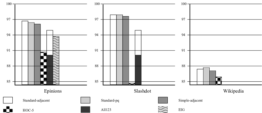
Figure 1: Prediction Accuracy of Different Peer Opinion Formulations, and Previous Results

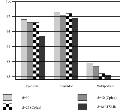
Figure 2: Prediction Accuracy for Different QUBO Solvers

As mentioned earlier, solving the quadratic optimization problem is an important and the most difficult part of our method. By decreasing the subset size $d$, we trade off the accuracy over efficiency. In the experiment, we assign different values to $d$ and measure the prediction accuracy. For $d=10$, we can solve the optimization problem exactly by brute-force. For $d>10$, we need to use Cplex-solver [1] to solve the problem. In Table 5 (see also Fig. 2), we compare the performance of our model with different values of $d$. We expect the prediction accuracy to increase as the value of $d$ increases. However, experimental result shows that it is not the case. As shown in the table, when $d=10$, our model gives a better prediction accuracy using exact solver instead of Cplex-solver. Since Cplex-solver only gives an approximate solution which effects the overall quality of the classifier, we do not see much improvements as $d$ increase. But still, we think the prediction accuracy should increase if we can a better solution for the problem for larger value of $d$. Indeed, when $d$ equal to the size of the original problem, we are solving the original problem directly instead of subdividing it into smaller problems. What seems to be the case is that the accuracy of the algorithm is very sensitive to the quality of approximation of the quadratic optimization problem.

We also include the results obtained by using the open source Max-SAT solver METSLib [2]. Although its approximation is clearly inferior to that of Cplex, it solves the entire problem whiout splitting it into small subproblems. So, the overall performance is similar to that of Cplex, except fo Epinion, for which the time limit set for Tabu search (1 sec) is apparently insufficient. Note as well that overall running time (although we did not make any precise measurements) using METSLib is considerably greater than that using Cplex.

Table 5: Prediction Accuracy of Different Values of $d$

Dataset	Epinions	Slashdot	Wikipedia
d=10 (exact)	96.36%	98.00%	87.69%
d=10 (cplex)	96.17%	97.31%	86.98%
d=25 (cplex)	96.20%	97.52%	85.60%
METSLib	93.03%	96.79%	86.22%

In [10] and [17] the authors use certain techniques to test their approaches on unbiased datasets. They use, however, different ways to balance the dataset and/or results. For instance, [10] do not change the dataset (Epinions), but, since the dataset is biased toward positive links, they find the error ratio separately for positive and negative links, and then average the results. More precisely, they test the method on a set of randomly sampled edges that naturally contains more positive edges. Then they record the error rate on all negative edges, sample randomly the same number of positive edges (from the test set), find the error rate on them, and report the mean of the two numbers.

The approach of [17] is different. Instead of balancing the results they balance the dataset itself. In order to do that they keep all the negative edges in the datasets, and then sample the same number of positive edges removing the rest of them. All the training and testing is done on the modified datasets. Although we have reservations about both approaches, we tested our model in these two settings as well. The results are shown in Table 6.

Table 6: Prediction Accuracy of Balanced Approach

Dataset	Epinions	Slashdot	Wikipedia
Standard-pd	85.14 %	82.82%	62.58%
(averaging the results)
of them false negative	0.84%	0.50%	2.10%
of them false positive	28.89%	33.8%	72.6%
Standard-pq	89.36%	86.37%	76.81%
(balancing the dataset)
of them false negative	6.20%	14.37%	22.5%
of them false positive	22.93%	15.35%	23.90%
All123 ([17])	93.42%	93.51%	80.21%
EIG ([10])	85.30%	N/A	N/A

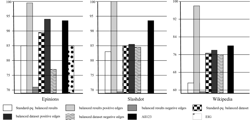
Figure 3: Prediction Accuracy of Balanced Approach. Negative Edges Bar for Slashdot and Wikipedia are out of Chart.

Observe that since our approach is to train the predictor for a particular dataset rather than finding and tuning up general features as it is done in [10] and [17], and the test datasets are biased toward positive edges, it is natural to expect that predictions are biased toward positive edges as well. This is clearly seen from Table 6 (see also Fig. 3). We therefore think that average error rate does not properly reflect the performance of our algorithm.

In the case of balanced datasets our predictor does not produce biased results, again as expected. This, however, is the only case when its performance is worse than some of the previous results. One way to explain this is to note that density of the dataset is crucial for accurate predictions made by the quadratic correlation approach. Therefore we had to lower the embeddedness threshold used in this part of the experiment to $p=5$, $q=5$, while [17] still tests only edges of embeddedness at least 25.

4.3 Recommender systems dataset

To test the versatility of the model, we also test it on a completely different dataset. MovieLens [3] is a dataset used primarily in the study of recommender systems. It contains rating of movies given by users who rented movies from a shop or online. Every user gives a rating to some of the movies by assigning a score from 1 to 5, where higher score corresponds to higher evaluation of the movie. It therefore can viewed as a bipartite graph with users in one part of the bipartition, and movies in the other. The version of the dataset we used, MovieLens-100k, contains approximately 100,000 ratings from 1000 users on 1700 movies. There are also certain density restriction: Every user included in the dataset must rate at least 20 movies.

It is natural to treat users ratings as attitudes of users towards movies. Our model, however, cannot work directly with the MovieLens dataset, because it requires binary attitudes rather ratings between 1 and 5. Thus, we convert user ratings into positive and negative attitudes, by introducing a negative link every time user’s rating is 3 or less, and by introducing a positive link if user’s rating is 4 or 5. Under such interpretation of scores the dataset is almost balanced, 44.625% of its edges are negative. Predictions are, of course, also made in terms of positive and negative links.

With the standard values of the parameters: using Standard-pq option with Cplex, and with $p=15$, $q=20$, $d=10$, the model makes about 75% correct predictions providing about 20% increase over the random guess. Although there is a very substantial amount of research on recommender systems using MovieLens as a test dataset (see e.g. [25, 24], it is not possible to compare our result against the existing ones, because the evaluation measures normally used for recommender systems are quite different; they measure either the success rate in recommending a group of products (movies) or given in terms of estimating user’s rating rather than attitude. Nevertheless we can conclude that the method gives a similar advantage over the random choice, as for other datasets. One interesting feature of the (internal) work of our method is that it finds influences and sets of trusted peers between users, although there is no explicit information about such connections.

5 Conclusion

We have investigated the link sign prediction problem in online social networks with a mixture of both positive and negative relationships. We have shown that a better prediction accuracy can be achieved using personalized features such as peer opinions. Moreover, the proposed model accommodates the dynamic nature of online social networks by building a predictor for each individual nodes independently. It enables fast updates as the underlaying network evolves over time.

In the future, we consider possible improvements of the model in two directions. First of all, we need to find a better formulation for peer opinions. The current formulation is very simple that it either gives an estimation or it doesn’t estimate. Ideally, we want a formulation that gives an estimation along with the confidence level of its estimation. The current choice of the binary representation of the problem was determined by several factors. Firstly, many more existing algorithms, heuristics, and off-the-shelf solvers are available for binary problems. This includes many readily available Max-SAT solvers. Some solvers, for example, Cplex, while can be used for non-binary problems, produce good results only if the problem satisfies certain conditions. We experimented with weights $w_{v,x}$ that can take more than just 2 values, but this often leads to instances that are not positive semidefinite, and Cplex does not produce any meaningful results. In spite of this we experimented by allowing various variables of the problem to take more values. However, it did not lead to any noticeable improvements of the results.

Secondly, we want to build a more sophisticated model that incorporates more information. The basic assumption of our model is that users’ actions can be determined by the opinions of their peers in the network. Yet, as an independent individual, we also have our own knowledge and belief. There are also external factors that affects our decision making process, such as mood, weather, location, and so on. All these information can be used as features for our model in the future.

References

- [1] IBM ILOG CPLEX Optimizer, http://www-01.ibm.com/software/integration/optimization/cplex-optimizer, 2010.
- [2] METSLib, https://projects.coin-or.org/metslib, 2011.
- [3] MovieLens Data Sets, http://www.grouplens.org/node/12, 2011.
- [4] Paolo Avesani, Paolo Massa, and Roberto Tiella, A trust-enhanced recommender system application: Moleskiing, SAC, 2005, pp. 1589–1593.
- [5] Michael J. Brzozowski, Tad Hogg, and Gábor Szabó, Friends and foes: ideological social networking, CHI, 2008, pp. 817–820.
- [6] Moira Burke and Robert Kraut, Mopping up: modeling wikipedia promotion decisions, CSCW, 2008, pp. 27–36.
- [7] Dorwin Cartwright and Frank Harary, Structure balance: A generalization of heider s theory, Psychological Review 63 (1956), no. 5, 277–293.
- [8] Kai-Yang Chiang, Nagarajan Natarajan, Ambuj Tewari, and Inderjit S. Dhillon, Exploiting longer cycles for link prediction in signed networks, CIKM, 2011, pp. 1157–1162.
- [9] Yoav Freund and Robert E. Schapire, A decision-theoretic generalization of on-line learning and an application to boosting, 1995.
- [10] Ramanathan V. Guha, Ravi Kumar, Prabhakar Raghavan, and Andrew Tomkins, Propagation of trust and distrust, WWW, 2004, pp. 403–412.
- [11] I. Guyon, S. Gunn, M. Nikravesh, and L.A. Zadeh, Feature extraction: foundations and applications, vol. 207, Springer, 2006.
- [12] Frank Harary, On the notion of balance of a signed graph, Michigan Math. Journal 2 (1953), no. 2, 143–146.
- [13] Mohammad Al Hasan, Vineet Chaoji, Saeed Salem, and Mohammed Zaki, Link prediction using supervised learning, In Proc. of SDM 06 workshop on Link Analysis, Counterterrorism and Security, 2006.
- [14] F. Heider, Attitudes and cognitive organization, J. Psych. 21 (1946), 107–112.
- [15] Jérôme Kunegis, Andreas Lommatzsch, and Christian Bauckhage, The slashdot zoo: mining a social network with negative edges, Proceedings of the 18th international conference on World wide web (New York, NY, USA), WWW ’09, ACM, 2009, pp. 741–750.
- [16] Cliff Lampe, Erik W. Johnston, and Paul Resnick, Follow the reader: filtering comments on slashdot, CHI, 2007, pp. 1253–1262.
- [17] Jure Leskovec, Daniel P. Huttenlocher, and Jon M. Kleinberg, Predicting positive and negative links in online social networks, WWW, 2010, pp. 641–650.
- [18] David Liben-Nowell and Jon Kleinberg, The link prediction problem for social networks, Proceedings of the twelfth international conference on Information and knowledge management (New York, NY, USA), CIKM ’03, ACM, 2003, pp. 556–559.
- [19] , The link-prediction problem for social networks, J. Am. Soc. Inf. Sci. Technol. 58 (2007), no. 7, 1019–1031.
- [20] et al. M. W. Johnson, Quantum annealing with manufactured spins, Nature 473 (2011), 194–198.
- [21] Paolo Massa and Paolo Avesani, Controversial users demand local trust metrics: An experimental study on epinions.com community, AAAI, 2005, pp. 121–126.
- [22] Hartmut Neven, Vasil S. Denchev, Geordie Rose, and William G. Macready, Training a large scale classifier with the quantum adiabatic algorithm, CoRR abs/0912.0779 (2009).
- [23] M.E.J. Newman, The structure and function of complex networks, SIAM Review 45 (2003), no. 2, 167–256.
- [24] John O’Donovan and Barry Smyth, Trust in recommender systems, IUI, 2005, pp. 167–174.
- [25] Badrul M. Sarwar, George Karypis, Joseph A. Konstan, and John Riedl, Analysis of recommendation algorithms for e-commerce, ACM Conference on Electronic Commerce, 2000, pp. 158–167.