Spectral description of the dynamics of ultracold interacting bosons in disordered lattices

Abstract

We study the dynamics of a nonlinear one-dimensional disordered system from a spectral point of view. The spectral entropy and the Lyapunov exponent are extracted from the short time dynamics, and shown to give a pertinent characterization of the different dynamical regimes. The chaotic and self-trapped regimes are governed by log-normal laws whose origin is traced to the exponential shape of the eigenstates of the linear problem. These quantities satisfy scaling laws depending on the initial state and explain the system behaviour at longer times.

1 Introduction

The motion of non-interacting particles in disordered lattices has been intensely studied over the last decades. In one and two dimensions, and for a sufficient amount of disorder in three dimensions, it has been shown that the spreading of quantum wavepackets is suppressed, a phenomenon known as Anderson localization [1, 2]. However, the celebrated Anderson model that leads to this prediction is a highly simplified model which in particular neglects particle-particle interactions, so that a crucial question is: Do interactions destroy (or, on the contrary, enhance) Anderson localization?

A burst of interest on the subject was recently driven by the demonstration that these questions could be studied experimentally and theoretically with an unprecedented degree of cleanness and precision using ultracold atoms. This has produced an impressive number of results, concerning both Anderson localization (AL) [3, 4, 5, 6, 7, 8] and the Anderson transition [9, 10, 11, 12], observed in 3D systems. Moreover, systems of ultracold bosons turned out to be very well modeled by mean-field approaches [13, 14], in contrast to fermionic systems where such a simplification of the corresponding many-body problem is not possible.

From the theoretical and numerical point of view, ultracold bosons in a 1D optical disordered lattice can be described rather realistically by a simple generalization of the original Anderson model including a nonlinear term taking into account interactions in a mean-field description. Numerical studies of the model suggest that the long term motion of the particles is subdiffusive [15, 16, 17, 18, 19, 20, 21]. These studies pointed out in particular the central role of chaotic dynamics in the destruction of AL.

This approach has however two important drawbacks. The first is that the timescale of subdiffusion is larger by several orders of magnitude than the timescale of the single-particle dynamics, implying very long computer calculations which make difficult a full study of the interplay between disorder and interactions. The second is that the nonlinearity leads to a strong dependence on the initial conditions which also makes it difficult to give a “global” characterization of the different dynamical regimes. In previous works, we have shown the existence of scaling laws with respect to the width of the initial state, allowing, to some extent, such a global characterization [21], and demonstrated that these scaling laws are robust with respect to decoherence effects  [22] (which can also destroy AL).

In the present work we tackle the problem of interacting ultracold bosons in a 1D disordered lattice using a spectral analysis that does not require such long computational times, as the information on the chaotic behaviour is “inscribed” even in early times in the spectrum of the dynamics. This allows us to perform a more complete and precise study of the problem over a large range of parameters. A central quantity in our study, the spectral entropy, proves very useful to characterize the dynamic behaviours, confirmed by comparing the information extracted from the spectral entropy to the Lyapunov exponent, another well-known measure of chaotic behaviour. Moreover, we show that such behaviours are described by “log-normal” laws which can be scaled with respect to the initial conditions, and we propose a simple physical interpretation of our findings.

2 The model

We use here the discrete nonlinear Schrödinger equation with diagonal disorder. It is essentially the same model used in previous works [21, 22], so we only give an outline of it here.

The mean-field theory applied to ultracold bosons in an optical (ordered) lattice leads to the so-called Gross-Pitaevskii equation:

$$i\hbar\dot{\phi}(x)=\left[\frac{p^{2}}{2m}+V(x)+g_{1D}N|\phi(x)|^{2}\right]\phi(x)$$

where $\phi$ is the macroscopic wavefunction (or order parameter) describing a Bose-Einstein condensate well below the critical temperature, $V(x)=-V_{0}\cos(2k_{L}x)$ is the optical potential and $g_{\mathrm{1D}}$ the 1D coupling constant [23]. Tight-binding equations are obtained by decomposing the wavefunction $\phi(x)=\sum_{n}c_{n}(t)w_{n}(x)$ onto the set of localized Wannier functions of the first band $w_{n}(x)$ associated to the $n^{\mathrm{th}}$ lattice site:

$$i\dot{c}_{n}=v_{n}c_{n}-c_{n-1}-c_{n+1}+g\left|c_{n}\right|^{2}c_{n},$$ (1)

where we kept only (symmetric) nearest-neighbours couplings, which is justified if the Wannier functions are strongly localized, that is, for large enough $V_{0}$. According to usual conventions, we measure distances in steps of the lattice and write energies in units of the coupling constant of neighbour sites $T=-\int dxw_{n}(x)[p^{2}/2m+V(x)]w_{n+1}(x)$ . Finally, times are written in units of $\hbar/T$. The coefficient $v_{n}=\int dxw_{n}(x)[p^{2}/2m+V(x)]w_{n}(x)/T$ is the diagonal on-site energy and the effect of interactions is taken into account, in a mean-field approach, by adding the nonlinear term $g\left|c_{n}\right|^{2}$ where the dimensionless interacting strength is

$$g=\frac{g_{\mathrm{1D}}N\int d_{x}|w_{0}|^{4}}{T}.$$

In the absence of disorder, the on-site energy $v_{n}$ does not depend on the site index $n$ and can be thus set to $0$. According to the Anderson’s postulate [1], we introduce diagonal disorder by picking random on-site energies $v_{n}$ uniformly in an interval $[-W/2,W/2]$.

For $g=0$, (1) describes the standard Anderson model, and we shall call the corresponding eigenstates (eigenvalues) “Anderson” eigenstates (eigenvalues). A few facts about it will be useful in what follows. The eigenstates are exponentially localized in average $\overline{c_{n}^{\nu}}\sim\exp\left(-|n|/l_{\nu}\right)$ (the overbar indicates the averaging over realizations of the disorder) with a localization length $l_{\nu}(W)\sim 96(1-\epsilon_{\nu}^{2}/4)/W^{2}$ [24]. For $g\neq 0$ the equation becomes nonlinear, and it is useful, if not strictly rigorous, to interpret the nonlinear term as a “dynamical correction” to the on-site energy $v_{n}^{\mathrm{NL}}=g|c_{n}|^{2}$. Previous works [15, 16, 17, 20, 18, 21] put into evidence the existence of three main dynamical regimes: For $g\ll W$, Anderson localization is expected to survive for very long times, a regime that we shall call “quasi-localized”. For $g\sim W$, the nonlinear correction $v_{n}^{\mathrm{NL}}$ induces chaotic dynamics leading to subdiffusion and the destruction of AL. For $g\gg W$, the very large nonlinear term $v_{n}^{\mathrm{NL}}$ decouples all sites whose populations are not nearly equal (even in the absence of the disorder), suppressing the diffusive behaviour and leading to another type of localization, called self-trapping. This dynamics does not rely on quantum interference and is therefore very robust against external perturbations, including decoherence [22].

Our aim is to characterize the global dynamics on a relatively short timescale. We thus study the evolution according to (1) of bosons in a 1D box containing $L$ sites (typically, $L=101$) and put an exponential absorber at each end of the box in order to prevent wavepacket reflection. The norm of the wavepacket is thus not anymore conserved as soon as it “touches” the borders, and we characterize the diffusive behaviour by calculating the survival probability $p(t)=\sum_{n}|c_{n}|^{2}$; a value $p(t)<1$ indicates that the packet has diffused outside the box. As in ref. [21], we restrict the analysis to initial wavepackets of the form

$$c_{n}(t=0)=\cases{L_{0}^{-1/2}\exp\left(i\theta_{n}\right)&$|n|\leq\left(L_{0}-1\right)/2$\\ 0&overwise}$$

with $L_{0}\ll L$ .

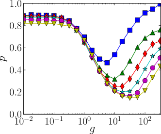
Figure 1: Survival probability $p$ at time $t=10^{5}$ vs interaction strength $g$ for $W=4$ and different widths of the initial state : $L_{0}=$3 (blue squares), 7 (green triangles), 13 (red diamonds), 21 (cyan stars), 31 (magenta circles), 41 (yellow inverted triangles).

The typical behaviour of the survival probability is illustrated in figure 1, which represents $p(g,t=10^{5})$ as a function of the interaction strength $g$ for $W=4$ and for various values of $L_{0}$. To obtain such smooth curves, the survival probability was averaged over typically $500$ realizations of the disorder and of the initial phases $\theta_{n}$. Such long times are necessary in order to clearly put into evidence the three different regimes mentioned above, which are then easily identifiable: At low $g$, the survival probability is close to one, corresponding to the quasi-localized regime in which AL survives. For intermediate values of $g$, the decrease of $p$ indicates that the wave packet has spread along the box and part of it has been absorbed at the borders, corresponding to a chaotic regime induced by the nonlinearity that destroys AL. For large values of $g$, the survival probability increases again and gets close to $1$, indicating that the packet is self-trapped [15, 16, 21] and has never touched the borders if initially it was thin enough (e.g. in the $L_{0}=3$ case). In the next section, we show that a complementary way to describe the dynamics allows to a very precise characterization within much shorter computation times.

3 Characterizing chaotic dynamics with the spectral entropy

Spectral analysis is a very useful way of analyzing a chaotic dynamics, be it in classical, “quantum” or quantum nonlinear chaotic systems [25]. The spectral entropy is a measure of the “richness” of a spectrum. Chaotic behaviours are associated to continuous spectra, and thus to a high spectral entropy. Given a quantity $M(t)$, its power spectrum is defined as

$$S_{f}[M(t)]=\frac{\left|\tilde{M}(f)\right|^{2}}{\int_{0}^{f_{\max}}df\left|\tilde{M}(f)\right|^{2}}\quad,f\in[0,f_{\max}]$$

where $\tilde{M}(f)$ is the Fourier transform of $M(t)$ for $t\in[0,t_{\max}]$. The choice of the value of $t_{\max}$ determines the resolution of the spectrum. In our case, we chose $t_{\max}=200$, which is a very small value compared to the typical time of emergence of the interacting regime ($t\sim 10^{5}$) but which will be shown to be sufficiently high to characterize the dynamics from a spectral point a view. As we do not expect excitations whose timescale is inferior to the tunneling time ($1$ in our rescaled units), we set $f_{\mathrm{max}}=1$ . From the power spectrum, one defines the spectral entropy as

$$H=-\frac{\int df\ S(f)\log S(f)}{\log(f_{\mathrm{max}})}.$$ (2)

For a perfectly monochromatic signal $S_{f}=\delta(f-f_{0})$, the spectral entropy is zero, whereas for a white noise ($S_{f}=1/f_{\mathrm{max}}$) $H=1$. The spectral entropy “counts” the number of frequencies which are present in the signal, and is a good indicator of the chaoticity of the system [26]. The spectral entropy obviously strongly depends on the choice of the observable, and its usefulness as a dynamics indicator is reliant on this choice.

A good observable in the present problem is the so-called “participation number” $P$ with respect to the Anderson eigenstates, which is defined, in the present case, as follows. For a given realization of disorder $\{v_{n}\}$, we calculate the Anderson eigenstates in the Wannier basis, $\phi_{\nu}(x)=\sum_{n}d_{n}^{(\nu)}w_{n}(x)$ corresponding to an energy $\epsilon_{\nu}$, which are solutions of (1) with $g=0$ (the $d_{n}^{(\nu)}$ replacing the $c_{n}$). Back to the $g\neq 0$ case, Equation (1) allows us to calculate the evolution of the wavepacket $\psi(t)=\sum c_{n}(t)w_{n}(x)$ under the action of both disorder and nonlinearity. At any time, we can express the wavepacket in the Anderson eigenstates basis

$$\psi(t)=\sum_{\nu}q_{\nu}(t)\phi_{\nu}(x),$$ (3)

from which, trivially, $q_{\nu}(t)=\sum_{n}d_{n}^{(\nu)}c_{n}(t)$. The participation number is then defined as:

$$P=\frac{\sum_{\nu}|q_{\nu}|^{2}}{\sum_{\nu}|q_{\nu}|^{4}}.$$ (4)

If $g=0$, the $\phi_{\nu}$ are the exact eigenstates of the problem, so that the populations $|q_{\nu}|^{2}$ are constant. In the non-interacting case $g\neq\text{0}$, the $|q_{\nu}|^{2}$ evolve under the action of the nonlinearity. The participation number roughly “counts” the number of Anderson eigenstates participating significantly in the dynamics and its time evolution thus reflects the apparition of Anderson eigenstates that were not initially populated.

Figure 2 shows the spectral power $S(f)$ of the participation number $P$ in the three interacting regimes: (a) $g=1$ in the quasi-localized regime, (b) $g=100$ in the chaotic regime, and (c) $g=1000$ in the self-trapping regime. For $g=1$, the dynamics is very similar to the linear case: The populations of Anderson eigenstates practically do not evolve in time, as well as the participation number $P$ and the spectrum is dominated by low frequencies. As a consequence, the spectral entropy, calculated according to (2), is relatively small: $H=10^{-2}$. For $g=100$, Anderson eigenstates are strongly coupled by the nonlinear term, each pair of coupled states generating a Bohr frequency (shifted by the nonlinear correction), that is $\sim\epsilon_{\nu}+g\left|q_{\nu}\right|^{2}-\epsilon_{\nu^{\prime}}-g\left|q_{\nu^{\prime}}\right|^{2}$. In this regime, most Anderson eigenstates are coupled to each other, so that the power spectrum is almost flat (with important local fluctuations) at high frequencies, and the spectral entropy increases by almost an order of magnitude $H=10^{-1}$ with respect to the preceding case. For $g=1000$ the wavepacket is self-trapped and only a relatively small number of Anderson eigenstates whose populations happen to be close enough can interact. The spectrum is therefore dominated by a finite number of frequencies and the spectral entropy is reduced, $H=2\times 10^{-2}$. However, although populations are stable in this case, quantum phases may evolve chaotically under the action of the nonlinearity [27]. Our definition of the spectral entropy from the participation number – which does not directly depends on the phases – excludes this “phase dynamics” from the corresponding spectrum.

      

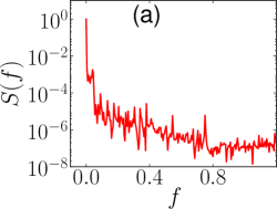
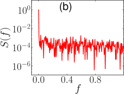
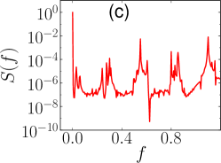
Figure 2: Example of spectral power $S(f)$ for the three different regimes : a) localized $g=1$, b) chaotic $g=100$ and c) self-trapped $g=1000$ . Other parameters are $W=3$, $L_{0}=3$ and $t_{\max}=200$.

We display in figure 3a the averaged spectral entropy as a function of the nonlinearity parameter $g$ for different widths $L_{0}$ of the initial state. One clearly sees the crossover from the quasi-localized to the chaotic regime, signalled by a marked increase of $H$. The smaller the value of $L_{0}$, the smaller the value of the crossover. This is easily understandable, as a more concentrated wavepacket leads to a stronger nonlinear term $v^{\mathrm{NL}}$. On the right side of the plot, one also sees, especially for low values of $L_{0}$ the beginning of a decrease of $H$ due to self-trapping.

It is interesting to compare the information obtained from the spectral entropy to another relevant quantity characterizing chaos, the Lyapunov exponent, which indicates how exponentially fast neighbour trajectories diverge. This quantity is usually defined for classical systems, but can be extended, with a little care, for quantum nonlinear systems [25]. We present in A a method for calculating the Lyapunov exponent of a quantum trajectory defined by amplitudes $c_{n}$ [Equation (1)]. Figure 3b displays the Lyapunov exponent $\lambda$ obtained with the same parameters as in figure 3a. It displays a monotonous increase with the nonlinear parameter, even in the region where the spectral entropy decreases due to self-trapping, evidencing the presence of a regime of “phase chaos” mentioned above. This clearly shows that $H$ and $\lambda$ provide different information on the dynamics of the system, and that $H$ is clearly more adapted to distinguish the three dynamical regimes.

In section 4 we will discuss the shape of these curves, their scaling properties, and suggest a physical mechanism explaining such properties.

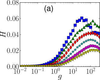
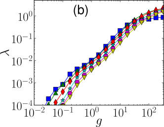
Figure 3: (a) Spectral entropy $H$ and (b) Lyapunov exponent $\lambda$ vs interaction strength $g$ for $W=4$ and different widths of the initial state : $L_{0}=$3 (blue squares), 7 (green triangles), 13 (red diamonds), 21 (cyan stars), 31 (magenta circles), 41 (yellow inverted triangles).

4 Log-normal law and scaling

As we shall see below, log-normal functions are ubiquitous in the dynamics described in the present work, and so in various contexts which are not obviously related to each other. A first example can be found in figure 1, where each curve representing $p(\log g)$ can be fitted with a rather good accuracy by a inverted Gaussian function. More generally, a log-normal function is defined as

$$f(x) = \frac{1}{x}\exp\left[-\frac{\left(\log x-\mu\right)^{2}}{2\sigma^{2}}\right]$$

$$= \exp(-\mu+\frac{\sigma^{2}}{2})\exp\left[-\frac{(\log x-\mu+\sigma^{2})^{2}}{2\sigma^{2}}\right]$$

In physics, such a function appears more often as a “log-normal distribution”, related to the statistics of quantities which are a product of randomly distributed terms [28]. Log-normal statistics is very different from normal (Gaussian) statistics; for example, the most probable value of a log-normally distributed quantity is different from its average value. In the following, we shall not only consider statistical distributions over the realizations of the disorder: figure 1 does not display the distribution of $p$ over the realizations of disorder but its average as a function of the interacting strength, so does figure 3a for the spectral entropy. However and more interestingly, we now show that the statistical distribution of the spectral entropy and of the Lyapunov exponent are indeed log-normal.

Let us thus study the distribution of these two quantities over the realizations of the disorder $v_{n}$ and of the initial phases $\theta_{n}$. Figure 4a displays the distributions of values of $H$ over $10^{4}$ realizations of the disorder for two values of $g$, and figure 4b the corresponding distribution for the Lyapunov exponent $\lambda$. As shown by the black fitting lines, both curves are perfectly fitted by a log-normal function.

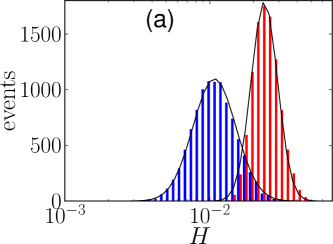
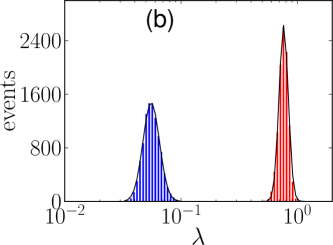
Figure 4: Histograms of the spectral entropy $H$ (a) and the Lyapunov exponent $\lambda$ (b) for $W=3$, $L_{0}=41$ and two interacting strengths : $g=10$ (left hand-side blue histogram), $g=100$ (right hand-side red histogram). Black solid lines correspond to log-normal fits.

In order to have an idea of the origin of these shapes, one can consider a simple, heuristic model. The destruction of AL is due to the nonlinear coupling between Anderson eigenstates. Initially unpopulated eigenstates, which, in the absence of nonlinearity, would never be populated, can be thus excited thanks to a nonlinear transfer of population. The goal of the simple model developed below is to characterize the statistical distribution of such excitations. Projecting the wavepacket in the Anderson eigenbasis [cf. Equation (3)], (1) then reads:

$$i\dot{q}_{\nu}=\epsilon_{\nu}q_{\nu}+g\sum_{\nu_{1},\nu_{2},\nu_{3}}q_{\nu_{1}}^{*}q_{\nu_{2}}q_{\nu_{3}}I(\nu,\nu_{1},\nu_{2},\nu_{3})$$ (5)

with $I(\nu,\nu_{1},\nu_{2},\nu_{3})=\sum_{n}d_{n}^{(\nu)}d_{n}^{(\nu_{1})}d_{n}^{(\nu_{2})}d_{n}^{(\nu_{3})}$. Populations exchanges are controlled by the overlap $I$ of four coefficients. The population transfer from eigenstate $\mu$ to eigenstate $\nu$ depends on $J_{1}=I(\mu,\mu,\nu,\nu)$, $J_{2}=I(\mu,\mu,\mu,\nu)$ and $J_{3}=I(\mu,\nu,\nu,\nu)$ , the term due to $J_{1}$ being for instance :

$$\frac{d\left|q_{\nu}\right|^{2}}{dt}=2gJ_{1}\,\mathrm{Im}\left(q_{\nu}^{*2}q_{\mu}^{2}\right)$$

In order to evaluate the probability distribution of $J_{1}$, we make the assumption that the coupled Anderson eigenstates are exponentially localized with the same localization length $\xi$. The exponential localization is valid on the average and the localization length is the same if the eigenstates have close enough eigenenergies. We thus write

$$d_{n}^{(\nu)}{}^{2} = \tanh\left(\frac{1}{\xi}\right)\exp\left(-\frac{2|n|}{\xi}\right)$$

$$d_{n}^{(\mu)}{}^{2} = \tanh\left(\frac{1}{\xi}\right)\exp\left(-\frac{2|n-l(\mu,\nu)|}{\xi}\right).$$

The overlap sum $J_{1}$ can then be written as

$$J_{1}=\tanh^{2}\left(\frac{1}{\xi}\right)e^{-2l(\mu,\nu)\text{/$\xi$}}\left[\frac{2}{1-e^{-4/\xi}}+l(\mu,\nu)-1\right]$$ (6)

where, for simplicity, we have supposed that the spatial distance between the eigenstates, $l(\mu,\nu)$, is an integer. The most important term in (6) is $e^{-2l(\mu,\nu)/\xi}$. In the limit $\xi\to 0$:

$$J_{1}=e^{-2l(\mu,\nu)/\xi}\left[l(\mu,\nu)+1\right]$$

The inverse localization length $\Lambda=1/\xi$ follows a normal distribution [29, 24]

$$P(\Lambda)\propto\exp[-(\Lambda-\Lambda_{0})^{2}/2\sigma^{2}]$$

we obtain for the distribution of values of the overlap $J_{1}$

$$P(J_{1}) = P(\Lambda)\left|\frac{d\Lambda}{dJ_{1}}\right|$$

$$\propto \frac{1}{J_{1}}\exp\left[-\frac{(\Lambda-\Lambda_{0})^{2}}{2\sigma^{2}}\right]$$

$$\propto \frac{1}{J_{1}}\exp\left[-\frac{\left(\log J_{1}-G\right)^{2}}{2\tilde{\sigma}^{2}}\right]$$

where $G=\log\left[l(\mu,\nu)+1\right]-2l(\mu,\nu)\Lambda_{0}$ and $\tilde{\sigma}^{2}=4l(\mu,\nu)^{2}\sigma^{2}$. The overlap sum $J_{1}$ thus obeys a log-normal distribution.

We conjecture that overlap sums like $J_{1}$, controlling the coupling between Anderson eigenstates, in fact control the destruction of the Anderson localization, and thus explain the log-normal shapes we observed for $H$ and $\lambda$. The above heuristic argument undoubtedly presents various assumptions that are not rigorously justified, but it has the merit of putting into evidence the intimate relation between the log-normal distribution and the exponential localization of the Anderson eigenstates. The link between the exponential shape and the emergence of log-normal statistics has also been studied in the case of the conductance of disordered systems [30, 31, 24].

Let us now consider the averaged spectral entropy. In previous works [21, 22], we showed that suitable scaling with respect to the initial state width $L_{0}$ allowed a classification of dynamic regimes independently of the shape of the initial state. In particular the interacting strength $g$ was scaled as $\tilde{g}=gL_{0}^{-s}$ with $s\approx 3/4$. This scaling is meaningless for low values of $L_{0}$ because in this case, the initial participation number is not of the order of $L_{0}$ but is of the order of the maximum Anderson localization length $\ell_{0}(W)\sim 96/W^{2}$. Figure 5a shows that scaling with $\tilde{g}$ and $\tilde{H}=HL_{0}^{s}$ make the curves $H(g)$ corresponding to $L_{0}\gtrsim 20$ collapse to a single curve, except in the strong self-trapped region. Figure 5b shows the Lyapunov exponent as a function of $\tilde{g}$; the curves also collapse for $L_{0}\gtrsim 12$. The Lyapunov exponent itself is independent of $L_{0}$ (with no scaling of the variable $\lambda$), which is not surprising as it does not measure the absolute distance between two quantum trajectories but the timescale of their exponential divergence.

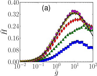
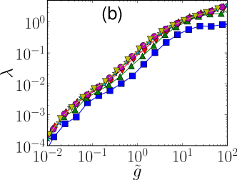
Figure 5: (a) rescaled spectral entropy $\tilde{H}=HL_{0}^{s}$ with $s\approx 3/4$ and (b) Lyapunov exponent $\lambda$ vs the rescaled interaction strength $\tilde{g}$ for $W=4$ and for $L_{0}=$3 (blue squares), 7 (green triangles), 13 (red diamonds), 21 (cyan stars), 31 (magenta circles), 41 (yellow inverted triangles).

As shown by the black solid line in figure 5a, the scaled spectral entropy $\tilde{H}$ is very well fitted (outside the strong self-trapped region $\tilde{g}>100$) by the log-normal law:

$$\tilde{H}=\frac{h_{0}}{\tilde{g}\sqrt{2\pi\sigma^{2}}}\exp\left[-\frac{(\log\tilde{g}-G)^{2}}{2\sigma^{2}}\right]$$ (7)

with three free parameters, the amplitude $h_{0}$, the center $G$ of the distribution and the “standard deviation” $\sigma$. The study of these fitting parameters as a function of the disorder $W$ provides a full characterization of the dynamic regime. Instead of representing the fit parameters $h_{0}$ and $G$, we prefer to use more physical quantities, namely the maximum value of $\tilde{H}$, $\tilde{H}_{\max}=\left[h_{0}\left(2\pi\sigma^{2}\right)^{-1/2}\right]\exp\left(\sigma^{2}/2-G\right)$ (figure 6a) and the rescaled interaction strength $\tilde{g}_{c}=\exp\left(G-\sigma^{2}\right)$ (figure 6b) corresponding to this maximum. The dependence of the standard deviation $\sigma$ on $W$ is displayed in figure 6c. The quantity $\tilde{H}_{\max}$ is a decreasing function of $W$: as the localization length decreases with $W$, so does the overlap between two neighbour Anderson eigenstates. On the contrary, $\tilde{g}_{\mathrm{c}}$ is an increasing function of $W$: The number of resonances is maximum when $v_{n}^{\mathrm{NL}}$ is comparable to the typical energy between two neighbour states, itself of the order of the bandwidth $\sim 4+W$; $\tilde{g}_{\mathrm{c}}$ is thus independent of $W$ at low disorders and increases with $W$ for larger disorders. Finally, in figure 6c, one can notice that the log-normal curve becomes sharper when the disorder increases, which can be attributed to the fact that Anderson Localization is more robust against interactions at high disorders.

      

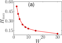
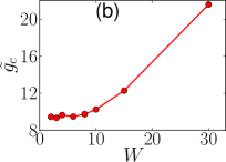
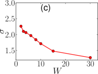
Figure 6: a) Maximum entropy $\tilde{H}_{\max}$, b) corresponding interaction strength $\tilde{g}_{\mathrm{c}}$ and c) resonant width $\sigma$ vs disorder $W$.

The fact that the spectral entropy can be determined from a relatively short time interval also allows one to follow the evolution of the dynamics. Figure 7 shows the evolution of the spectral entropy $H(t)$, defined as the spectral entropy calculated in an interval $[t,t+200]$ , that we shall call, for short, the dynamic spectral entropy. For the low value of $g=10$ (figure 7a), after the destruction of AL, the diffusion of the wavepacket produces a dilution and a consequent diminution of the nonlinearity that reduces the chaoticity, and thus the spectral entropy of the system. For the high value of $g=1000$ (figure 7b) one sees a more complex interplay of different regimes: The initial state is initially frozen in a self-trapping regime, but this regime is unstable (for this particular set of parameters): If a fraction of the packet escapes the self-trapped region, the nonlinear contribution $v_{n}^{\mathrm{NL}}$ decreases which leads to a weakening of the trapping. The destruction of the self-trapping regime takes a much longer time that the destruction of the AL. One first observes a small decrease of the spectral entropy, as some eigenstates leave the box and do not interact anymore. Then, when $v_{n}^{\mathrm{NL}}$ has decreased sufficiently in the center of the packet, the system enters the chaotic regime.

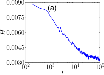
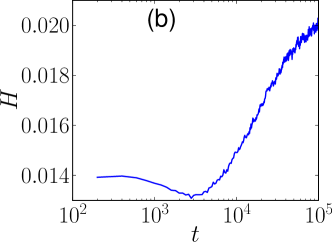
Figure 7: Evolution of the spectral entropy $H(t)$ for $W=4,$ $L_{0}=41$. For (a) $g=10$ one essentially sees the effect of dilution, which progressively weakens the chaoticity of the system. For (b) $g=10^{3}$, there is a first phase, in which the self-trapping is progressively destroyed which is followed by a slow transition towards the chaotic regime.

In plots a and b of figure 8 we represented the dynamic spectral entropy $H(t)$ for three values of $L_{0}$, corresponding to a same value of $\tilde{g}$ (0.62 in a, 6.17 in b and c). The curves converge for long times, putting into evidence the existence of a universal asymptotic regime, independent of the initial state, once the proper scaling on $\tilde{g}$ is applied. Additional scaling can even be used to describe the transition from the self-trapping regime to the chaotic regime, as shown in figure 8c. Although we have presently no physical explanation for the exponents appearing in these scaling laws, these results strongly support the idea that the features of the nonlinear dynamics should be scaled again with respect to the initial state [21].

      

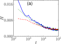
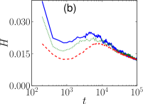
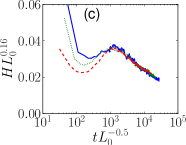
Figure 8: Scaling of the spectral entropy $H(t)$ for $W=4$ and $L_{0}=13$ (blue full line), $L_{0}=21$ (green dotted) and $L_{0}=41$ (red dashed). The use of the same values of the scaled nonlinearity $\tilde{g}=gL_{0}^{-s}$ [$\tilde{g}=0.62$ (a) and $\tilde{g}=6.17$ (b)] shows that there is a universal asymptotic regime. Comparison of plots (b) and (c) shows that additional adhoc scaling gives an even more universal character to this behaviour.

5 Conclusion

We have shown that the spectral entropy is a very good indicator of the chaoticity of the dynamics, and allows a very good characterization of the dynamics regimes. Moreover, it can be calculated dynamically and also gives information on the evolution of the dynamics. The Lyapunov exponent gives, in the present context, a less complete characterization of the dynamics. It describes very well the progressive destruction of the Anderson Localization by the onset of chaotic behaviour, exactly as the spectral entropy, but it does not give information in the self trapping regime, where “phase chaos” is still present.

The argument presented in section 4 suggests that the log-normal shape is linked to the exponential localization of the Anderson eigenstates. It is a bit surprising to find this link between the behaviour of a strongly nonlinear system and the eigenstates of the corresponding linear system. From a mathematical viewpoint, spectral analysis (in the sense of the determination of eigenvalues and eigenvectors) cannot be directly applied to nonlinear systems, and, presently, there is no alternative analytical method for analyzing nonlinear systems. The results discussed in the present work and in refs. [21, 22] indicate that scaling over the initial state is a promising tool for the study of the emerging field of nonlinear quantum mechanics. In this context, it is worth noting that we have presently no convincing explanation for the precise values of the exponents appearing in these scaling laws, and that we have considered only a particularly simple family of initial states. Moreover, there is no experimental verification of these scaling laws. It thus appears that a large field of investigations is opened for both theoreticians and experimentalists in the near future.

Appendix A Lyapunov exponent of a quantum trajectory

We are interested in calculating the Lyapunov exponent of the quantum trajectory $c\equiv(c_{n})$. Considering two initial conditions $c^{a}$, $c^{b}$, which are separated by an infinitesimal distance $d_{0}$, the Lyapunov exponent measures the rate of their exponential divergence.

$$\lambda=\lim_{t\to\infty}\frac{1}{t}\log\frac{d(t)}{d_{0}}$$ (8)

where $d(t)=|c^{b}(t)-c^{a}(t)|$. In principle, one could use directly (8) but it turns out that the trajectories do not evolve in an ensemble of infinite volume. As a consequence the distance $d(t)$ rapidly saturates and $\lambda$ tends to $0$. The common method to get rid of this drawback is to let trajectories evolve during a short time period $d_{t}$ and then evaluate the corresponding Lyapunov exponent

$$\lambda_{0}=\frac{1}{d_{t}}\log\frac{d_{1}}{d_{0}}$$ (9)

where $d_{1}=|c^{b}(d_{t})-c^{a}(d_{t})|$. Before letting the system evolve for another time interval $d_{t}$, we rescale trajectories so that the distance between $a$ and $b$ is set to $d_{0}$ keeping their relative orientation unchanged. Usually, people rescale the second trajectory $\tilde{c}^{b}=c^{b}+\frac{d_{0}}{d_{1}}(c^{b}-c^{a})$ satisfying immediately both requirements. We then obtain $\lambda_{1},\lambda_{2},..$ by iterating the three-steps operation : (i) evolution during a short time $d_{t}$ (ii) calculation of the corresponding Lyapunov exponent from (9) (iii) renormalization of the trajectories. We finally deduce the final Lyapunov exponent :

$$\lambda=\lim_{N\to\infty}\frac{1}{N}\sum_{i=1}^{N}\lambda_{i}$$

where $N$ represents the number of iterations. Unfortunately, the crucial rescaling operation changes the norm of the second trajectory $c_{b}$ : in the case of quantum systems, the procedure is therefore based on non-physical states. Here we propose to modify the step (iii) rescaling both trajectories using the following scheme :

$$\tilde{c}^{a} = \alpha c^{a}+\beta c^{b}$$

$$\tilde{c}^{b} = \gamma c^{a}+\delta c^{b}$$

where $(\alpha,\beta,\gamma,\delta)$ satisfy the following conditions :

$$\tilde{c}^{b}-\tilde{c}^{a} = \frac{d_{0}}{d_{1}}\left(c^{b}-c^{a}\right)$$ (10)

$$|\tilde{c}^{a}|^{2} = 1$$ (11)

$$|\tilde{c}^{b}|^{2} = 1$$ (12)

Given that $d_{1}=|c^{b}-c^{a}|$, the first equation is nothing but the usual scaling condition which is used for classical systems. Projecting (10) on $c^{a}$ and on $c^{b}$, one immediately obtains

$$\gamma = \alpha-\frac{d_{0}}{d_{1}}$$

$$\delta = \beta+\frac{d_{0}}{d_{1}}$$

Subtracting (11) from (12), and using $2\Re\langle c^{a}|c^{b}\rangle=2-d_{1}^{2}$, we obtain

$$\beta=\alpha-\frac{d_{0}}{d_{1}}$$

and finally from (11), we can choose

$$\alpha=\frac{d_{0}}{2d_{1}}+\frac{1}{2}\sqrt{\frac{4-d_{0}^{2}}{4-d_{1}^{2}}}$$

to finally deduce $\beta,\gamma,\delta$. This method allows an accurate calculation of the Lyapunov exponent in the discrete system considered in the present work, but it can in principle be also applied to the continuous Gross-Pitaevskii equation.

References

References

- [1] P. W. Anderson. Absence of Diffusion in Certain Random Lattices. Phys. Rev., 109(5):1492–1505, 1958.
- [2] E. Abrahams, P. W. Anderson, D. C. Licciardello, and T. V. Ramakrishnan. Scaling Theory of Localization: Absence of Quantum Diffusion in Two Dimensions. Phys. Rev. Lett., 42(10):673–676, 1979.
- [3] F. L. Moore, J. C. Robinson, C. F. Bharucha, B. Sundaram, and M. G. Raizen. Atom Optics Realization of the Quantum -Kicked Rotor. Phys. Rev. Lett., 75(25):4598–4601, 1995.
- [4] J. Billy, V. Josse, Z. Zuo, A. Bernard, B. Hambrecht, P. Lugan, D. Clément, L. Sanchez-Palencia, P. Bouyer, and A. Aspect. Direct observation of Anderson localization of matter-waves in a controlled disorder. Nature (London), 453:891–894, 2008.
- [5] G. Roati, C. d’Errico, L. Fallani, M. Fattori, C. Fort, M. Zaccanti, G. Modugno, M. Modugno, and M. Inguscio. Anderson localization of a non-interacting Bose-Einstein condensate. Nature (London), 453:895–898, 2008.
- [6] S. S. Kondov, W. R. McGehee, J. J. Zirbel, and B. DeMarco. Three-Dimensional Anderson Localization of Ultracold Matter. Science, 334(6052):66 –68, 2011.
- [7] F. Jendrzejewski, A. Bernard, K. Muller, P. Cheinet, V. Josse, M. Piraud, L. Pezze, L. Sanchez-Palencia, A. Aspect, and P. Bouyer. Three-dimensional localization of ultracold atoms in an optical disordered potential. Nat. Phys., 8(5):398–403, 2012.
- [8] H. Lignier, J. Chabé, D. Delande, J. C. Garreau, and P. Szriftgiser. Reversible Destruction of Dynamical Localization. Phys. Rev. Lett., 95(23):234101, 2005.
- [9] J. Chabé, G. Lemarié, B. Grémaud, D. Delande, P. Szriftgiser, and J. C. Garreau. Experimental Observation of the Anderson Metal-Insulator Transition with Atomic Matter Waves. Phys. Rev. Lett., 101(25):255702, 2008.
- [10] G. Lemarié, J. Chabé, P. Szriftgiser, J. C. Garreau, B. Grémaud, and D. Delande. Observation of the Anderson metal-insulator transition with atomic matter waves: Theory and experiment. Phys. Rev. A, 80(4):043626, 2009.
- [11] G. Lemarié, H. Lignier, D. Delande, P. Szriftgiser, and J. C. Garreau. Critical State of the Anderson Transition: Between a Metal and an Insulator. Phys. Rev. Lett., 105(9):090601, 2010.
- [12] M. Lopez, J.-F. Clément, P. Szriftgiser, J. C. Garreau, and D. Delande. Experimental Test of Universality of the Anderson Transition. Phys. Rev. Lett., 108(9):095701, 2012.
- [13] F. Dalfovo, S. Giorgini, L. Pitaevskii, and S. Stringari. Theory of Bose-Einstein condensation in trapped gases. Rev. Mod. Phys., 71:463–512, 1999.
- [14] I. Bloch, J. Dalibard, and W. Zwerger. Many-body physics with ultracold gases. Rev. Mod. Phys., 80(3):885–964, 2008.
- [15] A. S. Pikovsky and D. L. Shepelyansky. Destruction of Anderson Localization by a Weak Nonlinearity. Phys. Rev. Lett., 100(9):094101, 2008.
- [16] S. Flach, D. O. Krimer, and C. Skokos. Universal Spreading of Wave Packets in Disordered Nonlinear Systems. Phys. Rev. Lett., 102(2):024101, 2009.
- [17] T V Laptyeva, J D Bodyfelt, D O Krimer, C Skokos, and S Flach. The crossover from strong to weak chaos for nonlinear waves in disordered systems. Europhys. Lett., 91(3):30001, 2010.
- [18] A. Pikovsky and S. Fishman. Scaling properties of weak chaos in nonlinear disordered lattices. Phys. Rev. E, 83(2):025201(R), 2011.
- [19] D.M. Basko. Weak chaos in the disordered nonlinear Schrödinger chain: Destruction of Anderson localization by Arnold diffusion. Annals of Physics, 326(7):1577–1655, July 2011.
- [20] M. Ivanchenko, T. Laptyeva, and S. Flach. Anderson Localization or Nonlinear Waves: A Matter of Probability. Physical Review Letters, 107(24):240602–, December 2011.
- [21] B. Vermersch and J. C. Garreau. Interacting ultracold bosons in disordered lattices: Sensitivity of the dynamics to the initial state. Phys. Rev. E, 85(4):046213, 2012.
- [22] B. Vermersch and J. C. Garreau. Decoherence effects in the dynamics of interacting ultracold bosons in disordered lattices. arXiv:1209.4550, September 2012.
- [23] D. S. Petrov, D. M. Gangardt, and G. V. Shlyapnikov. Low-dimensional trapped gases. J. Phys. IV (France), 116:5–44, 2004.
- [24] C. A. Mueller and D. Delande. Disorder and interference: localization phenomena. 2010.
- [25] M. Lepers, V. Zehnlé, and J. C. Garreau. Tracking Quasiclassical Chaos in Ultracold Boson Gases. Phys. Rev. Lett., 101(14):144103, 2008.
- [26] I. A. Rezek and S. J. Roberts. Stochastic complexity measures for physiological signal analysis. IEEE Trans. Biomed. Eng., 45(9):1186–1191, 1998.
- [27] Q. Thommen, J. C. Garreau, and V. Zehnlé. Classical Chaos with Bose-Einstein Condensates in Tilted Optical Lattices. Phys. Rev. Lett., 91(21):210405, 2003.
- [28] E. Limpert, W. A. Stahel, and M. Abbt. Log-normal distibutions across the sciences: Keys and Clues. BioScience, 51(5):341–352, 2001.
- [29] O. A. Starykh, P. R. J. Jacquod, E. E. Narimanov, and A. D. Stone. Signature of dynamical localization in the resonance width distribution of wave-chaotic dielectric cavities. Phys. Rev. E, 62(2):2078–2084, 2000.
- [30] S. A. van Langen, P. W. Brouwer, and C. W. J. Beenakker. Nonperturbative calculation of the probability distribution of plane-wave transmission through a disordered waveguide. Phys. Rev. E, 53(2):R1344–R1347, 1996.
- [31] F. Evers and A. D. Mirlin. Anderson transitions. Rev. Mod. Phys., 80(4):1355–1417, 2008.